rng = np.random.default_rng()
x = np.concatenate([rng.normal(-2.0, 0.8, 300), rng.normal(1.5, 0.6, 200)])

def gauss(x, mu, sigma):
    return np.exp(-0.5 * ((x - mu) / sigma)**2) / (sigma * np.sqrt(2 * np.pi))

def em(x, pi, mu, sigma, steps):
    """EM for a 1-D Gaussian mixture: log-likelihood trace and final fit."""
    pi, mu, sigma = (np.array(v, dtype=float) for v in (pi, mu, sigma))
    lls = []
    for _ in range(steps):
        joint = pi * gauss(x[:, None], mu, sigma)  # (n, K)
        lls.append(np.log(joint.sum(axis=1)).sum())
        r = joint / joint.sum(axis=1, keepdims=True)  # E-step
        n_k = r.sum(axis=0)  # M-step
        pi, mu = n_k / len(x), (r * x[:, None]).sum(axis=0) / n_k
        sigma = np.sqrt((r * (x[:, None] - mu)**2).sum(axis=0) / n_k)
return np.array(lls), pi, mu, sigma36.7 Latent Variables, EM, and the ELBO
Every likelihood in Section 36.6 was a product of terms that we could write down, one per observation, and its logarithm was a sum that we could differentiate term by term. That convenience rested on an assumption we never stated: that we see everything the model generates.
Often we do not. Suppose that 500 measurements come from two populations, 300 from one and 200 from the other, and that nobody recorded which measurement belongs to which. Had the labels survived, the fit would take one line per population: a fraction, a mean, a variance. Without them, the probability of a measurement is a sum over the two populations it might have come from. The logarithm of a sum does not split, every parameter appears in every term, and setting the gradient to zero leads to equations with no closed-form solution. The same happens whenever a model explains its data through something unobserved: the cluster of a customer, the topic of a document, the random code that a generator turns into an image. Such unobserved quantities are called latent variables.
The idea of this section is to guess what we cannot see, in probabilities rather than in hard labels, and to fit as if the guess were data. The surprise is that the guess need not be right for this to make sense. For any guess, the objective of the easy problem lies below the true log-likelihood, and it touches the log-likelihood when the guess is the posterior distribution of the hidden labels. This lower bound is the result to remember. Expectation–maximization climbs it exactly. Variational inference and variational autoencoders climb it approximately, because for them the posterior is out of reach.
The section has this one result and is short. We set up mixtures, derive the bound and measure its gap, and then run the resulting algorithm on the 500 points, once from a start where it succeeds and once from a start where it cannot.
36.7.1 Mixture Models
In symbols, a model with a latent variable \(z\) defines the joint distribution
\[ p(x, z\mid\boldsymbol{\theta}) = p(z\mid\boldsymbol{\theta})\, p(x \mid z, \boldsymbol{\theta}), \]
of which we observe only \(x\). The likelihood of an observation is then a marginal, obtained by summing the latent out (for a continuous latent, by integrating):
\[ p(x\mid\boldsymbol{\theta}) = \sum_{z} p(z\mid\boldsymbol{\theta})\, p(x\mid z, \boldsymbol{\theta}). \tag{36.7.1}\]
The model’s probability of \(x\) adds up all the ways of producing \(x\), one for each value of the hidden variable.
The standard example is the Gaussian mixture model (GMM). The latent \(z \in \{1,\ldots,K\}\) picks a component with probability \(\pi_k\), and the observation is then drawn from that component, \(x \mid z{=}k \sim \mathcal{N}(\mu_k, \sigma_k^2)\). The NLL of the data is
\[ \ell(\boldsymbol{\theta}) = -\sum_{i=1}^n \log\Big(\sum_{k=1}^K \pi_k\, \mathcal{N}(x_i;\, \mu_k, \sigma_k^2)\Big), \qquad \boldsymbol{\theta} = (\pi_k, \mu_k, \sigma_k)_{k=1}^K. \]
The difficulty is the sum inside the logarithm. The logarithm stops at the mixture and never reaches an individual Gaussian, whose exponent it would have turned into a harmless square. Contrast the complete-data problem. If an oracle revealed each \(z_i\), the likelihood would factor by component, and maximum likelihood would collapse to estimators we already have. The weight \(\pi_k\) would be the fraction of points in component \(k\), which is how the coin of Section 36.6 was estimated, \(\hat\theta=n_H/n\). And \(\mu_k\), \(\sigma_k^2\) would be the sample mean and variance of those points. The problem is hard only because the labels are missing, which suggests a plan: guess the missing labels in probabilities, then solve the easy problem.
The guess for one point is its posterior over components. Take a single observation \(x=0.5\) and two equally weighted components \(\mathcal N(-1,1)\) and \(\mathcal N(1,1)\). The densities are proportional to \(e^{-(1.5)^2/2}=e^{-1.125}\) and \(e^{-(0.5)^2/2}=e^{-0.125}\), so Bayes’ rule gives the left component the posterior probability
\[ \frac{e^{-1.125}}{e^{-1.125}+e^{-0.125}} = \frac{1}{1+e} = 0.27. \]
The point is split \(27\%\) to \(73\%\) between the two components, rather than assigned to one of them. A point at \(x=3\) would go \(99.8\%\) to the right, and one at \(x=0\) would be split evenly: the guess is confident far from the midpoint and undecided at it.
36.7.2 The Evidence Lower Bound
To turn this plan into an algorithm with a guarantee, we bound the log-likelihood from below by a quantity in which the logarithm reaches the joint density again. Let \(q(z)\) be any distribution over the latent, our probabilistic guess. Insert it into the marginal and apply Jensen’s inequality: the logarithm is concave, so \(\log \mathbb{E}[\cdot] \ge \mathbb{E}[\log(\cdot)]\) (Section 35.3.3.1). Then
\[ \log p(x\mid\boldsymbol{\theta}) = \log \sum_z q(z)\, \frac{p(x,z\mid\boldsymbol{\theta})}{q(z)} \;\ge\; \sum_z q(z) \log \frac{p(x,z\mid\boldsymbol{\theta})}{q(z)} \;=:\; \mathcal{L}(q, \boldsymbol{\theta}). \tag{36.7.2}\]
The sums run over the \(z\) with \(q(z)>0\). If \(q\) vanishes at some \(z\) to which the joint distribution gives positive probability, the first equality becomes \(\ge\), and the bound still holds. The marginal \(p(x\mid\boldsymbol{\theta})\) plays for the hidden \(z\) the role that the evidence \(P(X)\), the denominator of Bayes’ rule in Section 36.6.4, plays for the parameters: it is the probability of what we actually observed, with the unobserved quantity summed out. It is also called the evidence, and the right-hand side is the evidence lower bound ELBO. Expanding the fraction splits the bound into two parts,
\[ \mathcal{L}(q,\boldsymbol{\theta}) = \mathbb{E}_{q}\big[\log p(x,z\mid\boldsymbol{\theta})\big] + H(q). \]
The ELBO is the expected complete-data log-likelihood, the easy objective averaged over the guess, plus the entropy of the guess, which does not involve \(\boldsymbol{\theta}\). How far does the bound fall short of the log-likelihood? By a KL divergence, and both EM and variational inference are built on this identity.
Proposition (the ELBO gap is a KL divergence). For every \(\boldsymbol{\theta}\) and every \(q\) that puts no mass outside the support of the posterior \(p(z\mid x,\boldsymbol{\theta})\),
\[ \log p(x\mid\boldsymbol{\theta}) = \mathcal{L}(q,\boldsymbol{\theta}) + D_{\textrm{KL}}\big(q(z)\,\|\,p(z\mid x,\boldsymbol{\theta})\big). \tag{36.7.3}\]
Hence \(\mathcal{L}(q,\boldsymbol{\theta}) \le \log p(x\mid\boldsymbol{\theta})\), with equality if and only if \(q\) is the posterior \(p(z\mid x,\boldsymbol{\theta})\).
Proof. Expand the KL term using Bayes’ rule, \(p(z\mid x,\boldsymbol{\theta}) = p(x,z\mid\boldsymbol{\theta})/p(x\mid\boldsymbol{\theta})\):
\[ D_{\textrm{KL}}\big(q \,\|\, p(z\mid x,\boldsymbol{\theta})\big) = \mathbb{E}_q\!\left[\log \frac{q(z)\, p(x\mid\boldsymbol{\theta})}{p(x,z\mid\boldsymbol{\theta})}\right] = \log p(x\mid\boldsymbol{\theta}) - \mathcal{L}(q,\boldsymbol{\theta}), \]
where \(\log p(x\mid\boldsymbol{\theta})\) leaves the expectation because it does not involve \(z\). Rearranging gives Equation 36.7.3. Gibbs’ inequality Equation 36.4.3 makes the KL term nonnegative and zero only when its two arguments agree. \(\blacksquare\)
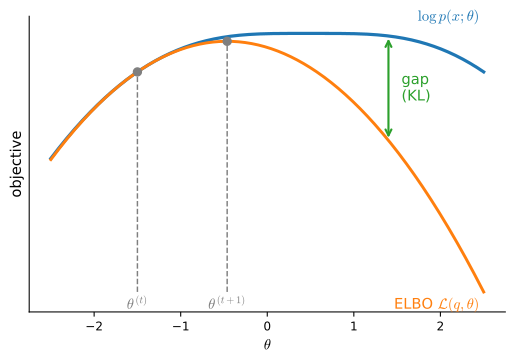
For the point \(x=0.5\) of the previous subsection, the log-evidence is \(\log p(x)=-1.42\). The lazy guess \(q=(\tfrac12,\tfrac12)\) gives an ELBO of \(-1.54\), and the missing \(0.12\) nats are the KL divergence from \((\tfrac12,\tfrac12)\) to the posterior \((0.27,0.73)\). The bound falls short by the distance of the guess from the posterior, and by nothing else. Figure 36.7.1 draws the bound as a function of the parameters.
36.7.3 Expectation–Maximization
The proposition turns the hard problem into coordinate ascent on \(\mathcal{L}(q, \boldsymbol{\theta})\): maximize over one of the two arguments while holding the other fixed, then swap, and repeat. For a data set \(X = \{x_1,\ldots,x_n\}\) of independent observations the bound applies example by example and sums, with one guess \(q_i\) per data point. The expectation–maximization (EM) algorithm alternates the two coordinates (Dempster et al. 1977):
E-step. Hold \(\boldsymbol{\theta}^{(t)}\) fixed and maximize over the guesses. By the equality condition of Equation 36.7.3, the best \(q_i\) is the posterior, \(q_i^{(t)}(z) = p(z \mid x_i, \boldsymbol{\theta}^{(t)})\). This closes every gap and makes the bound tight: \(\sum_i \mathcal{L}(q_i^{(t)}, \boldsymbol{\theta}^{(t)}) = \log P(X\mid\boldsymbol{\theta}^{(t)})\).
M-step. Hold the guesses fixed and maximize over the parameters:
\[ \boldsymbol{\theta}^{(t+1)} = \mathop{\mathrm{argmax}}_{\boldsymbol{\theta}} \sum_i \mathbb{E}_{q_i^{(t)}}\big[\log p(x_i, z\mid\boldsymbol{\theta})\big], \]
since the entropy terms do not involve \(\boldsymbol{\theta}\). This is the easy complete-data objective, with soft assignments standing in for the oracle’s labels.
Proposition (EM never decreases the likelihood). Each EM iteration satisfies \(\log P(X\mid\boldsymbol{\theta}^{(t+1)}) \ge \log P(X\mid\boldsymbol{\theta}^{(t)})\).
Proof. Chain three facts:
\[ \log P(X\mid\boldsymbol{\theta}^{(t+1)}) \;\ge\; \sum_i \mathcal{L}\big(q_i^{(t)}, \boldsymbol{\theta}^{(t+1)}\big) \;\ge\; \sum_i \mathcal{L}\big(q_i^{(t)}, \boldsymbol{\theta}^{(t)}\big) \;=\; \log P(X\mid\boldsymbol{\theta}^{(t)}). \]
The first inequality is the ELBO bound Equation 36.7.2 at the new parameters; the second is the definition of the M-step; the equality is the tightness that the E-step achieved. \(\blacksquare\)
For the Gaussian mixture both steps have closed forms. The E-step computes the responsibilities, the posterior probability that point \(i\) came from component \(k\), as in the hand computation above,
\[ r_{ik} = \frac{\pi_k\, \mathcal{N}(x_i;\, \mu_k, \sigma_k^2)} {\sum_{j} \pi_j\, \mathcal{N}(x_i;\, \mu_j, \sigma_j^2)}. \]
The M-step refits each component by responsibility-weighted counting and averaging. With effective counts \(n_k = \sum_i r_{ik}\),
\[ \pi_k = \frac{n_k}{n}, \qquad \mu_k = \frac{1}{n_k}\sum_{i} r_{ik}\, x_i, \qquad \sigma_k^2 = \frac{1}{n_k}\sum_{i} r_{ik}\,(x_i - \mu_k)^2. \tag{36.7.4}\]
These are the complete-data estimators, the fraction, the mean and the variance, softened: instead of voting for one component, each point spreads its single vote across the components in proportion to its responsibilities. If all components share one fixed variance \(\sigma^2\) and we let \(\sigma^2\to0\), the responsibilities become hard assignments to the nearest mean, and EM becomes the K-means algorithm.
The two steps fit in a dozen lines. We draw \(300\) points from \(\mathcal N(-2, 0.8^2)\) and \(200\) from \(\mathcal N(1.5, 0.6^2)\), and implement EM for a mixture of \(K\) Gaussians in one dimension; em returns the log-likelihood at every step together with the final parameters.
The proposition says that the trace cannot go down. It says nothing about speed. We start from a poor guess, two heavily overlapping components at \(\pm0.5\) with unit scale, run \(30\) steps, and print the first six values and the last.
lls, pi, mu, sigma = em(x, [0.5, 0.5], [-0.5, 0.5], [1, 1], 30)
print('steps 0-5:', lls[:6].round(1), ' step 29:', lls[-1].round(1))
print(f'pi = {pi.round(2)}, mu = {mu.round(2)}, sigma = {sigma.round(2)}')steps 0-5: [-1298.1 -989.9 -942. -871. -848.6 -847. ] step 29: -846.8
pi = [0.59 0.41], mu = [-2.04 1.54], sigma = [0.74 0.6 ]steps 0-5: [-1271.8 -985.3 -945.7 -878.5 -845.1 -842.3] step 29: -842.2
pi = [0.6 0.4], mu = [-2.01 1.5 ], sigma = [0.75 0.57]steps 0-5: [-1252.9 -984.7 -953.8 -901. -868.5 -862.7] step 29: -861.4
pi = [0.6 0.4], mu = [-1.94 1.5 ], sigma = [0.82 0.55]steps 0-5: [-1315.3 -992.9 -945.5 -876.4 -856. -854. ] step 29: -853.5
pi = [0.6 0.4], mu = [-2.07 1.54], sigma = [0.76 0.6 ]The log-likelihood climbs by more than \(400\) nats, from about \(-1{,}300\) to between \(-850\) and \(-890\) (the exact values depend on the draw). Nearly all of the climb happens at once: after six steps the trace is within about a nat of its final value. The recovered weights, means, and scales lie within about \(0.2\) of the generating values \((0.6, 0.4)\), \((-2, 1.5)\), and \((0.8, 0.6)\).
EM has four limits. The first is harmless. Relabeling the \(K\) components gives \(K!\) equally good copies of every maximum. This label switching is the same non-identifiability as permuting the hidden units of a network, and it makes no maximum worse than another.
The second limit is that EM stops at the first stationary point it reaches. A symmetric start makes the point. Before running the cell, predict what EM does when both components begin with the same mean and scale.
lls2, pi2, mu2, sigma2 = em(x, [0.5, 0.5], [0, 0], [1, 1], 30)
print(f'log-likelihood {lls2[0]:.1f} -> {lls2[-1]:.1f}, '
      f'{lls[-1] - lls2[-1]:.1f} below the previous fit')
print(f'pi = {pi2.round(2)}, mu = {mu2.round(2)}, sigma = {sigma2.round(2)}')
print(f'mean of x = {x.mean():.2f}, standard deviation of x = {x.std():.2f}')log-likelihood -1438.7 -> -1027.5, 180.7 below the previous fit
pi = [0.5 0.5], mu = [-0.59 -0.59], sigma = [1.89 1.89]
mean of x = -0.59, standard deviation of x = 1.89log-likelihood -1405.6 -> -1017.8, 175.7 below the previous fit
pi = [0.5 0.5], mu = [-0.59 -0.59], sigma = [1.85 1.85]
mean of x = -0.59, standard deviation of x = 1.85log-likelihood -1381.5 -> -1012.9, 151.5 below the previous fit
pi = [0.5 0.5], mu = [-0.57 -0.57], sigma = [1.83 1.83]
mean of x = -0.57, standard deviation of x = 1.83log-likelihood -1459.2 -> -1030.5, 176.9 below the previous fit
pi = [0.5 0.5], mu = [-0.62 -0.62], sigma = [1.9 1.9]
mean of x = -0.62, standard deviation of x = 1.90The two components never separate. Their responsibilities are equal for every point, so the M-step keeps them identical, and EM settles on the single-Gaussian fit, the overall mean and standard deviation of the data, more than \(100\) nats below the two-cluster solution. Every fixed point of EM is a stationary point of the likelihood, not necessarily a maximum, so in practice EM is restarted from several random initializations. Random initialization breaks the same symmetry among the hidden units of a layer (Section 4.4): units that start equal receive equal gradients and stay equal.
The third limit is that the mixture likelihood is unbounded. Put the second component on the first data point, \(\mu_2=x_1\), with weight \(\pi_2=1/n\) and scale \(\epsilon\). Its density at \(x_1\) is \(\tfrac1n(2\pi)^{-1/2}\epsilon^{-1}\), while the first component still explains the other points, so
\[ \ell(\boldsymbol{\theta}) \le \log\big(n\sqrt{2\pi}\big) + \log\epsilon + \textrm{const}, \]
where the constant collects the other \(n-1\) points. As \(\epsilon\to0\) the NLL goes to \(-\infty\): the maximum likelihood “solution” is a spike on one data point. A floor on the variances, or a prior on them, removes the spike. With the set of parameters at least as good as the starting point then compact, every limit point of EM is a stationary point of the floored problem (Wu 1983).
The fourth limit is that the monotonicity proof needs the exact posterior in the E-step, and approximate E-steps lose the guarantee. A variational autoencoder (Kingma and Welling 2014) keeps the ELBO but replaces the per-point posterior by a neural network \(q_{\boldsymbol{\phi}}(z\mid x)\), trained jointly with the generator, because for a deep decoder the posterior has no closed form. It climbs the bound by stochastic gradients rather than by exact EM steps. Here the bound outgrows the algorithm that introduced it. The latent variable need not be a cluster label. Put the parameters themselves in its place, and the posterior that the E-step asks for is the posterior over parameters, the object that Section 36.6 ended by asking for. It is rarely available either, and Section 36.8 is about what can be computed instead.
36.7.4 Summary
With hidden variables, the likelihood has a sum inside its logarithm, and the fit that would be counting and averaging if the variables were observed has no closed form. A probabilistic guess \(q\) for the hidden variables restores the easy problem as a lower bound: the ELBO lies below the log-evidence by the KL divergence from \(q\) to the posterior of the latent variable. EM alternates between closing that gap and climbing the bound. It never decreases the likelihood, but it stops at the first stationary point it reaches, and the mixture likelihood needs a floor on the variances to have a maximum at all.
36.7.5 Exercises
- [code] EM speed and missing information. ● Consider the mixture \(p(x\mid\pi)=\pi f_0(x)+(1-\pi)f_1(x)\) with known components \(f_0=\mathcal N(\cdot\,;0,1)\) and \(f_1=\mathcal N(\cdot\,;\Delta,1)\), in which only the weight \(\pi\) is unknown.
Show that EM updates the weight by \(\pi^{(t+1)}=M(\pi^{(t)})\) with \(M(\pi)=\tfrac1n\sum_i r_i(\pi)\) and responsibilities \(r_i(\pi)=\pi f_0(x_i)/p(x_i\mid\pi)\).
Near a fixed point \(\hat\pi=M(\hat\pi)\), each iteration multiplies the error by about \(M'(\hat\pi)\). Define the observed information \(I_{\textrm{obs}}=-\frac{d^2}{d\pi^2}\sum_i\log p(x_i\mid\pi)\) at \(\hat\pi\), and the complete-data information \(I_{\textrm{com}}=n/(\hat\pi(1-\hat\pi))\) that the labels would carry if they were observed (compare Equation 36.6.6). Show that
\[M'(\hat\pi)=1-\frac{I_{\textrm{obs}}}{I_{\textrm{com}}}. \tag{36.7.5}\]
Express both sides through the responsibilities and use \(\sum_i r_i(\hat\pi)=n\hat\pi\). Dempster et al. (1977) prove the general form of this result: the rate of EM is set by the fraction of the information that the latent variables hide.
Draw \(n=10{,}000\) points with \(\pi=0.3\) for each \(\Delta\in\{0.5,1,2,4\}\), run EM from \(\pi^{(0)}=0.5\), and compare the measured ratio of successive errors with the prediction of (b). With \(\hat\pi\) taken from a long run, how many iterations does each \(\Delta\) need to bring the error below \(10^{-6}\)?
What does the ratio \(I_{\textrm{obs}}/I_{\textrm{com}}\) say about the standard error of \(\hat\pi\), compared with a data set of the same size whose labels were observed?
- The bound by hand. Take the single observation \(x=0.5\) and the two equally weighted components \(\mathcal N(-1,1)\) and \(\mathcal N(1,1)\) of the text.
- Compute \(\log p(x)\), and the ELBO Equation 36.7.2 for the guess \(q=(\tfrac12,\tfrac12)\) and for the posterior \(q=(0.27,0.73)\). Check the two values quoted in the text.
- Verify Equation 36.7.3 for the uniform guess by computing the KL divergence directly.
- A hard guess puts all of \(q\) on the right component. Compute its ELBO and its gap. An algorithm that alternates hard guesses with M-steps still never decreases the ELBO. Why is its likelihood no longer guaranteed to increase?
- K-means as a limit. Let all \(K\) components of a Gaussian mixture have equal weights and one fixed variance \(\sigma^2\), so that only the means are fitted.
- Write the responsibilities \(r_{ik}\) as a softmax of \(-(x_i-\mu_k)^2/(2\sigma^2)\) over \(k\). What plays the role of the temperature? Show that, as \(\sigma^2\to0\), the responsibility of the nearest mean tends to \(1\) whenever the nearest mean is unique.
- Show that the M-step Equation 36.7.4 then sets each mean to the average of the points assigned to it, and that the two steps together never increase \(\sum_i (x_i-\mu_{z_i})^2\), where \(z_i\) is the component assigned to point \(i\).
- In the symmetric start of the text, both means begin at the same place. What does K-means do from such a start, and what does this say about the tie-breaking rule of an implementation?