%matplotlib inline
from d2l import torch as d2l
import torch
from torch import nn
from torch.nn import functional as F

torch.set_float32_matmul_precision('high')13.5 Multi-GPU from First Principles
Adding GPUs increases aggregate arithmetic and memory capacity. This section builds data-parallel training explicitly, with device-to-device copies and a hand-written gradient sum, so that the production mechanisms in Section 13.6 are clear. We derive ring allreduce and its communication cost. Because the build machine has no fast inter-GPU fabric, the experiments also show when communication or reduced per-device utilization prevents speedup.
The experimental machine has neither NVLink nor peer-to-peer transfer (Section 13.2). A faster fabric reduces the communication term but does not remove it. Since the derivation treats the number of devices as a variable, the same cost model applies beyond this machine.
Prerequisites: minibatch SGD and the effect of batch size on the gradient estimate (@sec-minibatch-sgd); LeNet (@sec-lenet); the interconnect measurements of Section 13.2.5.
%matplotlib inline
from d2l import jax as d2l
import jax
from jax import numpy as jnp
import numpy as np
import optax
import os
from functools import partial

# XLA's NCCL buffer registration fails harmlessly on this P2P-less box;
# opt out rather than let every collective print the warning.
os.environ.setdefault('NCCL_LOCAL_REGISTER', '0')'0'13.5.1 Three Ways to Split
Given more than one GPU and a model to train, there are three ways to divide the work (Figure 13.5.1).
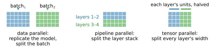
Data parallelism replicates the whole model on every GPU and splits the batch: each device runs the full network on a different slice of the minibatch, then the devices sum their gradients so every replica takes the same optimizer step. It is the simplest, works for any model that fits on one GPU, and needs communication only once per step — so it is what this chapter builds. Pipeline parallelism splits the layer stack across devices, each holding a few consecutive layers; it lets a model too deep for one GPU fit, at the cost of tight inter-stage synchronization. Tensor parallelism splits within each layer — each device holds a slice of every weight matrix — and communicates several times per layer. The latter two matter only at scales this part defers to the Language Models chapters, which have models large enough to warrant them; a single historical note is that the very first of them appeared in 2012, when AlexNet was split across two GPUs because its weights did not fit in one card’s 3 GB (Krizhevsky et al. 2012). Data parallelism is our subject, and it does not let you train a bigger model, a warning that Section 13.4 already made: every GPU still holds a full copy.
13.5.2 Data Parallelism by Hand
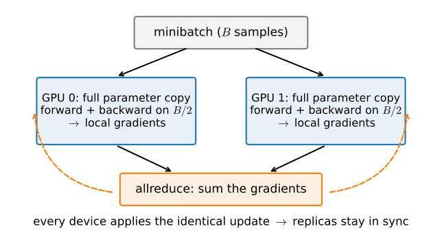
Data-parallel training on \(k\) GPUs is five steps per minibatch: split the batch into \(k\) shards; run forward and backward on each shard against that device’s copy of the parameters; sum the \(k\) gradient sets so all devices agree; and let every device apply the same update (Figure 13.5.2). We build each piece for a small LeNet, then run it — and watch the second GPU buy us nothing.
We define LeNet from raw tensors (not a module) so that parameters, gradients, and their movement between devices are fully visible:
scale = 0.01
def new_params(device):
    def p(*shape):
        return (torch.randn(*shape, device=device) * scale).requires_grad_()
    return [p(20, 1, 3, 3), torch.zeros(20, device=device, requires_grad=True),
            p(50, 20, 5, 5), torch.zeros(50, device=device, requires_grad=True),
            p(800, 128), torch.zeros(128, device=device, requires_grad=True),
            p(128, 10), torch.zeros(10, device=device, requires_grad=True)]

def lenet(X, params):
    h1 = F.avg_pool2d(F.relu(F.conv2d(X, params[0], params[1])), 2, 2)
    h2 = F.avg_pool2d(F.relu(F.conv2d(h1, params[2], params[3])), 2, 2)
    h2 = h2.reshape(h2.shape[0], -1)
    h3 = F.relu(torch.mm(h2, params[4]) + params[5])
    return torch.mm(h3, params[6]) + params[7]

loss = nn.CrossEntropyLoss(reduction='none')
scale = 0.01
def new_params(key):
ks = jax.random.split(key, 4)
return [jax.random.normal(ks[0], (20, 1, 3, 3)) * scale, jnp.zeros(20),
jax.random.normal(ks[1], (50, 20, 5, 5)) * scale, jnp.zeros(50),
jax.random.normal(ks[2], (800, 128)) * scale, jnp.zeros(128),
jax.random.normal(ks[3], (128, 10)) * scale, jnp.zeros(10)]
def lenet(params, X):
conv = lambda x, W: jax.lax.conv_general_dilated(
x, W, (1, 1), 'VALID', dimension_numbers=('NCHW', 'OIHW', 'NCHW'))
pool = lambda x: jax.lax.reduce_window(
x, 0.0, jax.lax.add, (1, 1, 2, 2), (1, 1, 2, 2), 'VALID') / 4.0
h1 = pool(jax.nn.relu(conv(X, params[0]) + params[1].reshape(1, -1, 1, 1)))
h2 = pool(jax.nn.relu(conv(h1, params[2]) + params[3].reshape(1, -1, 1, 1)))
h2 = h2.reshape(h2.shape[0], -1)
h3 = jax.nn.relu(jnp.dot(h2, params[4]) + params[5])
return jnp.dot(h3, params[6]) + params[7]The two operations that make it parallel are broadcasting parameters to each device and summing gradients across them. We build the PyTorch version by hand, because the hand-rolled version is the lesson; the #@saved split_batch (which chops a minibatch into per-device shards) rounds out the toolkit:
def get_params(params, device):
    return [p.clone().to(device).detach().requires_grad_() for p in params]

def allreduce(data):
    # Star pattern: sum everything onto device 0, then broadcast back.
    for i in range(1, len(data)):
        data[0][:] += data[i].to(data[0].device)
    for i in range(1, len(data)):
        data[i][:] = data[0].to(data[i].device)

def split_batch(X, y, devices):
    """Split `X` and `y` into multiple devices."""
    assert X.shape[0] == y.shape[0]
    return (nn.parallel.scatter(X, devices),
            nn.parallel.scatter(y, devices))
def get_params(params, num_devices):
"""Data parallelism replicates the full parameter set on every device;
shard_map's P() in-spec (below) broadcasts one copy to each."""
return params
def split_batch(X, y, num_devices):
"""Reshape `X` and `y` onto a leading device axis of size num_devices."""
assert X.shape[0] % num_devices == 0
reshape = lambda a: a.reshape(num_devices, -1, *a.shape[1:])
return reshape(X), reshape(y)allreduce is the central operation. The implementation above uses a simple star topology: it gathers every device’s gradient onto device 0, sums there, and broadcasts back, with device 0 as a hub that handles all \(k-1\) inbound and \(k-1\) outbound transfers. Watch it work on two vectors living on two GPUs:
data = [torch.ones((1, 2), device=d2l.try_gpu(i)) * (i + 1)
        for i in range(min(2, d2l.num_gpus()))]
print('before:', [d.cpu().numpy().tolist() for d in data])
allreduce(data)
print('after: ', [d.cpu().numpy().tolist() for d in data])
before: [[[1.0, 1.0]], [[2.0, 2.0]]]
after: [[[3.0, 3.0]], [[3.0, 3.0]]]# JAX writes the same allreduce as a collective inside shard_map (below,
# a pmean: the sum divided by k); here we show the summed result it is
# built on.
data = jnp.stack([jnp.ones((1, 2)) * (i + 1)
for i in range(min(2, jax.local_device_count()))])
print('before:', data.tolist())
print('summed:', jnp.broadcast_to(data.sum(0), data.shape).tolist())before: [[[1.0, 1.0]], [[2.0, 2.0]]]
summed: [[[3.0, 3.0]], [[3.0, 3.0]]]The training step assembles the pieces. Each device computes its shard’s gradient; we allreduce parameter by parameter; each device applies plain SGD. This implementation runs in one Python process because it moves tensors explicitly:
def train_batch(X, y, device_params, devices, lr):
    X_shards, y_shards = split_batch(X, y, devices)
    ls = [loss(lenet(Xs, dev_W), ys).sum()
          for Xs, ys, dev_W in zip(X_shards, y_shards, device_params)]
    for l in ls:
        l.backward()
    with torch.no_grad():
        for i in range(len(device_params[0])):
            allreduce([device_params[c][i].grad for c in range(len(devices))])
        for param in device_params:
            d2l.sgd(param, lr, X.shape[0])
            for p in param:
p.grad = None@partial(jax.jit, static_argnames=('lr', 'mesh'))
def train_step(params, X, y, lr, mesh):
"""One data-parallel step: shard_map makes the pmean collective explicit.
`X`, `y` arrive with the batch sharded across devices (P('data')) and
`params` replicated (P()) -- see `train` below; shard_map hands each device
the full parameter replica and its own batch shard. pcast marks the replica
as this device's own local copy, so the gradient below is the shard's own;
pmean then averages the shard gradients across devices."""
P = jax.sharding.PartitionSpec
def per_device(params, X, y):
def loss_fn(p):
logits = lenet(p, X[0]) # X[0]: strip the size-1 sharded axis
return optax.softmax_cross_entropy_with_integer_labels(
logits, y[0]).mean()
local = jax.lax.pcast(params, 'data', to='varying') # my own copy
grads = jax.grad(loss_fn)(local) # my shard's mean-loss gradient
grads = jax.lax.pmean(grads, 'data') # The allreduce, in one line
return jax.tree.map(lambda p, g: p - lr * g, params, grads)
step = jax.shard_map(per_device, mesh=mesh,
in_specs=(P(), P('data'), P('data')),
out_specs=P())
return step(params, X, y)The two tabs make the same computation visible in two idioms. PyTorch moves gradients between devices with explicit .to(device) copies inside allreduce; JAX writes the collective as a single jax.lax.pmean inside a jax.shard_map, where the PartitionSpec('data') annotation tells XLA that the leading axis is sharded across devices. (Note the top-level jax.shard_map — the older jax.pmap is a compatibility shim as of JAX 0.8 and we do not use it.) The JAX tab requires one additional distinction: under shard_map the parameters arrive replicated, and differentiating a replicated tensor makes JAX’s autodiff insert a gradient sum of its own — the transpose of “broadcast to every device” is “add up every device’s contribution”, and a further explicit psum on top would then double-count. The pcast(..., to='varying') line opts out by declaring each replica device-local, so the code owns the collective: every device takes its shard’s mean-loss gradient, and pmean averages them into exactly the gradient one device would compute on the whole batch. The collective is visible in both tabs, which is the purpose of this manual implementation.
Both tabs claim that \(k\) devices take the same step as one device. The following parity check verifies this claim. From the same initialization and minibatch, one step on two GPUs must move the parameters exactly where one step on one GPU does. The test is cheap, and it catches normalization bugs that no accuracy curve reliably reveals, such as a summed instead of averaged gradient acting as an accidental \(k\times\) learning rate:
X, y = torch.randn(256, 1, 28, 28), torch.randint(0, 10, (256,))
base = new_params(d2l.try_gpu(0))
deltas = []
for k in (1, min(2, d2l.num_gpus())):
    devices = [d2l.try_gpu(i) for i in range(k)]
    device_params = [get_params(base, d) for d in devices]
    train_batch(X, y, device_params, devices, lr=0.2)
    deltas.append([(p - b).detach().cpu()
                   for p, b in zip(device_params[0], base)])
print('max update difference, k=1 vs k=2: '
      f'{max((a - b).abs().max() for a, b in zip(*deltas)):.2e}')
max update difference, k=1 vs k=2: 9.31e-10P = jax.sharding.PartitionSpec
X = jax.random.normal(jax.random.PRNGKey(1), (256, 1, 28, 28))
y = jax.random.randint(jax.random.PRNGKey(2), (256,), 0, 10)
base = new_params(jax.random.PRNGKey(0))
deltas = []
for k in (1, min(2, jax.local_device_count())):
mesh = jax.make_mesh((k,), ('data',))
place = lambda a, spec: jax.device_put(
a, jax.sharding.NamedSharding(mesh, spec))
params = jax.tree.map(lambda p: place(p, P()), base)
Xs, ys = split_batch(X, y, k)
new = train_step(params, place(Xs, P('data')), place(ys, P('data')),
0.2, mesh)
deltas.append([np.asarray(n - b) for n, b in zip(new, base)])
print('max update difference, k=1 vs k=2: '
f'{max(np.abs(a - b).max() for a, b in zip(*deltas)):.2e}')max update difference, k=1 vs k=2: 1.86e-09The parameter updates agree to floating-point noise — around \(10^{-9}\), against update magnitudes near \(10^{-2}\). “Mathematically identical” is now a measurement, not a slogan. With correctness established, the training loop that wraps train_batch/train_step is the multi-GPU cousin of Section 6.6’s. First, one GPU:
def train(num_gpus, batch_size, lr):
    train_iter, test_iter = d2l.load_data_fashion_mnist(batch_size)
    devices = [d2l.try_gpu(i) for i in range(num_gpus)]
    base = new_params(devices[0])
    device_params = [get_params(base, d) for d in devices]
    timer, num_epochs = d2l.Timer(), 5
    for epoch in range(num_epochs):
        timer.start()
        for X, y in train_iter:
            train_batch(X, y, device_params, devices, lr)
        for d in devices:   # completion timing: sync before stopping the clock
            torch.cuda.synchronize(d)
        timer.stop()
    acc = d2l.evaluate_accuracy_gpu(
        lambda x: lenet(x, device_params[0]), test_iter, devices[0])
    print(f'test acc {acc:.2f}, {timer.avg():.2f} sec/epoch on {num_gpus} GPU(s)')

train(num_gpus=1, batch_size=256, lr=0.2)
test acc 0.70, 2.37 sec/epoch on 1 GPU(s)def train(num_gpus, batch_size, lr):
P = jax.sharding.PartitionSpec
data = d2l.FashionMNIST(batch_size=batch_size)
train_iter = data.get_dataloader(train=True)
mesh = jax.make_mesh((num_gpus,), ('data',))
place = lambda a, spec: jax.device_put(
a, jax.sharding.NamedSharding(mesh, spec))
params = get_params(new_params(jax.random.PRNGKey(0)), num_gpus)
params = jax.tree.map(lambda p: place(p, P()), params) # a replica per device
timer, num_epochs = d2l.Timer(), 5
for epoch in range(num_epochs):
timer.start()
for X, y in train_iter:
X = jnp.array(X).transpose(0, 3, 1, 2)
if X.shape[0] % num_gpus: # drop a ragged final batch
continue
Xs, ys = split_batch(X, jnp.array(y), num_gpus)
Xs, ys = place(Xs, P('data')), place(ys, P('data')) # shard the batch
params = train_step(params, Xs, ys, lr, mesh)
jax.block_until_ready(params)
timer.stop()
apply_fn, hits, total = jax.jit(lenet), 0, 0
p0 = jax.tree.map(lambda p: jax.device_put(p, jax.devices()[0]), params)
for X, y in data.get_dataloader(train=False):
X = jnp.array(X).transpose(0, 3, 1, 2)
hits += int((apply_fn(p0, X).argmax(axis=1) == jnp.array(y)).sum())
total += len(y)
print(f'test acc {hits / total:.2f}, {timer.avg():.2f} sec/epoch '
f'on {num_gpus} GPU(s)')
train(num_gpus=1, batch_size=256, lr=0.2)test acc 0.79, 0.55 sec/epoch on 1 GPU(s)Now two GPUs, same batch size and learning rate. The optimization is mathematically identical, as the one-step check just proved — any accuracy gap between these short runs is run-to-run noise from initialization and rounding, not the parallelism — but the wall-clock is no better:
train(num_gpus=min(2, d2l.num_gpus()), batch_size=256, lr=0.2)test acc 0.79, 2.31 sec/epoch on 2 GPU(s)train(num_gpus=min(2, jax.local_device_count()), batch_size=256, lr=0.2)test acc 0.80, 0.90 sec/epoch on 2 GPU(s)The second GPU buys no speedup — on our box the two-GPU run is at best on par with one GPU and is slower in JAX, as expected when each device is underutilized. The reason is not slow communication: LeNet’s parameters are tiny — the whole gradient set is about half a megabyte — so its allreduce is negligible, and we measure the transport directly below. LeNet is too small for data parallelism to improve throughput. Splitting a 256-example batch into two 128-example shards underfeeds each GPU — a convolution on half the batch does not run at half the time, because a small batch never filled the device to begin with — and the Python orchestration and per-step dispatch are not amortized by microsecond-scale compute. The technique is not wrong; the regime is wrong. This tiny model is the worst case for data parallelism, and diagnosing exactly why is the next two subsections’ work: separating the communication cost, which is small here, from the underutilization cost, which is not.
13.5.3 Ring Allreduce
Our star allreduce uses device 0 as a hub for all transfers. It moves \((k-1)N\) bytes in and \((k-1)N\) out for a parameter set of \(N\) bytes, and the other devices’ links sit idle while it works. Ring allreduce (Patarasuk and Yuan 2009) removes this hub. Its two phases also provide the basis for FSDP in Section 13.6.
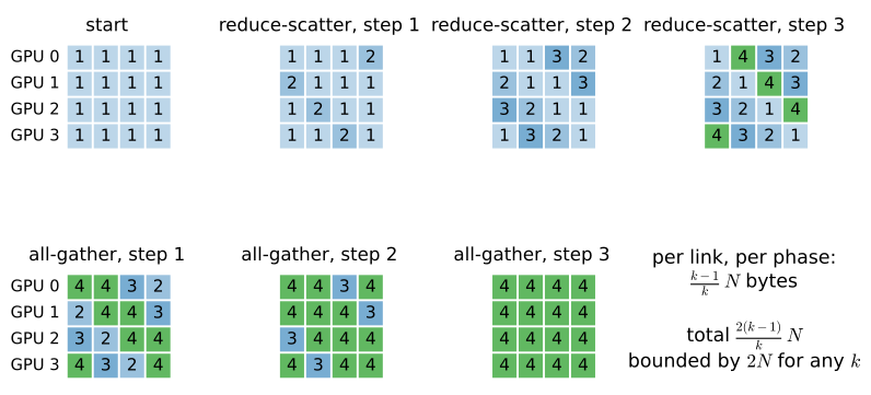
Arrange the \(k\) devices in a ring, each talking only to its neighbor. Split each device’s gradient vector into \(k\) equal chunks. The allreduce runs in two phases (Figure 13.5.3). In reduce-scatter, over \(k-1\) steps, device \(i\) sends one chunk to its neighbor while receiving and accumulating another; after the phase, each device owns one fully-summed chunk (a different chunk per device). In all-gather, another \(k-1\) steps pass those finished chunks around the ring until every device has all \(k\). At every step, every link carries exactly one chunk of size \(N/k\), so each device sends \((k-1) \cdot N/k\) bytes per phase, and both phases together move
\[ \frac{2(k-1)}{k}\, N \quad\text{bytes per device,} \tag{13.5.1}\]
which is nearly constant in \(k\): it rises from \(N\) at \(k=2\) toward its bound of \(2N\) and never exceeds it, however many devices join the ring. The star pattern’s hub moved \((k-1)N\) — linear in \(k\); the ring moves at most \(2N\). That is why production collective libraries are built on rings and trees, chosen per message size and topology, alongside hardware-specific schemes; for messages small enough that per-hop latency dominates the byte count, trees win — a term this byte-only accounting deliberately ignores.
The \(2(k-1)/k\) byte count does not determine the transfer rate. On the build machine, peer-to-peer transfer is unavailable, so each nominal peer-to-peer transfer, every “neighbor to neighbor” hop is really a round trip through host memory (Section 13.2.5), so the ring hop is staged through host memory (Section 13.2.5). The resulting transport bandwidth largely removes the ring’s theoretical advantage over a star. NCCL may still select a ring or tree by message size, but measured link bandwidth supplies the constant in the cost model.
13.5.4 Communication Cost and Scaling
We can now estimate whether another device reduces step time. One step on \(k\) GPUs takes roughly
\[ t_{\text{step}}(k) \;\approx\; \underbrace{t_{\text{compute}}(B/k)}_{\text{forward+backward on a shard}} \;+\; \underbrace{t_{\text{comm}}}_{\approx\, 2N / \beta}, \tag{13.5.2}\]
where \(B\) is the global batch, \(N\) the bytes of gradients to reduce, and \(\beta\) the achievable allreduce bandwidth (Equation 13.5.1 gives the \(2N\); the per-device traffic is bounded by it for any \(k\)). The compute term shrinks with more GPUs (each does less of the batch); the communication term does not. Parallelism pays exactly when the compute you offload exceeds the communication you take on — models with high compute per byte of gradient traffic, large per-device batches, and fast links all push in your favor; a tiny model on a slow link, like LeNet on the build machine, is a case where the second device does not improve time.
Two scaling conventions deserve names here, because every published speedup quietly picks one. Equation 13.5.2 holds the global batch \(B\) fixed while \(k\) grows — strong scaling: the same work, hopefully finishing sooner. The alternative holds the per-device batch fixed, so the global batch grows to \(kB_{\textrm{device}}\) — weak scaling: more work per unit time, quoted as throughput. The throughput sweep of Section 13.6 holds the per-rank batch fixed and must be read under the weak-scaling convention — and remember that a grown global batch changes the optimization trajectory itself (Section 9.10).
Let’s plug in real numbers by measuring \(\beta\) directly. One bookkeeping convention first, so the numbers below are comparable: we quote bytes moved per device per allreduce (\(\approx 2N\) for the ring) divided by wall-clock time — an effective bandwidth. NCCL’s benchmark “busbw” normalizes differently, so its figures are not directly comparable to ours. Here is the effective bandwidth of the allreduce each tab actually runs — the hand-rolled star in PyTorch, XLA’s psum collective in JAX:
if d2l.num_gpus() >= 2:
    N = 64 * 1024 * 1024  # 64M floats = 256 MB per replica
    data = [torch.randn(N, device=d2l.try_gpu(i)) for i in range(2)]
    t = d2l.Benchmark(lambda: allreduce(data), warmup=2, repeats=5).time
    # Per-device traffic is ~2N bytes; report effective bandwidth
    print(f'allreduce {2 * N * 4 / t / 1e9:.2f} GB/s effective '
          f'over {1000 * t:.1f} ms')
else:
    print('needs 2 GPUs')
allreduce 17.28 GB/s effective over 31.1 msif jax.local_device_count() >= 2:
mesh = jax.make_mesh((2,), ('data',))
P = jax.sharding.PartitionSpec
N = 64 * 1024 * 1024
x = jax.device_put(jnp.ones((2, N)),
jax.sharding.NamedSharding(mesh, P('data')))
psum = jax.jit(jax.shard_map(
lambda a: jax.lax.psum(a, 'data'), mesh=mesh,
in_specs=P('data'), out_specs=P('data')))
t = d2l.Benchmark(lambda: psum(x), warmup=2, repeats=5).time
print(f'psum {2 * N * 4 / t / 1e9:.2f} GB/s effective over {1000*t:.1f} ms')
else:
print('needs 2 GPUs')psum 2.71 GB/s effective over 198.2 msThe hand-rolled copy sustains roughly twenty GB/s — this is a plain PCIe transfer, staged through host memory, running near the bus limit, and two orders of magnitude below an NVLink domain’s ~1.8 TB/s per GPU (Table 13.2.1). This result also shows that a collective library such as NCCL, whose ring/tree chunking is tuned for peer-to-peer fabrics, extracts noticeably less effective bandwidth than this naive one-shot copy on our P2P-less box — its busbw here is only a couple of GB/s. The physical link is not limiting: our copy and NCCL cross the same PCIe links. The difference is how the bytes move. With peer-to-peer unavailable, NCCL falls back to a shared-memory transport whose default mode drives the transfer with a GPU kernel issuing load/store instructions across the bus — a latency-bound path — while our .to() copy rides the GPU’s DMA copy engines, built for exactly this. One environment variable (NCCL_SHM_USE_CUDA_MEMCPY=1) switches NCCL’s fallback onto those same copy engines and recovers most of the gap on this box — a workaround for what is best read as a platform-specific performance bug, not a setting to copy blindly: Section 13.6 measures the roughly five-fold recovery — and shows why its training runs nonetheless keep the library’s defaults. The diagnosis is this chapter’s method in miniature: the ceiling was not the algorithm and not the wire but one stage of the transport — and you find the binding stage by measuring, not by trusting the library.
The measured psum sustains well under ten GB/s in our convention — more than two orders of magnitude below an NVLink domain’s ~1.8 TB/s per GPU (Table 13.2.1). That number is itself a theory-versus-practice lesson: XLA hands the collective to NCCL, whose ring/tree chunking is tuned for peer-to-peer fabrics, and on our P2P-less box every “neighbor” hop stages through host memory — so the tuned library lands well below the roughly twenty GB/s a naive one-shot .to() copy achieves (the PyTorch tab measures it). The physical link is not limiting — both paths cross the same PCIe links. The gap is in how the fallback transport moves bytes (a latency-bound GPU-kernel copy by default, rather than the DMA copy engines), and a single NCCL environment switch recovers most of it in bare collectives (the PyTorch tab takes this apart, and Section 13.6 measures the workaround — and its limits). The ceiling was one stage of the transport — found, as always in this chapter, by measuring.
Now read the cost model against what we measured. LeNet’s parameters are tiny, so \(2N/\beta\) is a fraction of a millisecond — the communication term is not what denies the speedup. The limiting factor is the other term: \(t_{\text{compute}}(B/k)\) does not actually fall like \(1/k\) for a small model, because halving an already-small batch leaves each GPU underutilized, so \(t_{\text{compute}}(B/2) \approx t_{\text{compute}}(B)\) and the second GPU provides no wall-clock reduction. Multiple devices improve throughput only when compute time decreases with the per-device batch — for a compute-dense network with a large per-device batch, where \(t_{\text{compute}}(B/k) \approx t_{\text{compute}}(B)/k\) dominates the small \(t_{\text{comm}}\). Section 13.6 tests this regime.
A closing word of history, because it names the lineage. Before synchronous ring allreduce won for dense training, large-scale learning organized this same communication through parameter servers: dedicated storage nodes exposed a push (accumulate my gradient) and pull (give me the current sum) interface, sharding the parameters across servers so aggregation bandwidth scaled with the fleet (Li et al. 2014). That push/pull abstraction is the authors’ own lineage, and it lives on today in recommender-system embedding tables (the territory of Chapter 23), where the parameters are too large and too sparse for every worker to hold a full replica — and, more broadly, wherever sparse or asynchronous state dominates the traffic. For dense training, collectives won; the modern production map is Section 30.6.
13.5.5 Summary
- Data parallelism replicates the model, splits the batch, sums gradients with an allreduce, and applies the identical update on every device. It is the simplest form of multi-GPU training and does not enlarge the model that fits.
- Built by hand, the gradient sum is a star: device 0 is a hub moving \((k-1)N\) bytes each way. Ring allreduce removes the hub — reduce-scatter then all-gather — moving \(2(k-1)/k \cdot N\) bytes per device: nearly constant, bounded by \(2N\) however many devices join. That identity reappears as the basis of FSDP.
- The cost model \(t_{\text{step}}(k) \approx t_{\text{compute}}(B/k) + 2N/\beta\) decides whether a GPU pays — but only when compute genuinely scales with the batch. It is a strong-scaling statement (fixed global batch); weak scaling fixes the per-device batch instead, and every quoted speedup picks one convention. LeNet is the deliberate worst case: its gradients are tiny (communication negligible), yet a second GPU buys no speedup because halving an already-small batch underutilizes each device, so \(t_{\text{compute}}(B/k)\) does not fall. A one-step k=1-versus-k=2 equality check proves the parallel step is the same mathematics before any timing is read. Inter-GPU bandwidth on this P2P-less box is PCIe-limited (tens of GB/s for a raw copy; far less through NCCL’s fallback transport at its defaults — a documented switch recovers most of it in bare collectives, and Section 13.6 measures both the workaround and its limits) — two to three orders of magnitude below an NVLink domain.
- Parameter servers (push/pull) organized this communication for the asynchronous, multi-machine era; synchronous collectives won for dense training, and the pattern survives in recsys embedding systems and wherever sparse or asynchronous state dominates.
13.5.6 Exercises
Data versus pipeline parallelism. Consider a stack of \(L\) fully connected layers of width \(d\), with fp32 weights and no biases, trained on two GPUs with minibatch size \(B\). Data parallelism allreduces the gradients of all weights. Two-stage pipeline parallelism
(Figure 13.5.1) places the first \(L/2\) layers on one GPU and the rest on the other, so the forward pass sends the \(B \times d\) activations at the cut to the second GPU and the backward pass returns their gradient.
- Count the bytes that cross between the two GPUs per step in each scheme, and evaluate both for \(L = 32\), \(d = 4096\), and \(B = 256\). For which relation between \(B\), \(L\), and \(d\) does data parallelism move fewer bytes?
- In the pipeline, each GPU idles while the other computes. To shorten the idle time, split the minibatch into \(m\) micro-batches (Huang et al. 2019). In the forward phase, the first GPU hands each micro-batch to the second as soon as it is done, so that the second GPU works on micro-batch \(j\) while the first works on micro-batch \(j+1\). The backward phase starts after the last forward pass and runs the same schedule from the second GPU to the first. Assume that every micro-batch takes the same time on each stage. Derive the fraction of the step during which each GPU idles, and evaluate it for \(m = 1\) and \(m = 8\).
Gradient normalization. Two recipes compute a data-parallel gradient from \(k\) shards of a minibatch of \(B\) examples. In recipe A, each device sums its per-example losses, the devices sum their gradients, and the update divides by \(B\). In recipe B, each device averages its per-example losses, and the devices average their gradients.
- Show that both recipes yield the gradient of the full-batch mean loss when every shard holds \(B/k\) examples.
- A language model averages its loss over tokens. Two shards with the same number of sequences hold 3000 and 1000 tokens. Find the weight that recipe B gives a token on each shard, relative to the weight the token has in the full-batch token mean.
- Modify recipe B so that it is exact for any shard sizes, and identify the extra quantity that the devices must communicate before the update.
Batch normalization across shards. Suppose that
lenetapplied batch normalization (Section 7.3) in training mode after each of its two convolutions and after its hidden dense layer, and that each device normalized with the statistics of its own shard.- Decide whether the parity check of Section 13.5.2 would still pass. Justify the decision by listing the quantities that each device computes from its own shard and checking for each of them whether the two-device step reproduces its one-device value.
- Find the per-channel quantities that the devices must exchange in the forward pass to reproduce the one-device statistics exactly. Count their bytes per step and compare them with the 0.5 MB of LeNet’s gradients.
Latency in the allreduce. ● The byte count of Equation 13.5.1 ignores the fixed cost of starting a transfer. Let one transfer of \(m\) bytes over a link take \(\alpha + m/\beta\).
- Derive the time \(t_{\text{ring}}\) of a ring allreduce of \(N\) bytes on \(k\) devices, and describe how each of its two terms behaves as \(k\) grows.
- A binary-tree allreduce sums up the tree and broadcasts back down. It takes \(2\log_2 k\) steps, each of which sends the full \(N\) bytes, so \[t_{\text{tree}} = 2\log_2 k \left(\alpha + \frac{N}{\beta}\right).\] For \(k = 8\), \(\alpha = 10\ \mu\textrm{s}\), and \(\beta = 20\) GB/s, find the message size below which the tree is faster than the ring.
- A data-parallel LeNet step that allreduces each of its eight parameter tensors separately, with the star pattern at \(k = 2\), makes 16 transfers. With the same \(\alpha\) and \(\beta\), estimate its communication time per step and the share of that time due to \(\alpha\). Repeat the estimate for a single allreduce of all gradients concatenated into one buffer.
Parameter servers and the ring. In the parameter-server design described at the end of Section 13.5.4, \(s\) server nodes each hold \(N/s\) bytes of the parameters (Li et al. 2014). In every step, each of \(k\) workers pushes its gradient for each slice to that slice’s server and then pulls the updated slice back.
- Count the bytes that each worker and each server send and receive per step. Find the number of servers at which a server’s link is no busier than a worker’s.
- Now let the \(k\) workers act as the servers, each holding \(1/k\) of the parameters. Show that the traffic of each device equals Equation 13.5.1, and match the push and pull phases to the two phases of ring allreduce.
Bandwidth conventions. The measurement in Section 13.5.4 reports \(2N/t\) for an allreduce of \(N\) bytes per device that takes time \(t\). The NCCL benchmarks report the algorithm bandwidth \(S/t\) for a message of \(S\) bytes and the bus bandwidth \[\textrm{busbw} = \frac{S}{t} \cdot \frac{2(k-1)}{k}. \tag{13.5.3}\]
- List the copies that the star pattern makes at \(k = 2\), and explain why \(2N/t\) is then the rate at which bytes cross the link.
- Express \(2N/t\) in terms of busbw, for \(k = 2\) and for general \(k\).
- A benchmark reports a busbw of 400 GB/s for an allreduce on eight GPUs. Predict the time to allreduce 1 GB of gradients, and find the relative error made by inserting the busbw as \(\beta\) into Equation 13.5.2.
Adapted from NVIDIA, Performance reported by NCCL tests, section “Bus bandwidth”.
Strong-scaling speedup. Model the compute time of a shard of \(b\) examples as \(t_{\text{compute}}(b) = t_0 + c\,b\), where \(t_0\) does not shrink with the shard. Let each device send at bandwidth \(\beta\), so that by Equation 13.5.1 one step at a fixed global batch \(B\) takes \[t_{\text{step}}(k) = t_0 + \frac{c\,B}{k} + \frac{2(k-1)}{k}\,\frac{N}{\beta}, \tag{13.5.4}\] with no communication at \(k = 1\). The strong-scaling speedup is \(S(k) = t_{\text{step}}(1) / t_{\text{step}}(k)\).
- Show that \(S(k) > 1\) holds for one \(k > 1\) exactly when it holds for every \(k > 1\), and find the condition. Find the limit of \(S(k)\) as \(k \to \infty\).
- A model with 11.2 million fp32 parameters has \(t_0 = 2\) ms and \(c = 0.2\) ms per example, and it is trained with \(B = 256\). Compute \(S(2)\), \(S(4)\), and the limit for \(\beta = 20\) GB/s and for \(\beta = 5\) GB/s. Find the bandwidth below which no number of GPUs speeds up this model.
- Sending the gradients in bf16 instead of fp32 halves \(N\). For \(\beta = 5\) GB/s, recompute \(S(4)\) and the limit of \(S(k)\), and state which of the two gains more from the halving.
[code] Gradients in bf16. ● Sending gradients in bf16 halves their bytes but rounds them. In a ring, each reduce-scatter hop adds the incoming partial sum to the local chunk, so a bf16 ring rounds the partial sum to bf16 once per hop.
- At the parameters returned by
new_params, compute the gradients ofleneton \(k\) disjoint Fashion-MNIST shards of 128 examples each, and flatten each shard’s gradients into one vector. Add the vectors one after another, rounding to bf16 after every addition, and measure the relative error of the result against an fp32 sum for \(k \in \{2, 8, 64\}\). Repeat with each vector rounded to bf16 once and the sum accumulated in fp32. Explain how each error depends on \(k\). - Compare the error at \(k = 8\) with the relative difference between the gradients of two shards, and decide whether the rounding matters for SGD.
- At the parameters returned by
[code] Strong and weak scaling of LeNet. ● Section 13.5.4 attributes LeNet’s missing speedup to \(t_{\text{compute}}(B/k)\) not falling with \(k\). Run this problem on a machine with four GPUs.
- Time one forward and backward pass of
leneton one GPU withd2l.Benchmarkfor shard sizes \(b \in \{32, 64, \ldots, 1024\}\), and fit \(t_{\text{compute}}(b) \approx t_0 + c\,b\). - From the fit and Equation 13.5.2, with the communication term neglected, predict the epoch time of
trainat \(k \in \{1, 2, 4\}\) with global batch 256. Measure it, and identify what the prediction omits where the two disagree. - Repeat the prediction and the measurement with the global batch growing as \(256k\), so that every shard keeps 256 examples. Compare the test accuracies at learning rate 0.2 and at the rate that the linear rule of Equation 9.10.4 prescribes, and explain the difference.
- Time one forward and backward pass of
[extended] Where data parallelism pays. ● LeNet is too small for a second GPU to help. Widen it, using the timing method of the previous problem, and find out which terms of Equation 13.5.2 the width changes.
- Generalize
new_paramsandlenetso that the channel counts of both convolutions and the width of the hidden dense layer scale with a factor \(w\). Compute the gradient bytes \(N(w)\) and the forward-pass multiply-adds per example, and show how their ratio depends on \(w\). - For \(w \in \{1, 2, 4, 8, 16\}\), measure the epoch time of
trainat \(k = 1\) and \(k = 2\) with global batch 256, and plot the speedup against \(w\). - Overlay the speedup that Equation 13.5.2 predicts from your measured \(t_{\text{compute}}(b)\) at \(b = 128\) and \(b = 256\) and from the bandwidth measured in Section 13.5.4. Find the speedup that the prediction approaches as \(w\) grows. Find the achieved compute rate in FLOP/s below which the second GPU pays at large \(w\).
- Repeat the prediction and the measurement at \(w = 16\) with global batch 1024, and explain why the batch size raises the limit of the previous part while the width does not.
- Generalize
- [code] Ring allreduce by hand. ● The star pattern routes all traffic through device 0, while the ring of Figure 13.5.3 spreads it over all \(k\) devices.
- For \(k\) devices holding \(N\) bytes each, count the bytes that the star and the ring move in total, and the bytes that the busiest device sends and receives. The star starts its broadcast only after its sum is complete. Predict the ratio of their times under two assumptions. In the first, each device has one link that carries \(\beta\) in each direction at the same time, and all links work concurrently. In the second, the machine runs one transfer at a time at bandwidth \(\beta\).
- Write
ring_allreduce(data)with the interface ofallreduce: split each tensor into \(k\) chunks withchunk, and implement reduce-scatter and all-gather with explicit.to()copies. Check it againstallreducefor \(k \in \{2, 3, 4\}\), guarding withd2l.num_gpus(). - Time both functions with
d2l.Benchmarkon 64M floats per device at \(k = 2\) and \(k = 4\), and decide which assumption of the first part describes your machine.
- [code] Ring allreduce by hand. ● The star pattern routes all traffic through device 0, while the ring of Figure 13.5.3 spreads it over all \(k\) devices.
- For \(k\) devices holding \(N\) bytes each, count the bytes that the star and the ring move in total, and the bytes that the busiest device sends and receives. The star starts its broadcast only after its sum is complete. Predict the ratio of their times under two assumptions. In the first, each device has one link that carries \(\beta\) in each direction at the same time, and all links work concurrently. In the second, the machine runs one transfer at a time at bandwidth \(\beta\).
- Write
ring_allreduceas a function underjax.shard_mapthat passes chunks to the neighboring device withjax.lax.ppermuteand selects them withjax.lax.axis_index. Check it againstjax.lax.psumfor \(k \in \{2, 4\}\), and count the collective-permute operations in its compiled HLO. - Time it on 64M floats per device at \(k = 2\) and \(k = 4\). Predict the ratio of the two times under each assumption of the first part, decide which assumption describes your machine, and compare both times with those of the
psumof Section 13.5.4.
- [code] Autodiff across replicas. The parameters enter
train_stepreplicated, and the transpose of a broadcast to every device is a sum over the devices.- Delete the
jax.lax.pcastline, so thatjax.graddifferentiates the replicated parameters directly. Predict the factor by which the \(k\)-device update then differs from the one-device update, and check the prediction with the parity check of Section 13.5.2 at \(k = 2\) and \(k = 4\). - Write a version of
per_devicewith neitherpcastnor an explicit collective that passes the parity check. Find the allreduce in its compiled HLO, obtained withtrain_step.lower(...).compile().as_text().
- Delete the