%matplotlib inline
from d2l import torch as d2l
import numpy as np26.3 Convex Sets and Convex Functions
Convexity identifies optimization problems for which local information implies global conclusions. Every local minimum of a convex function is global, and the rates in Section 26.1 then become global guarantees. Convex examples in machine learning include logistic losses as functions of the logits, projections onto convex constraint sets, \(\ell_1\) and \(\ell_2\) regularizers, and the SVM dual in Section 26.4. This section gives three equivalent characterizations of convex functions, derives Jensen’s inequality and convergence guarantees, develops rules for recognizing convexity, and states which conclusions remain useful for nonconvex neural networks.
This section relies on Section 24.1 (inner products, hyperplanes, half-spaces), Section 25.1 and Section 25.2 (derivatives, the Hessian, positive semidefiniteness), and Section 26.1 (the descent lemma and the condition number \(\kappa = L/\mu\)). A standard reference is Boyd and Vandenberghe (2004), chapters 2–3; Nesterov (2018) is the source for the convergence theory. All code in this section is plain NumPy; each demonstration uses a compact NumPy implementation.
%matplotlib inline
from d2l import tensorflow as d2l
import numpy as np%matplotlib inline
from d2l import jax as d2l
import numpy as np%matplotlib inline
from d2l import mxnet as d2l
import numpy as np26.3.1 Convex Sets
26.3.1.1 Segments That Stay Inside
The definition is visual: a set is convex when the segment between any two of its points stays inside it. Formally, \(C \subseteq \mathbb{R}^n\) is convex if
\[ \theta \mathbf{x} + (1 - \theta)\, \mathbf{y} \in C \qquad \textrm{for all } \mathbf{x}, \mathbf{y} \in C \textrm{ and all } \theta \in [0, 1]. \tag{26.3.1}\]
As \(\theta\) runs from \(1\) to \(0\), the point \(\theta\mathbf{x} + (1-\theta)\mathbf{y}\) traces the straight segment from \(\mathbf{x}\) to \(\mathbf{y}\); convexity requires that every point on this segment belong to the set. Figure 26.3.1 contrasts a convex set with a non-convex crescent: every chord of the convex set lies within, while a chord between two points of the crescent passes outside. It also shows the two convex sets deep learning uses most, the probability simplex (a hyperplane cut of the nonnegative orthant) and a half-space.
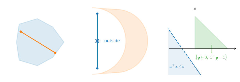
A quick non-example calibrates the definition. The annulus \(\{\mathbf{x} : 1 \le \|\mathbf{x}\| \le 2\}\) contains \((\pm \tfrac32, 0)\), but their midpoint is the origin, which the annulus excludes. This midpoint violates Equation 26.3.1.
26.3.1.2 Common Convex Sets in Machine Learning
Four common families of convex sets appear throughout this book.
- Hyperplanes and half-spaces. For the hyperplane \(\{\mathbf{x} : \mathbf{a}^\top\mathbf{x} = b\}\) and the half-space \(\{\mathbf{x} : \mathbf{a}^\top\mathbf{x} \le b\}\), the check is linearity: \(\mathbf{a}^\top(\theta\mathbf{x} + (1-\theta)\mathbf{y}) = \theta\, \mathbf{a}^\top\mathbf{x} + (1-\theta)\, \mathbf{a}^\top\mathbf{y}\), and an average of two numbers equal to \(b\) (or at most \(b\)) is again equal to \(b\) (or at most \(b\)).
- Norm balls. For any norm, \(\{\mathbf{x} : \|\mathbf{x}\| \le r\}\) is convex by the triangle inequality plus homogeneity: \(\|\theta\mathbf{x} + (1-\theta)\mathbf{y}\| \le \theta\|\mathbf{x}\| + (1-\theta)\|\mathbf{y}\| \le r\). This covers the \(\ell_2\) balls of weight decay and gradient clipping and the \(\ell_1\) balls of sparsity-inducing regularization alike.
- The probability simplex. \(\Delta = \{\mathbf{p} : \mathbf{p} \succeq 0,\ \mathbf{1}^\top\mathbf{p} = 1\}\), which contains attention weights, class probabilities, and mixture weights.
- The positive semidefinite cone. \(\mathbb{S}^n_+ = \{A = A^\top : \mathbf{z}^\top A \mathbf{z} \ge 0 \textrm{ for all } \mathbf{z}\}\), which contains covariance matrices and the Hessians certified below.
A notational convention, used throughout this part: the symbol \(\succeq\) (and its mirror \(\preceq\)) carries two senses, elementwise for vectors, as in \(\mathbf{p} \succeq 0\) above, and the semidefinite order for symmetric matrices, as in \(A \succeq 0\); the type of the operands says which is meant.
The final two families follow from closure under intersections.
26.3.1.3 New Convex Sets from Old
Proposition (intersections preserve convexity). Let \(\{C_i\}_{i \in I}\) be any family of convex sets, finite or infinite. Then \(C = \bigcap_{i \in I} C_i\) is convex.
Proof. Take \(\mathbf{x}, \mathbf{y} \in C\) and \(\theta \in [0, 1]\). For every \(i\), both points lie in the convex set \(C_i\), so \(\theta\mathbf{x} + (1-\theta)\mathbf{y} \in C_i\). A point in every \(C_i\) is a point in their intersection. \(\blacksquare\)
Unions have no such guarantee: \([0,1] \cup [2,3]\) is a union of two convex intervals whose chord from \(1\) to \(2\) leaves the set. Intersections preserve convexity; unions need not.
The proposition certifies most of the catalog. The probability simplex is the intersection of one hyperplane (\(\mathbf{1}^\top\mathbf{p} = 1\)) with \(n\) half-spaces (\(-p_i \le 0\)), hence convex and is therefore convex. The PSD cone is the intersection of infinitely many half-spaces, one per test vector: for each fixed \(\mathbf{z}\), the condition \(\mathbf{z}^\top A \mathbf{z} \ge 0\) is linear in the entries of \(A\), so \(\mathbb{S}^n_+ = \bigcap_{\mathbf{z}} \{A : \mathbf{z}^\top A \mathbf{z} \ge 0\}\) is convex, a fact used below for Hessians. More generally, every polyhedron \(\{\mathbf{x} : A\mathbf{x} \preceq \mathbf{b}\}\) is a finite intersection of half-spaces, and such polyhedra are the feasible sets of the constrained problems in Section 26.4.
Two additional constructions are useful. Affine maps preserve convexity in both directions: images and preimages of convex sets under \(\mathbf{x} \mapsto A\mathbf{x} + \mathbf{b}\) are convex, because affine maps send segments to segments. And any point cloud \(S\) generates a smallest convex superset, its convex hull: the intersection of every convex set containing \(S\) (convex by the proposition), or concretely the set of all weighted averages \(\sum_i \theta_i \mathbf{x}_i\) with \(\theta_i \ge 0\), \(\sum_i \theta_i = 1\). The two descriptions coincide: the set of weighted averages is itself convex and contains \(S\), so it contains the intersection, and the reverse inclusion (every convex superset contains all weighted averages) is Exercise 4’s induction. The simplex is the convex hull of the coordinate vectors: every probability distribution is an average of certainties.
26.3.2 Three Characterizations of Convex Functions
26.3.2.1 The Definition by Chords
A function \(f : C \to \mathbb{R}\) on a convex domain \(C\) is convex if its graph lies on or below every chord:
\[ f\left(\theta \mathbf{x} + (1 - \theta)\, \mathbf{y}\right) \;\le\; \theta f(\mathbf{x}) + (1 - \theta) f(\mathbf{y}) \qquad \textrm{for all } \mathbf{x}, \mathbf{y} \in C,\ \theta \in [0, 1]. \tag{26.3.2}\]
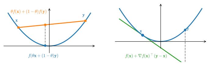
The left side evaluates \(f\) at a point of the segment; the right side is the height of the chord joining \((\mathbf{x}, f(\mathbf{x}))\) to \((\mathbf{y}, f(\mathbf{y}))\) above that same point. If the inequality is strict whenever \(\mathbf{x} \neq \mathbf{y}\) and \(\theta \in (0, 1)\), \(f\) is strictly convex; if \(-f\) is convex, \(f\) is concave. Note that the domain must be convex for the definition to even parse: the point \(\theta\mathbf{x} + (1-\theta)\mathbf{y}\) has to be somewhere \(f\) is defined.
Immediate consequence (local minima are global). If \(f\) is convex on a convex set \(C\), every local minimum is global. Let \(\mathbf{x}^\star\) be locally minimal and take any \(\mathbf{y}\in C\). For sufficiently small \(\theta>0\), the point \(\mathbf{z}_\theta=(1-\theta)\mathbf{x}^\star+\theta\mathbf{y}\) lies in the local neighborhood. Hence
\[ f(\mathbf{x}^\star)\le f(\mathbf{z}_\theta) \le (1-\theta)f(\mathbf{x}^\star)+\theta f(\mathbf{y}), \]
and rearranging gives \(f(\mathbf{x}^\star)\le f(\mathbf{y})\). Convexity thus turns a local optimality certificate into a global one. It does not, by itself, guarantee that a particular optimization algorithm reaches a minimizer.
Sets and functions are one theory: \(f\) is convex exactly when its epigraph \(\{(\mathbf{x}, t) : t \ge f(\mathbf{x})\}\), the region on and above the graph, is a convex set. Chords between points of the epigraph stay above the graph precisely when Equation 26.3.2 holds. This dictionary lets every fact about convex sets generate a fact about convex functions, and we will use it shortly.
26.3.2.2 The First-Order Condition
The chord condition requires no derivatives. When \(f\) is differentiable, an equivalent first-order test uses a tangent inequality: the first-order Taylor approximation at any point is a global under-estimator,
\[ f(\mathbf{y}) \;\ge\; f(\mathbf{x}) + \nabla f(\mathbf{x})^\top (\mathbf{y} - \mathbf{x}) \qquad \textrm{for all } \mathbf{x}, \mathbf{y} \in C. \tag{26.3.3}\]
The two equivalent conditions are shown in Figure 26.3.2. The chord condition is the definition: the chord joining any two points on the graph lies above the graph. The first-order condition uses the slope: the tangent at any point lies below the graph. This is the property gradient methods exploit: a single gradient evaluation at \(\mathbf{x}\) provides a lower bound valid at every other point in the domain. In particular, if \(\nabla f(\mathbf{x}) = \mathbf{0}\), then Equation 26.3.3 says \(f(\mathbf{y}) \ge f(\mathbf{x})\) for all \(\mathbf{y}\): a stationary point of a convex function is already a global minimum. We return to this in Section 26.3.4.
26.3.2.3 The Second-Order Condition
When \(f\) is twice differentiable on an open convex domain there is a third test, usually the easiest to run: \(f\) is convex if and only if its Hessian is positive semidefinite everywhere. On a lower-dimensional or closed domain, the test applies on the relative interior with the appropriate continuity at the boundary,
\[ \nabla^2 f(\mathbf{x}) \succeq 0 \qquad \textrm{for all } \mathbf{x} \in C. \]
In one dimension this is the calculus-class criterion \(f''(x) \ge 0\): the graph curves upward. In \(n\) dimensions it says every one-dimensional slice curves upward, since \(\mathbf{v}^\top \nabla^2 f(\mathbf{x})\, \mathbf{v}\) is the second derivative of \(f\) along the line through \(\mathbf{x}\) in direction \(\mathbf{v}\) (Section 25.2). Three applications follow. the quadratic \(\tfrac12\mathbf{x}^\top A \mathbf{x} + \mathbf{b}^\top\mathbf{x}\) (with \(A\) symmetric) has constant Hessian \(A\), so it is convex iff \(A \succeq 0\); the least-squares loss \(\tfrac12\|X\mathbf{w} - \mathbf{y}\|^2\) has Hessian \(X^\top X\), a Gram matrix, always PSD (Section 24.2.3.2); and \(e^x\), \(-\log x\), and \(x \log x\) are convex on their domains because their second derivatives \(e^x\), \(1/x^2\), and \(1/x\) are positive.
Proposition (the three characterizations agree). Let \(f\) be differentiable on an open convex domain \(C\). Then the chord condition Equation 26.3.2 and the first-order condition Equation 26.3.3 are equivalent. If \(f\) is twice differentiable, both are equivalent to \(\nabla^2 f(\mathbf{x}) \succeq 0\) on \(C\).
Proof. (Chord \(\Rightarrow\) first-order.) Fix \(\mathbf{x}, \mathbf{y}\) and \(\theta \in (0, 1]\). Rewriting Equation 26.3.2 at the point \(\mathbf{x} + \theta(\mathbf{y} - \mathbf{x})\) and subtracting \(f(\mathbf{x})\),
\[ \frac{f(\mathbf{x} + \theta(\mathbf{y} - \mathbf{x})) - f(\mathbf{x})}{\theta} \;\le\; f(\mathbf{y}) - f(\mathbf{x}). \]
As \(\theta \downarrow 0\) the left side converges to the directional derivative \(\nabla f(\mathbf{x})^\top(\mathbf{y} - \mathbf{x})\), giving Equation 26.3.3.
(First-order \(\Rightarrow\) chord.) Let \(\mathbf{z} = \theta\mathbf{x} + (1-\theta)\mathbf{y}\) and apply the under-estimator at \(\mathbf{z}\) twice, once toward each endpoint:
\[ f(\mathbf{x}) \ge f(\mathbf{z}) + \nabla f(\mathbf{z})^\top(\mathbf{x} - \mathbf{z}), \qquad f(\mathbf{y}) \ge f(\mathbf{z}) + \nabla f(\mathbf{z})^\top(\mathbf{y} - \mathbf{z}). \]
Multiply by \(\theta\) and \(1 - \theta\) and add: the gradient terms combine to \(\nabla f(\mathbf{z})^\top(\theta\mathbf{x} + (1-\theta)\mathbf{y} - \mathbf{z}) = 0\), leaving exactly Equation 26.3.2.
(Second-order \(\Rightarrow\) first-order.) Restrict to the segment: \(g(t) = f(\mathbf{x} + t(\mathbf{y} - \mathbf{x}))\) has \(g''(t) = (\mathbf{y} - \mathbf{x})^\top \nabla^2 f(\mathbf{x} + t(\mathbf{y} - \mathbf{x}))\,(\mathbf{y} - \mathbf{x}) \ge 0\). Taylor’s theorem with the Lagrange remainder (Section 25.1) gives \(g(1) = g(0) + g'(0) + \tfrac12 g''(\tau)\) for some \(\tau \in (0, 1)\), and dropping the nonnegative remainder is Equation 26.3.3.
(First-order \(\Rightarrow\) second-order.) Suppose instead \(\mathbf{v}^\top \nabla^2 f(\mathbf{x})\, \mathbf{v} < 0\) for some \(\mathbf{x}\) and \(\mathbf{v}\). Expanding along that direction,
\[ f(\mathbf{x} + t\mathbf{v}) = f(\mathbf{x}) + t\, \nabla f(\mathbf{x})^\top\mathbf{v} + \frac{t^2}{2}\, \mathbf{v}^\top \nabla^2 f(\mathbf{x})\, \mathbf{v} + o(t^2), \]
so for small enough \(t > 0\) the left side drops strictly below the tangent value \(f(\mathbf{x}) + t \nabla f(\mathbf{x})^\top\mathbf{v}\), contradicting Equation 26.3.3. \(\blacksquare\)
The appropriate characterization depends on the available structure. The chord condition needs no smoothness (it certifies \(\|\mathbf{x}\|_1\) and the hinge loss, where Hessians do not exist); the first-order condition is used in optimization proofs; the second-order condition is the usual test for smooth losses, where checking convexity means checking a matrix is PSD, the territory of Section 24.2.
26.3.2.4 Strong Convexity
Convexity bounds curvature from below by zero. Two refinements sharpen the geometry. \(f\) is strictly convex if the chord inequality is strict, ruling out flat segments. More quantitatively, \(f\) is \(\mu\)-strongly convex (for \(\mu > 0\)) if \(f(\mathbf{x}) - \tfrac{\mu}{2}\|\mathbf{x}\|^2\) is convex, or equivalently, by the first-order condition,
\[ f(\mathbf{y}) \;\ge\; f(\mathbf{x}) + \nabla f(\mathbf{x})^\top(\mathbf{y} - \mathbf{x}) + \frac{\mu}{2}\, \|\mathbf{y} - \mathbf{x}\|^2, \tag{26.3.4}\]
or, by the second-order condition, \(\nabla^2 f \succeq \mu I\) everywhere. Strong convexity requires a quadratic lower bound relative to every tangent, with a positive minimum curvature. Paired with the \(L\)-smoothness of Section 26.1 (\(\nabla^2 f \preceq L I\)), the function has quadratic lower and upper bounds, and the ratio \(\kappa = L/\mu\) is precisely the condition number that governed convergence speed there. A useful source of strong convexity: adding the ridge penalty \(\tfrac{\lambda}{2}\|\mathbf{w}\|^2\) to any convex loss makes the sum \(\lambda\)-strongly convex, which is another effect of weight decay.
26.3.2.5 The Subgradient
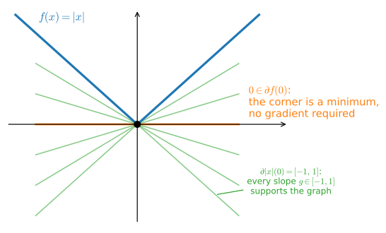
The losses \(\|\mathbf{x}\|_1\) and \(\max(0, 1 - z)\) have corners, so Equation 26.3.3 cannot be checked as written: there is no gradient at the kink. Section 25.1 already repaired this in one dimension with the subgradient Equation 25.1.8, computed \(\partial |x|(0) = [-1, 1]\) there, and proved the optimality test \(0 \in \partial f(x^\star)\) (Equation 25.1.9). The vector form is the same idea: a vector \(\mathbf{g}\) is a subgradient of \(f\) at \(\mathbf{x}\) if it provides the same global under-estimate a gradient would:
\[ f(\mathbf{y}) \;\ge\; f(\mathbf{x}) + \mathbf{g}^\top (\mathbf{y} - \mathbf{x}) \qquad \textrm{for all } \mathbf{y}, \tag{26.3.5}\]
and the set of all subgradients at \(\mathbf{x}\) is written \(\partial f(\mathbf{x})\). Where \(f\) is differentiable it collapses to the singleton \(\{\nabla f(\mathbf{x})\}\); at a corner it can contain multiple vectors (Figure 26.3.3), as it did for \(|x|\) and as it does for the hinge \(\max(0, 1 - z)\) at \(z = 1\), where \(\partial f(1) = [-1, 0]\). The same optimality criterion applies: \(\mathbf{x}^\star\) minimizes \(f\) iff \(\mathbf{0} \in \partial f(\mathbf{x}^\star)\). The following existence result is used without proof:
Supporting-hyperplane fact. A convex \(f\) has at least one subgradient at every interior point of its domain; geometrically, a supporting line (a supporting hyperplane, in \(n\) dimensions) fits under the graph. See (Rockafellar 1970) (or Boyd and Vandenberghe (2004), section 2.5).
Subgradients preserve the supporting-hyperplane, Jensen, and local-equals-global arguments at ReLU-style kinks. Optimization algorithms need their own analysis: a subgradient step need not decrease the objective, and the standard subgradient method uses diminishing steps and has slower rates than smooth gradient descent.
26.3.2.6 Checking the Characterizations Numerically
The three characterizations identify the same convex functions; the code checks all three on the least-squares loss \(f(\mathbf{w}) = \tfrac12\|X\mathbf{w} - \mathbf{y}\|^2\) in two weights: random chords, random tangents, and the eigenvalues of the Hessian.
rng = np.random.default_rng(0)
X = rng.normal(size=(20, 2))                   # design matrix, 20 points
y = rng.normal(size=20)
f = lambda w: 0.5 * ((X @ w - y) ** 2).sum()
grad = lambda w: X.T @ (X @ w - y)
worst_chord, worst_tangent = -np.inf, -np.inf
for _ in range(1000):
    u, v = rng.normal(size=(2, 2)) * 3.0       # random pair of weight vectors
    t = rng.uniform()
    worst_chord = max(worst_chord,             # f(chord point) - chord height
                      f(t * u + (1 - t) * v) - (t * f(u) + (1 - t) * f(v)))
    worst_tangent = max(worst_tangent,         # tangent value - f
                        f(u) + grad(u) @ (v - u) - f(v))
print(f'worst chord violation over 1000 trials:   {worst_chord:.2e}')
print(f'worst tangent violation over 1000 trials: {worst_tangent:.2e}')
print('Hessian eigenvalues:', np.linalg.eigvalsh(X.T @ X).round(4))
worst chord violation over 1000 trials: -2.46e-03
worst tangent violation over 1000 trials: -4.95e-02
Hessian eigenvalues: [ 6.273 18.6557]All three checks agree. The worst chord “violation” across a thousand random trials is \(-2.46 \times 10^{-3}\) and the worst tangent violation is \(-4.95 \times 10^{-2}\), both negative, meaning every sampled chord and tangent inequality holds; and the Hessian’s eigenvalues, \(6.273\) and \(18.6557\), are positive. (Sampling can only ever refute convexity, never prove it; the Hessian check is the one that constitutes a proof, since \(X^\top X\) is the same matrix at every \(\mathbf{w}\).)
26.3.3 Jensen’s Inequality
The chord definition compares \(f\) at a two-point average against the average of \(f\) at the two points. Nothing about the argument is special to two: applying Equation 26.3.2 repeatedly (Exercise 4) gives the finite form
\[ f\left(\sum_i \theta_i \mathbf{x}_i\right) \;\le\; \sum_i \theta_i\, f(\mathbf{x}_i), \qquad \theta_i \ge 0,\ \sum_i \theta_i = 1, \]
and a set of nonnegative weights summing to one is exactly a probability distribution. The full generalization replaces averages by expectations; the probabilistic chapters of this book use it constantly.
Proposition (Jensen’s inequality). Let \(f\) be convex and let \(X\) be a random vector taking values in \(f\)’s domain, with \(\mathbb{E}[X]\) finite and in the domain’s interior, and read \(\mathbb{E}[f(X)]\) as an extended real number (the value \(+\infty\) is allowed, and makes the inequality trivially true). Then
\[ f\left(\mathbb{E}[X]\right) \;\le\; \mathbb{E}\left[f(X)\right]. \tag{26.3.6}\]
If \(f\) is strictly convex, equality holds if and only if \(X = \mathbb{E}[X]\) almost surely.
Proof. Let \(\boldsymbol{\mu} = \mathbb{E}[X]\) and pick a subgradient \(\mathbf{g} \in \partial f(\boldsymbol{\mu})\); the granted fact (supporting hyperplane) provides one at an interior point. The supporting-line inequality Equation 26.3.5 holds pointwise for every outcome:
\[ f(X) \;\ge\; f(\boldsymbol{\mu}) + \mathbf{g}^\top (X - \boldsymbol{\mu}). \]
Take expectations of both sides: the linear term has mean zero, leaving \(\mathbb{E}[f(X)] \ge f(\boldsymbol{\mu})\). For strictly convex \(f\) the supporting line touches the graph only at \(\boldsymbol{\mu}\): if it also touched at some \(\mathbf{x} \neq \boldsymbol{\mu}\), strict convexity at the midpoint would force \(f\bigl(\tfrac{\mathbf{x} + \boldsymbol{\mu}}{2}\bigr) < \tfrac12 f(\mathbf{x}) + \tfrac12 f(\boldsymbol{\mu})\), which equals the (affine) supporting line’s value there, contradicting that the line under-estimates \(f\) everywhere. So the pointwise inequality is strict on the event \(X \neq \boldsymbol{\mu}\); equality in expectation therefore forces that event to have probability zero. \(\blacksquare\)
The proof uses the first-order condition (in subgradient form, so no smoothness is needed) plus linearity of expectation. For a convex function, dispersing \(X\) can increase the average value \(f(X)\). For concave \(f\) the inequality flips: \(\mathbb{E}[f(X)] \le f(\mathbb{E}[X])\).
An immediate corollary is the nonnegativity of KL divergence. Section 28.1 restates it as Gibbs’ inequality and derives the entropy upper bound \(H(X) \le \log k\) and the nonnegativity of mutual information on it; that section is also the KL divergence’s definitional home, with its \(0 \log 0\) and support conventions.
Corollary (nonnegativity of KL divergence). For probability distributions \(p\) and \(q\) on a common finite alphabet (with \(q(x) > 0\) where \(p(x) > 0\)),
\[ D_{\mathrm{KL}}(p \,\|\, q) \;=\; \sum_x p(x) \log \frac{p(x)}{q(x)} \;\ge\; 0, \]
with equality if and only if \(p = q\).
Proof. Apply Jensen’s inequality to the strictly convex function \(-\log\) and the random variable \(R = q(X)/p(X)\) with \(X \sim p\):
\[ D_{\mathrm{KL}}(p \,\|\, q) = \mathbb{E}_p\left[-\log R\right] \;\ge\; -\log \mathbb{E}_p[R] = -\log \sum_{x : p(x) > 0} p(x)\, \frac{q(x)}{p(x)} \;\ge\; -\log 1 = 0, \]
since \(\sum_{x : p(x) > 0} q(x) \le 1\). By the equality case, the bound is tight iff \(R\) is almost surely constant and the \(q\)-mass off \(p\)’s support is zero, i.e., \(q = c\,p\) with \(c = 1\): \(p = q\). \(\blacksquare\)
The same one-liner with the concave \(\log\) yields the classical arithmetic–geometric mean inequality: for positive \(x_1, \ldots, x_n\), concavity gives \(\log\bigl(\tfrac1n \sum_i x_i\bigr) \ge \tfrac1n \sum_i \log x_i\), and exponentiating,
\[ \frac{1}{n} \sum_{i=1}^n x_i \;\ge\; \left(\prod_{i=1}^n x_i\right)^{1/n}, \]
with equality iff all \(x_i\) coincide (\(\log\) is strictly concave). Jensen also explains a previously encountered gap: the evidence lower bound of Section 27.3.5 is Jensen applied to the concave \(\log\) of an expectation, and the slack in the ELBO is the Jensen gap. The following cell evaluates the inequality in three ways: a Monte Carlo estimate of \(\mathbb{E}[e^X]\) versus \(e^{\mathbb{E}[X]}\), a bulk test of AM–GM, and the KL corollary on a thousand random distribution pairs.
rng = np.random.default_rng(1)
z = rng.normal(size=1_000_000)                 # X ~ N(0, 1)
print(f'E[exp(X)] = {np.exp(z).mean():.4f}  vs  exp(E[X]) = {np.exp(z.mean()):.4f}'
      f'  (theory: sqrt(e) = {np.exp(0.5):.4f} vs 1)')
u = rng.uniform(0.1, 10.0, size=(100_000, 5))  # AM-GM from concavity of log
am, gm = u.mean(axis=1), np.exp(np.log(u).mean(axis=1))
print(f'AM >= GM in all trials: {bool((am >= gm).all())},'
      f'  smallest AM/GM ratio = {(am / gm).min():.4f}')
p = rng.dirichlet(np.ones(10), size=1000)      # 1000 random distribution pairs
q = rng.dirichlet(np.ones(10), size=1000)
print(f'min KL(p||q) = {(p * np.log(p / q)).sum(axis=1).min():.4f} >= 0,'
      f'  max |KL(p||p)| = {np.abs((p * np.log(p / p)).sum(axis=1)).max():.1e}')
E[exp(X)] = 1.6466 vs exp(E[X]) = 0.9998 (theory: sqrt(e) = 1.6487 vs 1)
AM >= GM in all trials: True, smallest AM/GM ratio = 1.0002
min KL(p||q) = 0.1331 >= 0, max |KL(p||p)| = 0.0e+00With \(X \sim \mathcal{N}(0, 1)\) and the convex \(f(x) = e^x\), a million samples give \(\mathbb{E}[e^X] \approx 1.6466\) against \(e^{\mathbb{E}[X]} \approx 0.9998\); the true values are \(\sqrt{e} \approx 1.6487\) and \(1\), a Jensen gap of \(0.65\). Additional sampling reduces estimation error but not this population gap. AM \(\ge\) GM holds in all \(10^5\) random draws (smallest ratio \(1.0002\)), and across a thousand random pairs of distributions on ten symbols the smallest KL divergence is \(0.1331\), comfortably nonnegative, while \(D_{\mathrm{KL}}(p\,\|\,p)\) prints as 0.0e+00: the equality case, exact at machine resolution.
26.3.4 Why Convexity Matters
26.3.4.1 Geometry, Minimizers, and Uniqueness
The local-to-global proposition following the definition is the main optimization consequence of convexity. Figure 26.3.4 contrasts the illustrated smooth convex objective with a nonconvex objective having two basins. For the displayed step size and starting points, gradient descent reaches the convex minimizer in the first panel but can reach different local minima in the second. This algorithmic behavior also depends on smoothness and a stable step size.
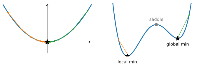
The same chord argument shows that the minimizer set is convex: if \(\mathbf{x}\) and \(\mathbf{y}\) both attain \(f^\star\), every point between them does as well. For differentiable \(f\) on an open domain, the first-order condition also shows that \(\nabla f(\mathbf{x})=0\) implies global optimality. A stronger assumption gives uniqueness.
Proposition (uniqueness). A strictly convex \(f\) has at most one minimizer; a continuous, strongly convex \(f\) on a closed convex set has exactly one.
Proof. If \(\mathbf{x} \neq \mathbf{y}\) were both minimizers with value \(f^\star\), the strict chord inequality at \(\theta = \tfrac12\) would give \(f\bigl(\tfrac{\mathbf{x} + \mathbf{y}}{2}\bigr) < f^\star\), a contradiction. Strong convexity adds existence. Write \(f = h + \tfrac{\mu}{2}\|\cdot\|^2\) with \(h\) convex, fix an interior point \(\mathbf{x}_0\) and a subgradient \(\mathbf{g} \in \partial h(\mathbf{x}_0)\) (the granted fact supplies one), and add the quadratic back: expanding \(\|\mathbf{y}\|^2 = \|\mathbf{x}_0\|^2 + 2\mathbf{x}_0^\top(\mathbf{y} - \mathbf{x}_0) + \|\mathbf{y} - \mathbf{x}_0\|^2\) turns \(h(\mathbf{y}) \ge h(\mathbf{x}_0) + \mathbf{g}^\top(\mathbf{y} - \mathbf{x}_0)\) into
\[ f(\mathbf{y}) \;\ge\; f(\mathbf{x}_0) + (\mathbf{g} + \mu\mathbf{x}_0)^\top (\mathbf{y} - \mathbf{x}_0) + \frac{\mu}{2}\, \|\mathbf{y} - \mathbf{x}_0\|^2, \]
the subgradient form of Equation 26.3.4, valid with no differentiability assumed. So \(f\) grows at least quadratically away from \(\mathbf{x}_0\) and its sublevel sets are bounded; a continuous function on a closed bounded set attains its minimum. \(\blacksquare\)
The continuity hypothesis is automatic in the interior, where convex functions are always continuous; it matters only at the boundary of the closed set, where a convex function may jump upward and the minimum can fail to be attained.
The following experiment compares convex and nonconvex objectives using the same gradient-descent loop, the same step size, the same \(500\) random starting points, on a convex bowl \(f(x) = (x - \tfrac12)^2\) and on the tilted double well \(g(x) = (x^2 - 1)^2 + x/2\).
def gd(grad_fn, x, eta=0.05, steps=600):
    for _ in range(steps):
        x = x - eta * grad_fn(x)
    return x

rng = np.random.default_rng(2)
inits = rng.uniform(-1.5, 1.5, size=500)       # 500 random starting points
bowl = gd(lambda x: 2 * (x - 0.5), inits)      # convex: f(x) = (x - 1/2)^2
g = lambda x: (x**2 - 1)**2 + 0.5 * x          # non-convex: tilted double well
well = gd(lambda x: 4 * x * (x**2 - 1) + 0.5, inits)
left, right = well[well < 0], well[well > 0]
print(f'convex bowl: all {bowl.size} runs end at x = {bowl.mean():.6f}'
      f'  (spread {np.ptp(bowl):.1e})')
print(f'double well: {left.size} runs -> x = {left.mean():.4f}'
      f'  (g = {g(left.mean()):.4f})')
print(f'             {right.size} runs -> x = {right.mean():.4f}'
      f'  (g = {g(right.mean()):.4f})')
convex bowl: all 500 runs end at x = 0.500000 (spread 6.7e-16)
double well: 271 runs -> x = -1.0575 (g = -0.5148)
229 runs -> x = 0.9304 (g = 0.4833)On the convex quadratic, all \(500\) runs converge to \(x = 0.5\) with a spread of \(6.7 \times 10^{-16}\), machine epsilon; the histogram of outcomes is a single spike. On the double well the histogram has two bars: \(271\) runs find the global minimum at \(x \approx -1.06\) with \(g \approx -0.515\), while the other \(229\) converge to the local minimum at \(x \approx 0.93\) with \(g \approx 0.483\), nearly a full unit worse, and further descent remains at that local minimum. The algorithm was identical in the two lines; the difference arises from the objectives under this stable step size. Convexity rules out nonglobal local minima, while convergence still depends on smoothness and the step size.
26.3.4.2 From Local Steps to Global Rates
Section 26.1 proved the descent lemma Equation 26.1.5: for \(L\)-smooth \(f\), the gradient step \(\mathbf{x}_{t+1} = \mathbf{x}_t - \tfrac{1}{L} \nabla f(\mathbf{x}_t)\) achieves \(f(\mathbf{x}_{t+1}) \le f(\mathbf{x}_t) - \tfrac{1}{2L} \|\nabla f(\mathbf{x}_t)\|^2\). By itself this guarantees only that gradients eventually vanish, a stationary point, which in general may be a saddle or a poor local minimum. Convexity upgrades the stationarity guarantee to a quantitative global optimality guarantee. The next two propositions state these rates (Nesterov 2018).
Proposition (gradient descent on smooth convex functions). Let \(f\) be convex and \(L\)-smooth with a minimizer \(\mathbf{x}^\star\). Gradient descent with \(\eta = 1/L\) satisfies, for every \(k \ge 1\),
\[ f(\mathbf{x}_k) - f(\mathbf{x}^\star) \;\le\; \frac{L\, \|\mathbf{x}_0 - \mathbf{x}^\star\|^2}{2k}. \tag{26.3.7}\]
Proof. Chain the descent lemma into the first-order lens Equation 26.3.3 aimed at the optimum, \(f(\mathbf{x}_t) - f(\mathbf{x}^\star) \le \nabla f(\mathbf{x}_t)^\top(\mathbf{x}_t - \mathbf{x}^\star)\):
\[ f(\mathbf{x}_{t+1}) - f(\mathbf{x}^\star) \;\le\; \nabla f(\mathbf{x}_t)^\top (\mathbf{x}_t - \mathbf{x}^\star) - \frac{1}{2L} \|\nabla f(\mathbf{x}_t)\|^2. \]
Completing the square turns the right side into a difference of distances:
\[ \nabla f(\mathbf{x}_t)^\top (\mathbf{x}_t - \mathbf{x}^\star) - \frac{1}{2L} \|\nabla f(\mathbf{x}_t)\|^2 = \frac{L}{2} \left( \|\mathbf{x}_t - \mathbf{x}^\star\|^2 - \left\|\mathbf{x}_t - \mathbf{x}^\star - \tfrac{1}{L}\nabla f(\mathbf{x}_t)\right\|^2 \right), \]
and the second norm is exactly \(\|\mathbf{x}_{t+1} - \mathbf{x}^\star\|^2\). Summing over \(t = 0, \ldots, k-1\), the right side telescopes:
\[ \sum_{t=0}^{k-1} \left( f(\mathbf{x}_{t+1}) - f(\mathbf{x}^\star) \right) \;\le\; \frac{L}{2} \left( \|\mathbf{x}_0 - \mathbf{x}^\star\|^2 - \|\mathbf{x}_k - \mathbf{x}^\star\|^2 \right) \;\le\; \frac{L}{2}\, \|\mathbf{x}_0 - \mathbf{x}^\star\|^2. \]
The descent lemma makes \(f(\mathbf{x}_t)\) nonincreasing, so the last term of the sum is the smallest: \(k \left(f(\mathbf{x}_k) - f(\mathbf{x}^\star)\right)\) is at most the sum, which gives Equation 26.3.7. \(\blacksquare\)
Two remarks. The bound is dimension-free: the displayed iteration bound has no explicit dependence on parameter count. Dimension can still affect curvature constants and per-iteration cost. The telescoping display also implies that every bracket is nonnegative (its left factor is \(f(\mathbf{x}_{t+1}) - f^\star \ge 0\)), so \(\|\mathbf{x}_t - \mathbf{x}^\star\|\) never increases: the iterates move monotonically closer to the optimum.
With strong convexity, the sublinear \(O(1/k)\) sharpens to a geometric decay.
Proposition (linear rate under strong convexity). Let \(f\) be \(\mu\)-strongly convex and \(L\)-smooth, with minimizer \(\mathbf{x}^\star\). Gradient descent with \(\eta = 1/L\) satisfies
\[ f(\mathbf{x}_k) - f(\mathbf{x}^\star) \;\le\; \left(1 - \frac{\mu}{L}\right)^{k} \left( f(\mathbf{x}_0) - f(\mathbf{x}^\star) \right). \tag{26.3.8}\]
Proof. First, strong convexity links the gradient’s size to the remaining suboptimality. Minimize both sides of Equation 26.3.4 over \(\mathbf{y}\): the left side’s infimum is \(f(\mathbf{x}^\star)\), and the right side is a quadratic in \(\mathbf{y}\) minimized at \(\mathbf{y} = \mathbf{x} - \tfrac{1}{\mu}\nabla f(\mathbf{x})\), where it equals \(f(\mathbf{x}) - \tfrac{1}{2\mu}\|\nabla f(\mathbf{x})\|^2\). Hence
\[ \frac12\, \|\nabla f(\mathbf{x})\|^2 \;\ge\; \mu \left( f(\mathbf{x}) - f(\mathbf{x}^\star) \right) \qquad \textrm{for all } \mathbf{x}. \tag{26.3.9}\]
Substitute Equation 26.3.9 into the descent lemma:
\[ f(\mathbf{x}_{t+1}) - f(\mathbf{x}^\star) \;\le\; f(\mathbf{x}_t) - f(\mathbf{x}^\star) - \frac{1}{2L} \|\nabla f(\mathbf{x}_t)\|^2 \;\le\; \left(1 - \frac{\mu}{L}\right) \left( f(\mathbf{x}_t) - f(\mathbf{x}^\star) \right), \]
and iterate \(k\) times. \(\blacksquare\)
The contraction factor is \(1 - 1/\kappa\) with \(\kappa = L/\mu\) the condition number: reaching accuracy \(\epsilon\) costs \(O(\kappa \log(1/\epsilon))\) iterations, against \(O(1/\epsilon)\) without strong convexity. This is the global, every-start version of the per-mode contraction that Section 26.1 measured on quadratics. One observation will be used later: the second half of the proof never used convexity at all. It consumed only the inequality Equation 26.3.9, a fact that yields a rate under the PL condition without convexity.
Both rates can be measured. The cell runs gradient descent at \(\eta = 1/L\) on the least-squares toy of the #convexity-three-lenses cell (strongly convex, with \(\mu\) and \(L\) read off the eigenvalues of \(X^\top X\)) and prints the per-step contraction of \(f - f^\star\) next to the theorem’s bound:
mu, L = np.linalg.eigvalsh(X.T @ X)[[0, -1]]   # curvature floor and ceiling
w_star = np.linalg.solve(X.T @ X, X.T @ y)     # the unique minimizer
w, gaps = np.zeros(2), []
for _ in range(25):                            # gradient descent at eta = 1/L
    w -= grad(w) / L
    gaps.append(f(w) - f(w_star))
r = np.array(gaps[1:]) / np.array(gaps[:-1])
print(f'mu = {mu:.4f}, L = {L:.4f}:  the theorem promises '
      f'contraction <= 1 - mu/L = {1 - mu / L:.4f}')
print('measured per-step contraction of f - f*:', r[::6].round(4))
print(f'worst step: {r.max():.4f}  (the bound holds at every step)')
mu = 6.2730, L = 18.6557: the theorem promises contraction <= 1 - mu/L = 0.6637
measured per-step contraction of f - f*: [0.4406 0.4406 0.4406 0.4406]
worst step: 0.4406 (the bound holds at every step)The measured contraction is \(0.4406\) at every step, safely inside the promised \(1 - \mu/L = 0.6637\), and the gap between the two is itself informative. On a pure quadratic the slow mode’s distance to the optimum contracts by exactly \(1 - \mu/L\) per step, and the value gap, being quadratic in the distance, contracts by its square: \((1 - \mu/L)^2 = 0.4406\), precisely the printed figure. So the theorem’s bound is valid across the whole smooth strongly convex class, but on quadratics it is loose by exactly a square. A particular function can converge faster than this upper bound.
26.3.5 Recognizing Convexity and Its Limits
26.3.5.1 A Calculus of Convex Functions
Most convexity proofs in practice are assembled from parts rather than computed from Hessians: a small set of operations preserves convexity, and many losses are built from convex atoms by these operations.
- Nonnegative weighted sums. If \(f_1, \ldots, f_m\) are convex and \(w_i \ge 0\), then \(\sum_i w_i f_i\) is convex: multiply the chord inequality for each \(f_i\) by \(w_i\) and add. (An average of losses over a training set is a nonnegative weighted sum.)
- Affine pre-composition. If \(f\) is convex then so is \(\mathbf{x} \mapsto f(A\mathbf{x} + \mathbf{b})\): affine maps send the segment between \(\mathbf{x}\) and \(\mathbf{y}\) to the segment between their images, with the same \(\theta\), so the chord inequality transfers verbatim. (A loss that is convex in a model’s output is convex in the weights of a linear model producing that output.)
- Pointwise maximum and supremum. If each \(f_i\) is convex, so is \(\max_i f_i\), and the proof is the epigraph dictionary in action: the epigraph of a max is the intersection of the epigraphs, and intersections of convex sets are convex. The upper envelope of any family of lines is convex, however large the family.
- Monotone convex composition. If \(g\) is convex and \(h\) is convex and nondecreasing, then \(h(g(\mathbf{x}))\) is convex (in one dimension: \((h \circ g)'' = h''(g)\,(g')^2 + h'(g)\, g'' \ge 0\), each summand nonnegative). The monotonicity hypothesis is essential: \(h(t) = t^2\) and \(g(x) = x^2 - 1\) compose to the double-well example above create nonglobal local minima.
These rules certify most of the convex losses in this book directly. The hinge loss \(\max(0, 1 - y\,\mathbf{w}^\top\mathbf{x})\) is a maximum of two affine functions of \(\mathbf{w}\) (rules 3 and 2). The \(\ell_1\) norm \(\|\mathbf{w}\|_1 = \sum_i \max(w_i, -w_i)\) is a sum of maxima of affine functions (rules 1, 3, 2). The logistic loss \(\log(1 + e^{-y\,\mathbf{w}^\top\mathbf{x}})\) is the convex \(t \mapsto \log(1 + e^t)\) (second derivative \(\sigma'(t) = \sigma(t)(1-\sigma(t)) > 0\)) pre-composed with an affine map, then summed over data. Adding ridge regularization to a convex loss gives a sum of a convex and \(\lambda\)-strongly convex function, hence strongly convex (rule 1 applied to Equation 26.3.4). One operation is absent from the list: composition with nonlinear, non-monotone inner maps, and standard multilayer parameterizations do not satisfy this composition rule.
26.3.5.2 Log-Sum-Exp and the Softmax Covariance
A central example is the function behind every softmax cross-entropy loss. Define \(\mathrm{lse}(\mathbf{x}) = \log \sum_{i=1}^n e^{x_i}\), the smooth maximum of Section 26.5.
Proposition (log-sum-exp is convex). The Hessian of \(\mathrm{lse}\) at \(\mathbf{x}\) is
\[ \nabla^2 \mathrm{lse}(\mathbf{x}) = \mathrm{diag}(\mathbf{s}) - \mathbf{s}\mathbf{s}^\top, \qquad \mathbf{s} = \mathrm{softmax}(\mathbf{x}), \]
which is the covariance matrix of the one-hot encoding of a class drawn from \(\mathbf{s}\), hence PSD, hence \(\mathrm{lse}\) is convex.
Proof. Differentiating once gives \(\partial\, \mathrm{lse} / \partial x_i = e^{x_i} / \sum_j e^{x_j} = s_i\): the gradient of \(\mathrm{lse}\) is the softmax. Differentiating again gives the softmax Jacobian Equation 25.3.7, derived in Section 25.3, which is the claimed matrix. Now let \(I\) be a random index with \(\Pr(I = i) = s_i\) and let \(\mathbf{e}_I\) be its one-hot vector. Then \(\mathbb{E}[\mathbf{e}_I] = \mathbf{s}\) and \(\mathbb{E}[\mathbf{e}_I \mathbf{e}_I^\top] = \mathrm{diag}(\mathbf{s})\), so \(\mathrm{Cov}(\mathbf{e}_I) = \mathrm{diag}(\mathbf{s}) - \mathbf{s}\mathbf{s}^\top\) is exactly the Hessian. Covariances are PSD; directly,
\[ \mathbf{v}^\top \nabla^2 \mathrm{lse}\, \mathbf{v} = \sum_i s_i v_i^2 - \left(\sum_i s_i v_i\right)^2 = \mathbb{E}\left[v_I^2\right] - \left(\mathbb{E}[v_I]\right)^2 = \mathrm{Var}(v_I) \;\ge\; 0. \;\blacksquare \]
A direct corollary is the cross-entropy loss in the logits, \(\ell(\mathbf{z}) = \mathrm{lse}(\mathbf{z}) - z_y\) for true class \(y\), is log-sum-exp plus an affine function, hence convex. Softmax regression (Section 3.1) composes it with the affine map \(\mathbf{z} = W\mathbf{x} + \mathbf{b}\), so the loss is convex in the weights (rule 2): for fixed features, optimizing only the linear classifier weights is a convex problem. The same softmax machinery is also the core of attention: a head’s weights are exactly this map applied to scaled query–key scores (Section 10.2), with the same Jacobian \(\mathrm{diag}(\mathbf{s}) - \mathbf{s}\mathbf{s}^\top\) appearing in its backward pass. The Hessian formula also predicts one zero eigenvalue, in the direction \(\mathbf{1}\): a variance \(\mathrm{Var}(v_I)\) vanishes when \(v\) is constant, which is the shift invariance \(\mathrm{lse}(\mathbf{x} + c\mathbf{1}) = \mathrm{lse}(\mathbf{x}) + c\), the identity used by the numerically stable softmax of Section 26.5. The cell verifies these properties: the eigenvalues, the covariance identity by Monte Carlo, and the flat direction.
lse = lambda x: x.max() + np.log(np.exp(x - x.max()).sum())
rng = np.random.default_rng(3)
x = rng.normal(size=6)                         # six logits
s = np.exp(x - lse(x))                         # softmax(x)
H = np.diag(s) - np.outer(s, s)                # analytic Hessian of lse
print('eigenvalues of H:', np.linalg.eigvalsh(H).round(6))
draws = rng.choice(len(x), size=200_000, p=s)  # class I ~ Categorical(s)
onehot = np.eye(len(x))[draws]
print(f'max |H - covariance of one-hot samples| = '
      f'{np.abs(H - np.cov(onehot.T)).max():.4f}')
print(f'max |H @ 1| = {np.abs(H.sum(axis=1)).max():.1e}  (flat shift direction)')
eigenvalues of H: [-0. 0.008103 0.052497 0.063313 0.099101 0.284324]
max |H - covariance of one-hot samples| = 0.0006
max |H @ 1| = 1.8e-16 (flat shift direction)Every eigenvalue is nonnegative, from \(0.284324\) down to one numerical zero, the predicted flat direction, confirmed by \(\|H\mathbf{1}\|_\infty \approx 1.8 \times 10^{-16}\). And the empirical covariance of \(200{,}000\) one-hot draws matches the analytic Hessian to within \(0.0006\): the empirical covariance agrees with the analytic Hessian.
26.3.5.3 The Convex Conjugate
The convex conjugate connects this section with duality (Section 26.4) and the variational representations of information theory. From here on we allow \(f\) to take the value \(+\infty\); convexity for such an extended-real function is read on its epigraph (the chord inequality is required wherever the values are finite), and the conjugates below produce \(+\infty\) naturally. The convex conjugate (or Fenchel–Legendre transform) of \(f : \mathbb{R}^n \to \mathbb{R} \cup \{+\infty\}\) is
\[ f^*(\mathbf{y}) \;=\; \sup_{\mathbf{x}} \;\left( \mathbf{y}^\top \mathbf{x} - f(\mathbf{x}) \right). \tag{26.3.10}\]
Geometrically, \(f^*(\mathbf{y})\) asks: among all affine functions with slope \(\mathbf{y}\), what is the largest intercept compatible with remaining below the graph of \(f\)? (It records the negative of that intercept.) The conjugate thus encodes \(f\) by its supporting lines instead of its values, and for closed convex \(f\) (closed meaning the epigraph is a closed set, equivalently \(f\) is lower semicontinuous) the encoding is lossless: \(f^{**} = f\) (Boyd and Vandenberghe (2004), section 3.3). For non-convex \(f\) the double transform returns the largest closed convex function below it, the convex envelope, which is what convex relaxations optimize in place of \(f\).
Two properties are immediate. First, \(f^*\) is always convex, whatever \(f\) is: for fixed \(\mathbf{x}\) the expression \(\mathbf{y}^\top\mathbf{x} - f(\mathbf{x})\) is affine in \(\mathbf{y}\), and rule 3 says a supremum of affine functions is convex. The same one-line argument, in the next section, makes the dual function of Section 26.4.4 concave, and that is no coincidence: for linearly constrained problems the dual function can be written in terms of a conjugate. Second, the definition rearranges into the Fenchel–Young inequality,
\[ \mathbf{y}^\top \mathbf{x} \;\le\; f(\mathbf{x}) + f^*(\mathbf{y}) \qquad \textrm{for all } \mathbf{x}, \mathbf{y}, \tag{26.3.11}\]
with equality exactly when \(\mathbf{x}\) attains the supremum; for differentiable \(f\), when \(\mathbf{y} = \nabla f(\mathbf{x})\).
The simplest example sets the pattern: for \(f(\mathbf{x}) = \tfrac12\|\mathbf{x}\|^2\), the supremum of \(\mathbf{y}^\top\mathbf{x} - \tfrac12\|\mathbf{x}\|^2\) is attained at \(\mathbf{x} = \mathbf{y}\), giving \(f^*(\mathbf{y}) = \tfrac12\|\mathbf{y}\|^2\): the squared norm is its own conjugate, and Fenchel–Young becomes the familiar \(\mathbf{y}^\top\mathbf{x} \le \tfrac12\|\mathbf{x}\|^2 + \tfrac12\|\mathbf{y}\|^2\).
The pair that matters for deep learning is log-sum-exp \(\leftrightarrow\) negative entropy. Compute \(\mathrm{lse}^*(\mathbf{p}) = \sup_{\mathbf{x}} \mathbf{p}^\top\mathbf{x} - \mathrm{lse}(\mathbf{x})\). If \(\mathbf{p}\) has a negative coordinate, send that \(x_i \to -\infty\) and the objective is unbounded; if \(\mathbf{1}^\top\mathbf{p} \neq 1\), take \(\mathbf{x} = c\mathbf{1}\) off to \(\pm\infty\) and shift invariance does the same. So the supremum is finite only for \(\mathbf{p}\) in the simplex, where stationarity demands \(\mathrm{softmax}(\mathbf{x}) = \mathbf{p}\), solved by \(\mathbf{x} = \log \mathbf{p}\), and the value is \(\sum_i p_i \log p_i\). The stationarity argument covers \(\mathbf{p}\) in the relative interior of the simplex (softmax outputs are strictly positive); for boundary \(\mathbf{p}\), with some \(p_i = 0\), no maximizer exists, but sending those \(x_i \to -\infty\) approaches the same value, so the formula holds on the whole simplex with the convention \(0 \log 0 = 0\). Therefore
\[ \begin{aligned} \mathrm{lse}^*(\mathbf{p}) &= \begin{cases} \sum_i p_i \log p_i = -H(\mathbf{p}), & \mathbf{p} \in \Delta, \\ +\infty, & \textrm{otherwise,} \end{cases} \\ \textrm{and dually} \qquad \mathrm{lse}(\mathbf{x}) &= \max_{\mathbf{p} \in \Delta} \left( \mathbf{p}^\top \mathbf{x} + H(\mathbf{p}) \right). \end{aligned} \tag{26.3.12}\]
The dual formula expresses log-sum-exp as the maximum of an entropy-regularized linear score over distributions, and the maximizing \(\mathbf{p}\) is the softmax. Two consequences are already on this page. Softmax is the gradient of \(\mathrm{lse}\), proved in the Hessian proposition above; and softmax is the maximum-entropy answer, since dropping the bonus leaves \(\max_{\mathbf{p} \in \Delta} \mathbf{p}^\top\mathbf{x}\), whose maximizer is a hard, one-hot \(\arg\max\), and the entropy term replaces this hard selection with a distribution. The identity is also the prototype for the variational representations of divergences: Donsker–Varadhan and the \(f\)-GAN duals in Section 28.2 are this same conjugate construction applied to KL and its relatives.
26.3.5.4 Proximal Operators
The conjugate encodes a convex function by its supporting lines; another construction supplies algorithmic updates for convex functions, unifying gradient steps with the projections that Section 26.4.3 will build on. The proximal operator of a convex \(f\) is
\[ \mathrm{prox}_{f}(\mathbf{z}) \;=\; \mathop{\mathrm{argmin}}_{\mathbf{x}}\; \left( f(\mathbf{x}) + \tfrac12\, \|\mathbf{x} - \mathbf{z}\|^2 \right), \tag{26.3.13}\]
well defined for the closed convex \(f\) we use: the objective is \(1\)-strongly convex, so the uniqueness proposition above guarantees at most one minimizer, and closedness supplies the existence that an indicator (which is not continuous) would otherwise put in doubt. The prox balances lower values of \(f\) against a quadratic penalty for moving away from \(\mathbf{z}\). Two special cases calibrate the definition. If \(f = 0\), the prox is the identity. If \(f\) is the indicator of a closed convex set \(C\) (zero on \(C\), \(+\infty\) outside), then minimizing forces \(\mathbf{x} \in C\) and the prox is the nearest feasible point: \(\mathrm{prox}_f = \Pi_C\), the projection operator on which Section 26.4.3 will build projected gradient descent. Proximal operators are projections, generalized from sets to functions.
A sparsity example is \(f(x) = \lambda |x|\) (the operator acts coordinate-wise on \(\lambda\|\cdot\|_1\), so one dimension suffices). The objective \(\lambda|x| + \tfrac12 (x - z)^2\) has a kink at \(0\), and the subgradient optimality criterion \(0 \in \partial(\cdot)\) (Equation 25.1.9 of Section 25.1, restated for vectors in Section 26.3.2) gives the following cases: if the minimizer \(x \neq 0\), stationarity reads \(\lambda\,\mathrm{sign}(x) + x - z = 0\), i.e. \(x = z - \lambda\,\mathrm{sign}(z)\), consistent only when \(|z| > \lambda\); if \(x = 0\), the criterion asks \(z \in [-\lambda, \lambda]\); and the two cases combine as
\[ \mathrm{prox}_{\lambda|\cdot|}(z) \;=\; \mathrm{sign}(z)\, \max\left(|z| - \lambda,\, 0\right). \tag{26.3.14}\]
This is soft-thresholding, the same solution Exercise 3 derives from the subdifferential, now recognized as a prox. Inputs smaller than \(\lambda\) are set to exactly zero; larger ones are shrunk by \(\lambda\). This is the mechanism by which \(\ell_1\) regularization produces genuinely sparse weights where \(\ell_2\) only shrinks them.
The resulting update is compact. For a composite objective \(g(\mathbf{x}) + h(\mathbf{x})\) with \(g\) smooth and \(h\) convex but kinked (the lasso (Tibshirani 1996), with \(g\) the least-squares term and \(h = \lambda\|\cdot\|_1\), is the prototype), alternate a gradient step on the smooth part with a prox on the kinked part:
\[ \mathbf{x}_{k+1} = \mathrm{prox}_{\eta h}\left(\mathbf{x}_k - \eta\, \nabla g(\mathbf{x}_k)\right). \]
This is ISTA, the proximal-gradient method. It converges at the same \(O(1/k)\) rate as plain gradient descent, kink notwithstanding (a theorem we quote rather than prove; see Beck and Teboulle (2009)), and it contains the projected gradient descent of Section 26.4 as the special case where \(h\) is an indicator. The cell verifies Equation 26.3.14 against brute-force minimization, then runs twenty ISTA steps on a tiny lasso and records the resulting exact zeros:
lam = 0.7
prox = lambda z, t: np.sign(z) * np.maximum(np.abs(z) - t, 0.0)
zs = np.linspace(-3.0, 3.0, 13)
grid = np.linspace(-5.0, 5.0, 200001)          # brute-force argmin on a grid
brute = np.array([grid[np.argmin(lam * np.abs(grid) + 0.5 * (grid - z)**2)]
                  for z in zs])
print('max |prox - brute-force argmin| =',
      f'{np.abs(prox(zs, lam) - brute).max():.1e}')
rng = np.random.default_rng(5)                 # a tiny lasso problem
A = rng.normal(size=(30, 8))
b = A @ np.array([2.0, 0, 0, -1.5, 0, 0, 0, 1.0]) + 0.05 * rng.normal(size=30)
eta = 1.0 / np.linalg.eigvalsh(A.T @ A).max()
w = np.zeros(8)
for _ in range(20):                            # ISTA: gradient step, then prox
    w = prox(w - eta * A.T @ (A @ w - b), eta * lam)
print('w after 20 ISTA steps:', w.round(3))
print('exact zeros:', int((w == 0).sum()), 'of 8 coordinates')
max |prox - brute-force argmin| = 8.9e-16
w after 20 ISTA steps: [ 1.964 0. 0. -1.462 0. 0. 0. 0.963]
exact zeros: 5 of 8 coordinatesThe closed form matches the brute-force minimizer to grid resolution, and after twenty proximal-gradient steps five of the eight coordinates are exactly zero, set there by the \(\max\) in Equation 26.3.14, while the three nonzero coordinates sit near the planted values \((2.0, -1.5, 1.0)\). Plain gradient descent does not produce exact zeros because it uses only smooth steps. The proximal operator incorporates the nonsmooth term, and one application per step suffices for sparsity.
26.3.5.5 Coordinate and Block Coordinate Descent
A full gradient updates every coordinate at once. When parameters or examples are sparse, touching one coordinate or one block can be much cheaper. Suppose \(f\) has coordinate-wise smoothness constants \(L_j\):
\[ f(\mathbf x+t\mathbf e_j) \le f(\mathbf x)+t\,\partial_jf(\mathbf x)+\tfrac12L_jt^2. \]
Minimizing this one-dimensional upper bound gives the coordinate-descent step
\[ x_j\leftarrow x_j-\frac{1}{L_j}\partial_jf(\mathbf x), \tag{26.3.15}\]
with all other coordinates fixed. The method can cycle through coordinates, choose the largest partial derivative, or sample \(j\). Randomized selection avoids adversarial orderings and has a clean representative guarantee: for a \(\mu\)-strongly convex objective, sampling coordinate \(j\) proportional to \(L_j\) and taking Equation 26.3.15 contracts expected suboptimality at a rate governed by \(1-\mu/\sum_jL_j\). The comparison with full-gradient descent is not “one iteration versus one iteration”: a coordinate step reads and changes much less state, so work, memory traffic, and sparsity determine the useful unit.
For a positive-definite quadratic
\[ f(\mathbf x)=\tfrac12\mathbf x^\top A\mathbf x-\mathbf b^\top\mathbf x, \]
we can minimize the chosen coordinate exactly:
\[ x_j\leftarrow x_j-\frac{(A\mathbf x-\mathbf b)_j}{A_{jj}}. \tag{26.3.16}\]
Maintaining the residual \(\mathbf r=A\mathbf x-\mathbf b\) makes a coordinate update cheap: after changing \(x_j\) by \(\delta\), update \(\mathbf r\leftarrow\mathbf r+\delta A_{:j}\). On a sparse matrix this touches only the nonzeros in column \(j\). A full cyclic sweep is the Gauss–Seidel iteration for \(A\mathbf x=\mathbf b\).
d_cd = 40
A_cd = (2 * np.eye(d_cd) - 0.95 * np.eye(d_cd, k=1)
        - 0.95 * np.eye(d_cd, k=-1))             # SPD, strongly coupled
b_cd = np.ones(d_cd)
x_star_cd = np.linalg.solve(A_cd, b_cd)
f_cd = lambda x: 0.5 * x @ A_cd @ x - b_cd @ x
f_star_cd = f_cd(x_star_cd)
L_cd = np.linalg.eigvalsh(A_cd)[-1]
x_gd, x_cd = np.zeros(d_cd), np.zeros(d_cd)
r_cd = A_cd @ x_cd - b_cd
gap_gd, gap_cd = [], []
for sweep in range(1, 101):
    x_gd -= (A_cd @ x_gd - b_cd) / L_cd           # one full gradient
    for j in range(d_cd):                         # one coordinate sweep
        delta = -r_cd[j] / A_cd[j, j]
        x_cd[j] += delta
        r_cd += delta * A_cd[:, j]
    gap_gd.append(f_cd(x_gd) - f_star_cd)
    gap_cd.append(f_cd(x_cd) - f_star_cd)
d2l.plot(np.arange(1, 101), [gap_gd, gap_cd], 'sweep', 'optimality gap',
         legend=[r'gradient descent, step $1/L$', 'exact coordinate sweep'],
         yscale='log')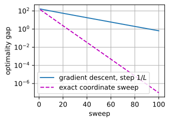
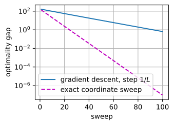
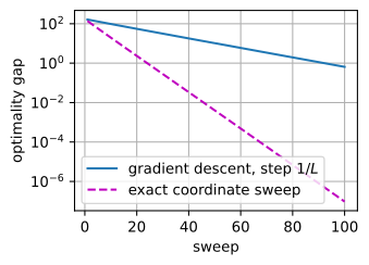
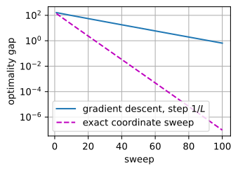
This coupled quadratic includes interactions between neighboring coordinates: changing one affects its neighbors. Even so, exact coordinate minimization uses the updated residual after each coordinate and converges faster per sweep here than the conservative global step \(1/L\). Different matrices can reverse that comparison; the point is the mechanism, not a universal ranking.
The same idea extends in two directions. Block coordinate descent updates a layer, feature group, or matrix block by solving a small subproblem, exploiting structure that scalar coordinates miss. For a composite objective \(f(\mathbf x)+\lambda\|\mathbf x\|_1\), the coordinate subproblem includes the nonsmooth term and its exact update is soft-thresholding, the proximal operator of Equation 26.3.14. This is why coordinate methods are natural for sparse regression and matrix factorization: each cheap local solve can create exact zeros, whereas an ordinary smooth gradient step cannot.
Coordinate descent is not the default for dense end-to-end neural training: accelerators are built for large matrix operations, not sequential scalar updates. It remains important for sparse linear models, embedding tables, alternating minimization, and inner problems where a block has a closed-form or very cheap solve.
26.3.5.6 Nonconvex Neural Networks
26.3.5.6.1 Structural Nonconvexity in Standard Parameterizations
The convexity calculus had one missing rule, composition with non-monotone nonlinear maps, and a neural network is built from repeated compositions. The loss surface of a deep network in its parameters is not convex, and a two-parameter “network” already shows why. Take \(f(a, b) = (ab - 1)^2\): a linear model with two stacked scalar weights and a squared loss. Its global minima form the hyperbola \(\{ab = 1\}\), a non-convex set. But our local-equals-global proposition proved the minimizer set of any convex function is convex; therefore \(f\) cannot be convex, and indeed the average of the minimizers \((1, 1)\) and \((-1, -1)\) is the origin, where \(f = 1\) sits strictly above the minimum \(0\). Standard neural networks have an analogous structural source of nonconvexity: permuting the hidden units of a layer (with their weights) leaves the computed function unchanged, so every minimum comes with combinatorially many symmetric copies scattered across parameter space. Generically the copies are distinct and averaging two of them raises the loss, exactly as the midpoint of \((1, 1)\) and \((-1, -1)\) did for \((ab - 1)^2\), and a minimizer set that contains distinct copies but not their averages cannot be convex. Standard multilayer parameterizations are therefore generally nonconvex.
26.3.5.6.2 A Formal Nonconvex Guarantee
Some linear-rate conclusions remain valid without convexity. The second half of the proof used only the inequality Equation 26.3.9, known as the Polyak–Łojasiewicz (PL) condition (after Polyak and Łojasiewicz, who introduced it independently in 1963 (Polyak 1963; Łojasiewicz 1963)):
\[ \begin{aligned} f \textrm{ is } L\textrm{-smooth} \;\;\textrm{and}\;\; \frac12\, \|\nabla f(\mathbf{x})\|^2 &\;\ge\; \mu \left( f(\mathbf{x}) - f^\star \right) \;\;\textrm{for all } \mathbf{x} \\ &\Longrightarrow \quad \textrm{GD converges linearly to } f^\star, \end{aligned} \]
with no convexity required (Karimi et al. 2016) (smoothness stays in the hypothesis; it is what powers the descent lemma half of the argument). PL says the gradient cannot be small unless the value is nearly optimal: stationary points must attain the global minimum value. Strong convexity implies PL (that was the first half of the proof), but the converse fails: PL functions can have multiple minima, plateaus of minimizers, and nonconvex curvature, as long as every stationary point is global. The standard example is \(f(x) = x^2 + 3\sin^2 x\), whose second derivative dips to \(-4\), so it is not convex, yet it satisfies PL globally. The cell verifies both claims on \([-5, 5]\) and then runs gradient descent, measuring the suboptimality gap \(f(x_k) - f^\star\) shrink by a near-constant factor per step, the signature of a linear rate.
f = lambda x: x**2 + 3 * np.sin(x)**2          # nonconvex; f* = 0 at x = 0
df = lambda x: 2 * x + 3 * np.sin(2 * x)
xs = np.linspace(-5, 5, 100001)
xs = xs[np.abs(xs) > 1e-3]                     # avoid 0/0 at the minimizer
print(f'PL constant on [-5, 5]: mu = {(0.5 * df(xs)**2 / f(xs)).min():.4f}')
print(f"min f'' = {(2 + 6 * np.cos(2 * xs)).min():.2f}  (f is not convex)")
x, gaps = 4.5, []
for _ in range(80):                            # gradient descent, eta = 1/16
    x -= df(x) / 16.0
    gaps.append(f(x))
ratios = np.array(gaps[1:]) / np.array(gaps[:-1])
print('successive gap ratios:', ratios[::16].round(4))
PL constant on [-5, 5]: mu = 0.1755
min f'' = -4.00 (f is not convex)
successive gap ratios: [0.6293 0.2907 0.25 0.25 0.25 ]The numerically measured PL constant on \([-5, 5]\) is \(\mu \approx 0.1755\): the function is non-convex (the minimum of \(f''\) is \(-4.00\)) yet PL. The window suffices for the global claim, because the ratio \(\tfrac12 f'(x)^2 / f(x)\) only grows outside it, tending to \(2\) as \(|x| \to \infty\); Exercise 7 completes the argument. Under gradient descent the successive gap ratios start at \(0.6293\) while the iterate crosses the slow middle stretch, then settle at exactly \(0.25\): a constant contraction, i.e. linear convergence, on a non-convex function. (The asymptotic \(0.25\) follows from the local quadratic approximation: near the minimum \(f\) looks like \(\tfrac12 f''(0) x^2\) with \(f''(0) = 8\), each step scales \(x\) by \(1 - 8/16 = \tfrac12\), and the gap is quadratic in \(x\).)
26.3.5.6.3 Model-Specific Analyses
For specified overparameterized models and initialization regimes, analyses can establish local PL-style inequalities near interpolation (Liu et al. 2022). Within the neighborhood where those assumptions remain valid, first-order methods may converge rapidly to a global training-loss minimum. This is not a generic property of neural networks and does not by itself imply a generalization guarantee.
26.3.5.6.4 Optimizer-Dependent Selection in Specific Models
Non-convexity has one more consequence the convex theory never had to face: the optimization procedure can determine which global minimum is reached. When many minimizers exist, gradient descent can select a systematic solution: it has an implicit bias. The simplest case is underdetermined least squares: started from \(\mathbf{w}_0 = \mathbf{0}\), every gradient \(X^\top(X\mathbf{w} - \mathbf{y})\) lies in the row space of \(X\), so the iterates never leave it, and the limit is the minimum-norm interpolant, the same solution the pseudoinverse computes (Section 24.3; Exercise 8 has you verify it, and Exercise 9 of Section 26.1 has you derive it). For logistic regression on separable data, gradient descent’s direction converges to the maximum-margin separator (Soudry et al. 2018), the SVM solution of Section 26.4. These examples show that an optimizer can select among multiple interpolating solutions. The selected solution can affect generalization, but the form of the implicit bias depends on the model, loss, initialization, and optimization dynamics.
Convex analysis applies directly to convex output-layer or auxiliary problems and supplies useful comparison results for nonconvex training. Outside its assumptions, however, its global guarantees do not transfer automatically; smoothness, PL conditions, and implicit-bias statements must be checked for the particular model and regime.
26.3.6 Summary
- A set is convex when every chord stays inside; half-spaces, norm balls, the simplex, and the PSD cone are the working catalog, and intersection preserves convexity (unions do not), which certifies the simplex, the PSD cone, and every polyhedral feasible set.
- A function is convex by any of three equivalent lenses: chord above graph, tangent below graph (the global under-estimator gradient methods exploit), or PSD Hessian. Strong convexity (\(\nabla^2 f \succeq \mu I\)) adds a curvature floor; subgradients extend the tangent lens to kinked losses like \(\ell_1\) and the hinge, with \(\partial |x|(0) = [-1, 1]\).
- Jensen’s inequality \(f(\mathbb{E}[X]) \le \mathbb{E}[f(X)]\) is the chord inequality lifted to expectations; its two-line proof is a supporting line plus linearity of expectation. It yields AM–GM, the ELBO gap, and \(D_{\mathrm{KL}} \ge 0\) with equality iff the distributions coincide, the cornerstone Section 28.1 builds on.
- For convex \(f\), every local minimum is global (and stationary \(\Rightarrow\) optimal); strict convexity gives uniqueness. Gradient descent’s local progress becomes a global rate: \(O(L\|\mathbf{x}_0 - \mathbf{x}^\star\|^2 / k)\) for smooth convex \(f\), and a linear rate \((1 - \mu/L)^k\) under strong convexity, both dimension-free.
- A short calculus (nonnegative sums, affine pre-composition, pointwise max, monotone composition) certifies hinge, \(\ell_1\), logistic, and softmax cross-entropy without touching a Hessian; log-sum-exp is convex because its Hessian is the softmax covariance, and its conjugate is negative entropy, the identity behind softmax-as-maximum-entropy and the variational duals of Chapter 28. Proximal operators generalize projections from sets to functions; soft-thresholding is the prox of \(\lambda|\cdot|\), and one prox per step (ISTA) optimizes kinked composite losses at gradient descent’s rate. Coordinate descent minimizes one coordinate or block at a time; on quadratics it is an exact one-dimensional solve, and with \(\ell_1\) regularization that solve becomes soft-thresholding.
- Deep networks are non-convex by construction (permutation symmetry makes the minimizer set non-convex), but the PL condition preserves linear convergence without convexity, and gradient descent’s implicit bias (min-norm, max-margin) decides which of the many minima you get.
26.3.7 Exercises
- Prove that every norm ball \(\{\mathbf{x} : \|\mathbf{x}\| \le r\}\) is convex directly from the triangle inequality, and exhibit two convex sets whose union is not convex. Then show the set of strictly positive definite matrices is convex, and explain why the PSD cone is its closure.
- Certify each of the following by naming the lens or calculus rule that does it in one line: (a) \(x \log x\) on \(x > 0\); (b) the hinge loss \(\sum_i \max(0, 1 - y_i\,\mathbf{w}^\top\mathbf{x}_i)\) in \(\mathbf{w}\);
- \(\|A\mathbf{x} - \mathbf{b}\|_1\); (d) the pointwise minimum of two convex functions: convex or not? Prove or give a counterexample.
- Compute the full subdifferential \(\partial f(x)\) of \(f(x) = |x|\) at every \(x \in \mathbb{R}\), and verify the optimality criterion \(0 \in \partial f(x^\star)\) picks out \(x^\star = 0\). Then show that for \(f(\mathbf{w}) = \tfrac12\|\mathbf{w} - \mathbf{z}\|^2 + \lambda\|\mathbf{w}\|_1\) the criterion yields the soft-thresholding solution \(w_i^\star = \mathrm{sign}(z_i) \max(|z_i| - \lambda, 0)\).
- Prove Jensen’s finite form \(f(\sum_i \theta_i \mathbf{x}_i) \le \sum_i \theta_i f(\mathbf{x}_i)\) by induction on the number of points, starting from the chord inequality. Use it (with \(-\log\)) to derive the full harmonic–geometric–arithmetic mean chain \(\textrm{HM} \le \textrm{GM} \le \textrm{AM}\) for positive numbers.
- A function is quasiconvex if all its sublevel sets are convex. Show every convex function is quasiconvex, and that \(x \mapsto \sqrt{|x|}\) is quasiconvex but not convex, so convex sublevel sets alone do not imply the chord inequality. Which step of the local-equals-global proof still works for quasiconvex functions, and which fails?
- In the \(O(1/k)\) proof, we observed that \(\|\mathbf{x}_t - \mathbf{x}^\star\|\) is nonincreasing. Verify this numerically for gradient descent on \(f(\mathbf{w}) = \tfrac12\|X\mathbf{w} - \mathbf{y}\|^2\) (reuse the data of the
#convexity-three-lensescell). The#convexity-rate-checkcell measured the value-gap contraction at \(\eta = 1/L\) and found exactly \((1 - \mu/L)^2\); predict what the contraction becomes at the more aggressive \(\eta = 2/(\mu + L)\) of Section 26.1, then verify by modifying the cell. - Show that the Polyak–Łojasiewicz condition Equation 26.3.9 implies every stationary point is a global minimizer, and that strong convexity implies PL (reproduce the proof). Then show PL does not imply convexity by verifying the PL inequality for \(f(x) = x^2 + 3\sin^2 x\) analytically on a neighborhood of \(0\), or numerically on \([-5, 5]\), as the
#convexity-pl-ratecell did. - Implicit bias, verified. Exercise 9 of Section 26.1 derives, on paper, that gradient descent on the underdetermined least-squares loss \(\tfrac12\|X\mathbf{w} - \mathbf{y}\|^2\) started at \(\mathbf{w}_0 = \mathbf{0}\) stays in the row space of \(X\) and converges to the minimum-\(\ell_2\)-norm interpolant \(X^+\mathbf{y}\). This exercise is the laboratory half: with a random \(4 \times 10\) system, (a) compare the GD limit against
np.linalg.pinv; (b) track the component of the iterates orthogonal to the row space and confirm it stays at exactly zero;- restart GD from a nonzero \(\mathbf{w}_0\) with a component off the row space. What changes in the limit, and why?
- Coordinate descent as Gauss–Seidel. Derive Equation 26.3.16, then show that one cyclic sweep is Gauss–Seidel applied to \(A\mathbf x=\mathbf b\). Modify the NumPy cell to use randomized coordinates, compare equal numbers of coordinate updates, and construct a matrix for which cyclic ordering is substantially worse.
26.3.8 Discussions
This section connects the preceding optimization analysis to the constrained problems that follow. Section 26.1 proved that smoothness alone gives stationarity; convexity upgrades those rates to global guarantees, and the PL condition showed how much of the upgrade survives without convexity. Section 26.4 draws on most of the above: convex feasible sets for projections, KKT sufficiency and Slater’s condition require convex objectives and constraints, the dual function’s concavity is the sup-of-affine rule, and its linear-constraint duals are convex conjugates. Beyond the chapter, Jensen’s inequality and the log-sum-exp/negative-entropy pair are the analytic engine of Section 28.1 and the variational bounds of Section 28.2, and the main book’s Section 9.1, Section 3.1, and Section 2.7 all stand on results proved here.