%matplotlib inline
from d2l import torch as d2l
import math
import torch
from torch import nn
from torch.nn import functional as F9.10 Batch Size
Batch size affects both gradient variance and hardware utilization. Section 9.3 showed that averaging \(b\) examples divides the variance by \(b\), while Section 9.4 showed that batching amortizes dispatch overhead until the device saturates. This leaves a quantitative question: when does increasing the batch cease to improve optimization? A larger batch costs proportionally more compute per step. If it removes noise the optimizer was actually fighting, the run takes proportionally fewer steps and total computation remains constant. Otherwise, it evaluates additional examples without reducing the number of steps. The transition depends on the optimization problem and changes during training.
This section makes the question quantitative. We define and measure the gradient-noise scale, the batch size at which the expected squared noise in a minibatch gradient equals the squared full-gradient norm; we run the defining experiment of large-batch training, steps to a fixed target loss as a function of batch size, on both of the chapter’s testbeds; we check the standard rules for moving the learning rate along with the batch and mark where they fail; and we look at how production language-model runs act on all of this by growing the batch during training. These experiments characterize the tradeoff between gradient variance and the number of examples processed.
%matplotlib inline
from d2l import jax as d2l
from flax import nnx
import jax
from jax import numpy as jnp
import math
import optax
9.10.1 The Gradient-Noise Scale
9.10.1.1 Signal versus Noise
Write \(\nabla f\) for the full-dataset gradient at the current parameters and \(\boldsymbol{\Sigma}\) for the covariance of a single example’s gradient, so that \(\operatorname{tr} \boldsymbol{\Sigma} = \mathbb{E}_i \|\nabla f_i - \nabla f\|^2\) is the total noise power carried by one example. A minibatch gradient \(\hat{\mathbf{g}}_b\) averaged over \(b\) examples drawn with replacement is unbiased, and its expected squared deviation from the truth is the \(1/b\) law we measured in Section 9.3: \(\mathbb{E}\|\hat{\mathbf{g}}_b - \nabla f\|^2 = \operatorname{tr} \boldsymbol{\Sigma} / b\). So every minibatch gradient is the sum of a signal of squared length \(\|\nabla f\|^2\), the same at every batch size, and a noise of squared length \(\operatorname{tr} \boldsymbol{\Sigma} / b\), which shrinks as the batch grows. The two parts change places at
\[b_{\textrm{noise}} = \frac{\operatorname{tr} \boldsymbol{\Sigma}}{\|\nabla f\|^2}, \tag{9.10.1}\]
the gradient-noise scale (McCandlish et al. 2018). Below \(b_{\textrm{noise}}\), the expected squared noise exceeds the squared signal, and doubling the batch halves that noise power. Above it, the signal dominates in this mean-square sense, so further averaging offers diminishing returns. The noise scale therefore predicts that increasing the batch up to roughly \(b_{\textrm{noise}}\) should reduce the number of steps without a large increase in total compute; beyond it, the compute cost should grow faster than the reduction in steps. The rest of this section tests that prediction.
9.10.1.2 A Two-Batch Estimator
Neither \(\operatorname{tr} \boldsymbol{\Sigma}\) nor \(\|\nabla f\|^2\) is observable from a single minibatch, but both fall out of a quantity that is: the squared norm of a minibatch gradient. Taking expectations of \(\|\hat{\mathbf{g}}_b\|^2 = \|\nabla f + (\hat{\mathbf{g}}_b - \nabla f)\|^2\) and using unbiasedness,
\[\mathbb{E}\big[\|\hat{\mathbf{g}}_b\|^2\big] = \|\nabla f\|^2 + \frac{\operatorname{tr} \boldsymbol{\Sigma}}{b}. \tag{9.10.2}\]
The expected squared norm of a minibatch gradient exceeds that of the true gradient by exactly the noise power. Measuring the mean squared norm at two batch sizes \(b_{\textrm{small}} < b_{\textrm{big}}\) gives two linear equations in the two unknowns, and solving them yields the estimator below. This is the measurement of Section 9.3 stripped of its crutch: there we needed the full-dataset gradient as ground truth; here two batch sizes suffice, which is what makes the noise scale cheap enough that large training runs log it continuously (in a data-parallel run, each worker’s local gradient supplies the small-batch norm for free).
We will measure both testbeds of this chapter: the Fashion-MNIST CNN of Section 9.6 and the TinyLM character-level transformer of Section 9.6.2, on its usual Time Machine data. The setup cell assembles the data as indexable tensors, so that a random index set gives a random minibatch. One caveat: minibatch indices are drawn independently from the empirical set, but adjacent Time Machine windows overlap by 63 of 64 characters. The estimator therefore treats highly redundant sequences as separate examples, so its numerical scale should be interpreted for this sampling scheme rather than as a count of independent pieces of text. For the language model one “example” is such a sequence, so its noise scale and batch sizes are denominated in sequences (tokens = sequences × 64).
device = d2l.try_gpu()
data = d2l.TimeMachine(batch_size=64, num_steps=64, tokenization='char',
                       num_train=100000)
X_lm = data.X[:data.num_train].to(device)
Y_lm = data.Y[:data.num_train].to(device)
fashion = d2l.FashionMNIST(batch_size=256)
X_f = (fashion.train.data.float() / 255).unsqueeze(1).to(device)
y_f = fashion.train.targets.to(device)

def make_cnn():
    return nn.Sequential(
        nn.LazyConv2d(32, kernel_size=3, padding=1), nn.ReLU(),
        nn.MaxPool2d(2),
        nn.LazyConv2d(64, kernel_size=3, padding=1), nn.ReLU(),
        nn.MaxPool2d(2),
        nn.Flatten(), nn.LazyLinear(128), nn.ReLU(), nn.LazyLinear(10))
data = d2l.TimeMachine(batch_size=64, num_steps=64, tokenization='char',
num_train=100000)
X_lm, Y_lm = data.X[:data.num_train], data.Y[:data.num_train]
fashion = d2l.FashionMNIST(batch_size=256)
X_f = jnp.asarray(fashion.train[0], jnp.float32)[..., None] / 255
y_f = jnp.asarray(fashion.train[1], jnp.int32)
class FashionCNN(nnx.Module):
def __init__(self, rngs=None):
rngs = nnx.Rngs(0) if rngs is None else rngs
self.conv1 = nnx.Conv(1, 32, kernel_size=(3, 3), rngs=rngs)
self.conv2 = nnx.Conv(32, 64, kernel_size=(3, 3), rngs=rngs)
self.fc1 = nnx.Linear(64 * 7 * 7, 128, rngs=rngs)
self.fc2 = nnx.Linear(128, 10, rngs=rngs)
def __call__(self, X):
X = nnx.max_pool(nnx.relu(self.conv1(X)), window_shape=(2, 2),
strides=(2, 2))
X = nnx.max_pool(nnx.relu(self.conv2(X)), window_shape=(2, 2),
strides=(2, 2))
X = X.reshape(X.shape[0], -1)
return self.fc2(nnx.relu(self.fc1(X)))The estimator follows Equation 9.10.2 line by line: average the squared gradient norm over many small minibatches and a few large ones, solve for the noise power and the signal power, return the ratio.
def grad_sq_norm(model, X, Y):
    logits = model(X)
    loss = F.cross_entropy(logits.reshape(-1, logits.shape[-1]),
                           Y.reshape(-1))
    grads = torch.autograd.grad(loss, list(model.parameters()))
    return sum((g ** 2).sum() for g in grads)

def noise_scale(model, X, Y, b_small=16, b_big=2048, m=400):
    def mean_sq_norm(b, m):
        idx = torch.randint(0, len(Y), (m, b), device=X.device)
        return torch.stack([grad_sq_norm(model, X[i], Y[i])
                            for i in idx]).mean()
    n_small, n_big = mean_sq_norm(b_small, m), mean_sq_norm(b_big, m // 8)
    tr_sigma = (n_small - n_big) / (1 / b_small - 1 / b_big)
    sq_norm = (b_big * n_big - b_small * n_small) / (b_big - b_small)
    return (tr_sigma / sq_norm).item()
def ce_loss(model, X, Y):
logits = model(X)
return optax.softmax_cross_entropy_with_integer_labels(
logits.reshape(-1, logits.shape[-1]), Y.reshape(-1)).mean()
@nnx.jit
def grad_sq_norm(model, X, Y):
grads = nnx.grad(ce_loss)(model, X, Y)
return sum((g ** 2).sum() for g in jax.tree.leaves(grads))
def noise_scale(model, X, Y, key, b_small=16, b_big=2048, m=400):
def mean_sq_norm(b, m, key):
idx = jax.random.randint(key, (m, b), 0, len(Y))
return jnp.stack([grad_sq_norm(model, X[i], Y[i])
for i in idx]).mean()
k1, k2 = jax.random.split(key)
n_small = mean_sq_norm(b_small, m, k1)
n_big = mean_sq_norm(b_big, m // 8, k2)
tr_sigma = (n_small - n_big) / (1 / b_small - 1 / b_big)
sq_norm = (b_big * n_big - b_small * n_small) / (b_big - b_small)
return float(tr_sigma / sq_norm)The noise scale depends on the current parameters, so when we measure matters. We measure twice: at initialization, and after 500 steps of Adam, using d2l.train_lm from Section 9.6 (which trains any model that maps inputs to logits, the CNN included). First the CNN:
torch.manual_seed(0)
cnn = make_cnn().to(device)
cnn(X_f[:2])  # Materialize the lazy layers
print(f'noise scale at initialization: {noise_scale(cnn, X_f, y_f):.0f}')
optimizer = torch.optim.Adam(cnn.parameters(), lr=0.004)
d2l.train_lm(cnn, fashion, optimizer, num_steps=500)
print(f'after 500 steps of Adam: {noise_scale(cnn, X_f, y_f):.0f}')
noise scale at initialization: 98
after 500 steps of Adam: 705cnn = FashionCNN(rngs=nnx.Rngs(0))
print(f'noise scale at initialization: '
f'{noise_scale(cnn, X_f, y_f, jax.random.PRNGKey(0)):.0f}')
optimizer = nnx.Optimizer(cnn, optax.adam(0.004), wrt=nnx.Param)
d2l.train_lm(cnn, fashion, optimizer, num_steps=500)
print(f'after 500 steps of Adam: '
f'{noise_scale(cnn, X_f, y_f, jax.random.PRNGKey(1)):.0f}')noise scale at initialization: 42
after 500 steps of Adam: 214Then the language model, with smaller probe batches because one example is already a 64-character sequence:
torch.manual_seed(0)
lm = d2l.TinyLM(len(data.vocab)).to(device)
print(f'noise scale at initialization: '
      f'{noise_scale(lm, X_lm, Y_lm, b_small=8, b_big=256):.1f}')
optimizer = torch.optim.Adam(lm.parameters(), lr=0.003)
d2l.train_lm(lm, data, optimizer, num_steps=500)
print(f'after 500 steps of Adam: '
      f'{noise_scale(lm, X_lm, Y_lm, b_small=8, b_big=256):.0f}')
noise scale at initialization: 2.5
after 500 steps of Adam: 113lm = d2l.TinyLM(len(data.vocab), rngs=nnx.Rngs(0))
ns_init = noise_scale(lm, X_lm, Y_lm, jax.random.PRNGKey(0),
b_small=8, b_big=256)
print(f'noise scale at initialization: {ns_init:.1f}')
optimizer = nnx.Optimizer(lm, optax.adam(0.002), wrt=nnx.Param)
d2l.train_lm(lm, data, optimizer, num_steps=500)
ns_500 = noise_scale(lm, X_lm, Y_lm, jax.random.PRNGKey(1),
b_small=8, b_big=256)
print(f'after 500 steps of Adam: {ns_500:.0f}')noise scale at initialization: 0.7
after 500 steps of Adam: 61Three readings, all of which we will use. First, the magnitudes: at these model and dataset sizes the noise scale is small — tens of examples for the CNN and single-digit sequence counts for the language model at initialization, rising to several hundred examples and on the order of a hundred sequences by step 500. The batch sizes used in the preceding experiments fall near or above these estimates, depending on the checkpoint. Second, the growth: within those 500 steps the CNN’s noise scale grows severalfold and the language model’s by one to two orders of magnitude, because the full-gradient norm is initially large relative to per-example disagreement and then decreases as the easiest improvements are exhausted. We return to this in the last part of the section, since it is the fact behind batch-size ramps. Third, the caveats: the estimate is itself noisy, increasingly so as \(\|\nabla f\|^2\) shrinks toward the noise floor of the estimator, and repeated runs scatter within a factor of about two, which is precise enough for choosing a batch size and not for much else. And the magnitude does not transfer across problems: the measurements of McCandlish et al. (2018) across workloads put the noise scale for large language models in the millions of tokens, against a few thousand characters here. What transfers is the concept and the growth during training, not the number.
9.10.2 Steps to a Target
The noise scale makes a falsifiable claim about training speed. To test it we use the standard experimental design of the large-batch literature (Shallue et al. 2019): fix a target loss, train at a range of batch sizes, and count the steps each needs to reach the target, along with the examples processed, which is steps times batch size. In the ideal noise-limited regime, doubling \(b\) should halve the step count and leave the example count unchanged; we call this perfect scaling. Once \(b\) passes the noise scale, further variance reduction does not materially reduce the step count. It approaches a floor \(S_{\min}\) set by the noiseless dynamics, so additional examples yield progressively smaller reductions in the step count. A simple model of a noisy quadratic (McCandlish et al. 2018) makes the whole trade-off a single hyperbola in the run-averaged noise scale:
\[ \frac{S(b)}{S_{\min}} = 1 + \frac{b_{\textrm{noise}}}{b}, \qquad \frac{E(b)}{E_{\min}} = 1 + \frac{b}{b_{\textrm{noise}}}, \tag{9.10.3}\]
with \(E(b) = b\, S(b)\) the examples consumed and \(E_{\min}\) the small-batch limit. Both formulas bend at the same place: at \(b = b_{\textrm{noise}}\), steps and examples each sit at twice their minimum. That elbow is the critical batch size, the largest batch that still converts additional computation into fewer sequential steps.
Our protocol, in full: the target is a fixed loss evaluated on a fixed subset of the training data every ten steps (evaluating on the noisy per-minibatch training loss would bias the small-batch runs, whose loss estimates fluctuate most). The optimizer is Adam. Its learning rate is tuned by a short grid at an anchor batch size \(b_0\) (64 sequences for the language model, 256 examples for the CNN) and moved across batch sizes by the square-root rule \(\eta(b) = \eta_0 \sqrt{b/b_0}\), a common heuristic for adaptive methods; the next part of this section states and verifies it. Each configuration uses one fixed seed, so the curves support qualitative comparisons rather than uncertainty estimates. The harness is train_lm from Section 9.6 with the stopping rule added:
def eval_loss(model, X, Y, chunk=4096):
    with torch.no_grad():
        losses = []
        for i in range(0, len(Y), chunk):
            logits = model(X[i:i + chunk])
            losses.append(F.cross_entropy(
                logits.reshape(-1, logits.shape[-1]),
                Y[i:i + chunk].reshape(-1)))
    return torch.stack(losses).mean().item()

def train_to_target(model, data, optimizer, X_eval, Y_eval, target,
                    max_steps, eval_every=10):
    model.to(device)
    step = 0
    while step < max_steps:
        for X, Y in data.train_dataloader():
            X, Y = X.to(device), Y.to(device)
            logits = model(X)
            loss = F.cross_entropy(logits.reshape(-1, logits.shape[-1]),
                                   Y.reshape(-1))
            optimizer.zero_grad()
            loss.backward()
            optimizer.step()
            step += 1
            if step % eval_every == 0 and \
               eval_loss(model, X_eval, Y_eval) <= target:
                return step
            if step >= max_steps:
                break
    return float('inf')
@nnx.jit
def eval_chunk(model, X, Y):
return ce_loss(model, X, Y)
def eval_loss(model, X, Y, chunk=4096):
return float(jnp.stack([eval_chunk(model, X[i:i + chunk],
Y[i:i + chunk])
for i in range(0, len(Y), chunk)]).mean())
def train_to_target(model, data, optimizer, X_eval, Y_eval, target,
max_steps, eval_every=10):
@nnx.jit
def step_fn(model, optimizer, X, Y):
loss, grads = nnx.value_and_grad(ce_loss)(model, X, Y)
optimizer.update(model, grads)
return loss
step = 0
while step < max_steps:
for X, Y in data.train_dataloader():
step_fn(model, optimizer, jnp.asarray(X), jnp.asarray(Y))
step += 1
if step % eval_every == 0 and \
eval_loss(model, X_eval, Y_eval) <= target:
return step
if step >= max_steps:
break
return float('inf')9.10.2.1 The Language Model
For TinyLM the target is a loss of 1.5 per character, a perplexity of about 4.5: well into learning, far from converged, and reachable at every batch size in this sweep within a minute. The batch sizes span two orders of magnitude in sequences.
lm_bs = [4, 16, 64, 256]
lm_steps = []
for b in lm_bs:
    torch.manual_seed(0)
    data_b = d2l.TimeMachine(batch_size=b, num_steps=64,
                             tokenization='char', num_train=100000)
    model = d2l.TinyLM(len(data_b.vocab))
    optimizer = torch.optim.Adam(model.parameters(),
                                 lr=0.003 * math.sqrt(b / 64))
    lm_steps.append(train_to_target(model, data_b, optimizer, X_lm[:2048],
                                    Y_lm[:2048], target=1.5,
                                    max_steps=8000))
    print(f'b={b:4d}  steps={lm_steps[-1]:6.0f}  '
          f'examples={b * lm_steps[-1]:8.0f}')
d2l.plot(lm_bs, [lm_steps, [lm_steps[0] * lm_bs[0] / b for b in lm_bs]],
         'batch size (sequences)', 'steps to loss 1.5', xscale='log',
         yscale='log', legend=['measured', 'perfect scaling'])
b= 4 steps= 4720 examples= 18880
b= 16 steps= 1180 examples= 18880
b= 64 steps= 390 examples= 24960
b= 256 steps= 190 examples= 48640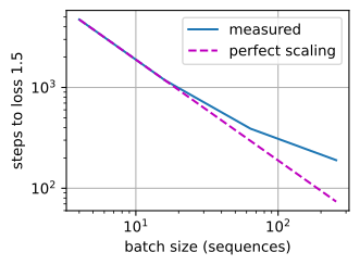
lm_bs = [4, 16, 64, 256]
lm_steps = []
for b in lm_bs:
    data_b = d2l.TimeMachine(batch_size=b, num_steps=64,
                             tokenization='char', num_train=100000)
    model = d2l.TinyLM(len(data_b.vocab), rngs=nnx.Rngs(0))
    optimizer = nnx.Optimizer(model,
                              optax.adam(0.002 * math.sqrt(b / 64)),
                              wrt=nnx.Param)
    lm_steps.append(train_to_target(model, data_b, optimizer, X_lm[:2048],
                                    Y_lm[:2048], target=1.5,
                                    max_steps=8000))
    print(f'b={b:4d}  steps={lm_steps[-1]:6.0f}  '
          f'examples={b * lm_steps[-1]:8.0f}')
d2l.plot(lm_bs, [lm_steps, [lm_steps[0] * lm_bs[0] / b for b in lm_bs]],
         'batch size (sequences)', 'steps to loss 1.5', xscale='log',
         yscale='log', legend=['measured', 'perfect scaling'])
b= 4 steps= 4680 examples= 18720
b= 16 steps= 1540 examples= 24640
b= 64 steps= 640 examples= 40960
b= 256 steps= 440 examples= 112640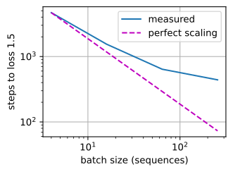
From \(b=4\) to \(b=16\), the measured curve remains close to the perfect-scaling reference and the example count changes little. By \(b=256\), the measured curve is above the reference — steps still fall, but each quadrupling of the batch now reduces the step count by half or less, not the fourfold cut of perfect scaling, and the examples consumed have more than doubled and are climbing. The elbow sits between a few tens and a couple of hundred sequences, within a small factor of the noise scale we measured mid-training, which is all Equation 9.10.3 promises for so coarse an estimate.
9.10.2.2 The CNN
The identical experiment on the CNN, with a target loss of 0.35 and batch sizes from 8 to 2048:
cnn_bs = [8, 32, 128, 512, 2048]
cnn_steps = []
for b in cnn_bs:
    torch.manual_seed(0)
    fashion_b = d2l.FashionMNIST(batch_size=b)
    model = make_cnn()
    optimizer = torch.optim.Adam(model.parameters(),
                                 lr=0.004 * math.sqrt(b / 256))
    cnn_steps.append(train_to_target(model, fashion_b, optimizer,
                                     X_f[:8192], y_f[:8192], target=0.35,
                                     max_steps=8000))
    print(f'b={b:4d}  steps={cnn_steps[-1]:6.0f}  '
          f'examples={b * cnn_steps[-1]:8.0f}')
d2l.plot(cnn_bs, [cnn_steps,
                  [cnn_steps[0] * cnn_bs[0] / b for b in cnn_bs]],
         'batch size', 'steps to loss 0.35', xscale='log', yscale='log',
         legend=['measured', 'perfect scaling'])
b= 8 steps= 2510 examples= 20080
b= 32 steps= 640 examples= 20480
b= 128 steps= 220 examples= 28160
b= 512 steps= 110 examples= 56320
b=2048 steps= 120 examples= 245760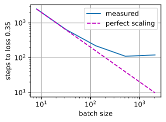
cnn_bs = [8, 32, 128, 512, 2048]
cnn_steps = []
for b in cnn_bs:
    fashion_b = d2l.FashionMNIST(batch_size=b)
    model = FashionCNN(rngs=nnx.Rngs(0))
    optimizer = nnx.Optimizer(model,
                              optax.adam(0.004 * math.sqrt(b / 256)),
                              wrt=nnx.Param)
    cnn_steps.append(train_to_target(model, fashion_b, optimizer,
                                     X_f[:8192], y_f[:8192], target=0.35,
                                     max_steps=8000))
    print(f'b={b:4d}  steps={cnn_steps[-1]:6.0f}  '
          f'examples={b * cnn_steps[-1]:8.0f}')
d2l.plot(cnn_bs, [cnn_steps,
                  [cnn_steps[0] * cnn_bs[0] / b for b in cnn_bs]],
         'batch size', 'steps to loss 0.35', xscale='log', yscale='log',
         legend=['measured', 'perfect scaling'])
b= 8 steps= 1990 examples= 15920
b= 32 steps= 490 examples= 15680
b= 128 steps= 170 examples= 21760
b= 512 steps= 70 examples= 35840
b=2048 steps= 60 examples= 122880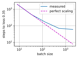
The CNN shows a similar pattern: the first quadrupling remains near the reference line, after which the gap widens. At the top of the range a further quadrupling of the batch (a quadrupling of the compute per step) cuts the step count by at most a third, and in some runs the count rises instead, a sign we will explain in the next part. By then the example count is several times its small-batch minimum: additional compute still reduces sequential steps, but with substantially lower data efficiency.
9.10.2.3 Examples Required to Reach the Target
Replotting both sweeps as examples-to-target puts the two testbeds on one axis and states the cost of parallelism directly:
d2l.plot([lm_bs, cnn_bs],
         [[b * s for b, s in zip(lm_bs, lm_steps)],
          [b * s for b, s in zip(cnn_bs, cnn_steps)]],
         'batch size', 'examples to target', xscale='log', yscale='log',
         legend=['TinyLM', 'Fashion-MNIST CNN'])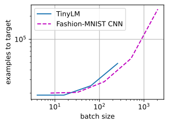
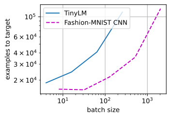
Each curve is approximately flat in the efficient small-batch regime and bends upward near its critical batch size, as Equation 9.10.3 predicts. Each point represents a different tradeoff: more total compute can buy fewer sequential steps and, with sufficient hardware, less wall-clock time. Below the elbow, that tradeoff is favorable; above it, progressively more compute is required for each further reduction in steps. Where a given team should sit depends on what is scarce, accelerators or days, which is why frontier runs crowd as close to their critical batch size as their clusters allow and why the exercises ask you to trace this Pareto frontier explicitly.
9.10.3 Learning-Rate Rules
Changing the batch size changes the optimization problem the learning rate was tuned for, so \(\eta\) has to move with \(b\); running the sweep above at a fixed \(\eta\) would have confounded batch statistics with step-size mistuning. Two rules cover practice:
\[ \eta(b) = \frac{b}{b_0}\, \eta_0 \;\; \textrm{(SGD)}, \qquad \eta(b) = \sqrt{\frac{b}{b_0}}\, \eta_0 \;\; \textrm{(adaptive methods)}. \tag{9.10.4}\]
The linear rule for SGD (Goyal et al. 2017) follows from the noise-floor picture of Section 9.3: there we saw SGD stall in a noise ball whose squared radius is proportional to \(\eta\) times the gradient variance. A batch of \(b\) divides the variance by \(b\), so holding \(\eta / b\) fixed holds the noise ball fixed, and with it the whole stochastic character of the trajectory. It is also the small-batch limit of the optimal step size in the noisy-quadratic model, \(\eta_{\textrm{opt}}(b) = \eta_{\max} / (1 + b_{\textrm{noise}}/b)\): linear in \(b\) while \(b \ll b_{\textrm{noise}}\), saturating at \(\eta_{\max}\) beyond it — the rule announces its own expiry at the noise scale. For Adam and its relatives the scaling is weaker. The preconditioner already divides each coordinate by its root-mean-square gradient, which itself shrinks as the batch quiets the noise. The stochastic-differential-equation analysis of Malladi et al. (2022) makes the scaling precise: growing the batch by a factor \(k\) preserves Adam’s dynamics if every time constant moves together — \(\eta' = \sqrt{k}\,\eta\), \(\beta_i' = 1 - k(1 - \beta_i)\), \(\epsilon' = \epsilon / \sqrt{k}\) — which is possible only while \(k(1 - \beta_i) < 1\), i.e. \(k < 10\) at \(\beta_1 = 0.9\). Common practice, and the sweeps above, move \(\eta\) alone; changing only \(\eta\) gives the commonly used square-root heuristic rather than exact preservation of the full dynamics, and Equation 9.10.4 states it in that everyday form.
We verify both rules on the CNN with the chapter’s usual instrument, a learning-rate grid, trained at \(b=8\) and \(b=64\) on a fixed budget of 12,800 examples so that both batch sizes see the same data. If a rule holds, the whole loss-versus-\(\eta\) curve should shift right by the predicted factor — \(8\times\) for SGD, \(\sqrt{8} \approx 2.8\times\) for Adam — when the batch grows \(8\times\). Since d2l.train_lm is already a fixed-step trainer, the sweep is a few lines:
def final_loss_at(make_optimizer, lrs, b, num_examples=12800):
    data_b = d2l.FashionMNIST(batch_size=b)
    final = []
    for lr in lrs:
        torch.manual_seed(0)
        model = make_cnn().to(device)
        model(X_f[:2])  # Materialize the lazy layers
        d2l.train_lm(model, data_b, make_optimizer(model, lr),
                     num_steps=num_examples // b)
        loss = eval_loss(model, X_f[:8192], y_f[:8192])
        final.append(loss if math.isfinite(loss) else float('nan'))
        print(f'b={b:3d}  lr={lr:g}  loss={final[-1]:.3f}')
    return final
def final_loss_at(make_tx, lrs, b, num_examples=12800):
data_b = d2l.FashionMNIST(batch_size=b)
final = []
for lr in lrs:
model = FashionCNN(rngs=nnx.Rngs(0))
optimizer = nnx.Optimizer(model, make_tx(lr), wrt=nnx.Param)
d2l.train_lm(model, data_b, optimizer,
num_steps=num_examples // b)
loss = eval_loss(model, X_f[:8192], y_f[:8192])
final.append(loss if math.isfinite(loss) else float('nan'))
print(f'b={b:3d} lr={lr:g} loss={final[-1]:.3f}')
return finalsgd_lrs = [0.003125, 0.00625, 0.0125, 0.025, 0.05, 0.1, 0.2]
make_sgd = lambda model, lr: torch.optim.SGD(model.parameters(), lr,
momentum=0.9)
sgd_small = final_loss_at(make_sgd, sgd_lrs, b=8)
sgd_big = final_loss_at(make_sgd, sgd_lrs, b=64)
d2l.plot(sgd_lrs, [sgd_small, sgd_big], 'learning rate', 'final loss',
xscale='log', legend=['b=8', 'b=64'])b= 8 lr=0.003125 loss=0.594
b= 8 lr=0.00625 loss=0.518
b= 8 lr=0.0125 loss=0.515
b= 8 lr=0.025 loss=0.554
b= 8 lr=0.05 loss=1.554
b= 8 lr=0.1 loss=2.321
b= 8 lr=0.2 loss=2.347
b= 64 lr=0.003125 loss=0.787
b= 64 lr=0.00625 loss=0.687
b= 64 lr=0.0125 loss=0.614
b= 64 lr=0.025 loss=0.563
b= 64 lr=0.05 loss=0.451
b= 64 lr=0.1 loss=0.465
b= 64 lr=0.2 loss=0.693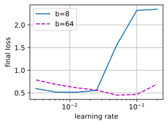
sgd_lrs = [0.003125, 0.00625, 0.0125, 0.025, 0.05, 0.1, 0.2]
sgd_small = final_loss_at(lambda lr: optax.sgd(lr, momentum=0.9),
                          sgd_lrs, b=8)
sgd_big = final_loss_at(lambda lr: optax.sgd(lr, momentum=0.9),
                        sgd_lrs, b=64)
d2l.plot(sgd_lrs, [sgd_small, sgd_big], 'learning rate', 'final loss',
         xscale='log', legend=['b=8', 'b=64'])
b= 8 lr=0.003125 loss=0.435
b= 8 lr=0.00625 loss=0.452
b= 8 lr=0.0125 loss=0.398
b= 8 lr=0.025 loss=0.413
b= 8 lr=0.05 loss=1.416
b= 8 lr=0.1 loss=2.325
b= 8 lr=0.2 loss=2.382
b= 64 lr=0.003125 loss=0.674
b= 64 lr=0.00625 loss=0.548
b= 64 lr=0.0125 loss=0.484
b= 64 lr=0.025 loss=0.422
b= 64 lr=0.05 loss=0.428
b= 64 lr=0.1 loss=0.412
b= 64 lr=0.2 loss=0.629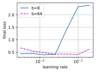
adam_lrs = [0.0002, 0.0004, 0.0008, 0.0016, 0.0032, 0.0064, 0.0128,
            0.0256]
make_adam = lambda model, lr: torch.optim.Adam(model.parameters(), lr)
adam_small = final_loss_at(make_adam, adam_lrs, b=8)
adam_big = final_loss_at(make_adam, adam_lrs, b=64)
d2l.plot(adam_lrs, [adam_small, adam_big], 'learning rate', 'final loss',
         xscale='log', legend=['b=8', 'b=64'])
b= 8 lr=0.0002 loss=0.519
b= 8 lr=0.0004 loss=0.476
b= 8 lr=0.0008 loss=0.450
b= 8 lr=0.0016 loss=0.426
b= 8 lr=0.0032 loss=0.429
b= 8 lr=0.0064 loss=0.455
b= 8 lr=0.0128 loss=0.558
b= 8 lr=0.0256 loss=0.599
b= 64 lr=0.0002 loss=0.630
b= 64 lr=0.0004 loss=0.563
b= 64 lr=0.0008 loss=0.501
b= 64 lr=0.0016 loss=0.439
b= 64 lr=0.0032 loss=0.408
b= 64 lr=0.0064 loss=0.395
b= 64 lr=0.0128 loss=0.452
b= 64 lr=0.0256 loss=0.508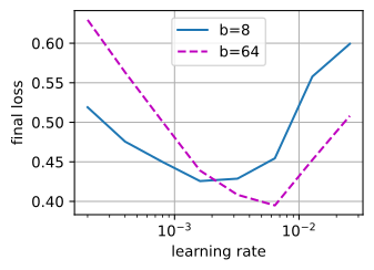
adam_lrs = [0.0002, 0.0004, 0.0008, 0.0016, 0.0032, 0.0064, 0.0128,
            0.0256]
adam_small = final_loss_at(optax.adam, adam_lrs, b=8)
adam_big = final_loss_at(optax.adam, adam_lrs, b=64)
d2l.plot(adam_lrs, [adam_small, adam_big], 'learning rate', 'final loss',
         xscale='log', legend=['b=8', 'b=64'])
b= 8 lr=0.0002 loss=0.436
b= 8 lr=0.0004 loss=0.449
b= 8 lr=0.0008 loss=0.398
b= 8 lr=0.0016 loss=0.370
b= 8 lr=0.0032 loss=0.395
b= 8 lr=0.0064 loss=0.512
b= 8 lr=0.0128 loss=0.490
b= 8 lr=0.0256 loss=0.744
b= 64 lr=0.0002 loss=0.515
b= 64 lr=0.0004 loss=0.472
b= 64 lr=0.0008 loss=0.441
b= 64 lr=0.0016 loss=0.418
b= 64 lr=0.0032 loss=0.413
b= 64 lr=0.0064 loss=0.422
b= 64 lr=0.0128 loss=0.393
b= 64 lr=0.0256 loss=0.534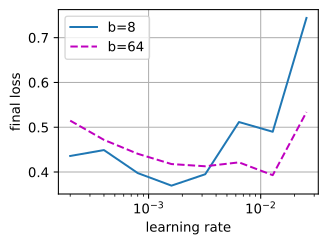
Both plots have a broad minimum and a sharp increase on the right, and growing the batch slides the basin rightward. For SGD the best region moves by roughly the batch ratio, a factor of four to eight in our runs — retuning from scratch at \(b=64\) finds nothing better than what the linear rule predicts from \(b=8\). For Adam the basin moves by only a factor of about two to four; applying the linear rule to Adam (\(8\times\), the rightmost points of the upper curve) lands measurably past the optimum. The basins are broad, which is itself worth remembering: near the optimum, being wrong by a factor of two costs little, and the rules are aids for crossing large batch-size ratios, not precision instruments.
9.10.3.1 Where the Rules Break
The rules fail in three characteristic places, and each failure is visible somewhere in this section’s data. Past the noise scale: both rules assume the run is noise-limited; once \(b\) approaches \(b_{\textrm{noise}}\) the optimal step stops growing, and continuing to scale \(\eta\) can overshoot. The upturn at the top of the steps-to-target sweeps is consistent with this mechanism, and the exercises reproduce it in isolation. Against the stability ceiling: the largest usable \(\eta\) is capped by curvature, as we saw for gradient descent in Section 9.2, and the cap does not move with the batch. When we first ran the SGD sweep at batch sizes of a few hundred, both basins pinned against the same stability limit, and the optimum stopped moving; scaling rules only operate in the room below the ceiling. Early in training: at initialization the noise scale is at its smallest and curvature effects at their worst, so a large batch with a linearly scaled \(\eta\) can diverge in the first steps. The practical fix is learning-rate warmup, which Goyal et al. (2017) introduced for exactly this reason; Section 9.8 covers it. Finally, none of this is a universal law: measured across many workloads, the curves of Equation 9.10.3 hold their shape but their elbows range over orders of magnitude with architecture, dataset, and optimizer (Shallue et al. 2019). Large batches were once also blamed for a generalization gap — converging to sharp minima that test poorly (Keskar et al. 2017) — but much of that gap closes under full retuning of \(\eta\) and training length; the durable cost of a large batch is data efficiency, which is what this section measured.
9.10.4 Growing the Batch
The noise scale is not a constant of the problem. We measured it growing within the first 500 steps (severalfold for the CNN, one to two orders of magnitude for the language model), and the mechanism operates at every scale: \(\|\nabla f\|\) decreases as the easiest progress is made, while per-example disagreement persists. A fixed batch therefore cannot remain equally compute-efficient throughout training: a batch chosen for the end may exceed the smaller critical batch size near the beginning. Several large language-model runs address this with a batch-size ramp. GPT-3 grew its batch from 32 thousand to 3.2 million tokens over the first billions of tokens of training (Brown et al. 2020). Llama 3 doubled its batch twice on a fixed schedule, from 4 million to 16 million tokens, as training progressed (Grattafiori et al. 2024). DeepSeek-V3 ramped from about 3 thousand to 15 thousand sequences across the first half-trillion tokens (DeepSeek-AI et al. 2024). What these schedules set by hand, measurement can set directly: researchers at Ai2 measured the critical batch size as training proceeded and doubled the batch each time the measurement overtook it, finding that the critical batch size tracks the loss reached — the data scale — far more than the model size (Merrill et al. 2025), in line with other measurements of how the elbow moves during pretraining (Zhang et al. 2024).
Two interactions are worth carrying forward. First, with the schedule: in the simple SGD noise-floor model, raising \(b\) at fixed \(\eta\) reduces the stochastic contribution through the same ratio \(\eta/b\) as lowering \(\eta\) at fixed \(b\). A batch ramp can therefore provide some of the noise-reduction effect of learning-rate decay (Smith et al. 2018), and the ramp and the schedule of Section 9.8 must be designed together, not tuned as independent knobs. Second, with the optimizer: the descent-direction decision feeds back into the noise-management one. Measurements on the studied pretraining workloads find that Muon sustains data efficiency to larger batch sizes than AdamW (Shah et al. 2025), effectively moving the elbow of Equation 9.10.3 to the right; Section 9.9 takes up why. One boundary remains. This section measures a large batch in examples; turning the fewer, larger steps into less wall-clock time requires splitting each batch across many devices, and that is data parallelism, the subject of Chapter 13.
9.10.5 Summary
A minibatch gradient is signal plus noise, and the two trade places at the gradient-noise scale \(b_{\textrm{noise}} = \operatorname{tr} \boldsymbol{\Sigma} / \|\nabla f\|^2\), measurable with nothing more than gradient norms at two batch sizes. Below it, doubling the batch halves the steps to a target at constant total compute; above it, steps flatten at a floor and examples are wasted — both testbeds showed the predicted hyperbola, with the elbow within a small factor of the measured noise scale. Moving between batch sizes requires moving the learning rate: with the batch ratio for SGD, with its square root for adaptive methods, valid below the noise scale and under the stability ceiling, with warmup protecting the early steps. The noise scale grows as the loss falls, which is why serious runs grow their batch during training rather than fixing it.
9.10.6 Exercises
- [code] The noise scale over training.
noise_scaleof Section 9.10.1.2 measuredTinyLMat initialization and after 500 steps of Adam. Repeat that run for 3,000 steps and measure the noise scale at steps 0, 25, 50, 100, 200, 500, 1,000, 2,000, and 3,000. At each checkpoint also record the loss thateval_lossreports onX_lm[:2048]andY_lm[:2048].- Plot the noise scale against this loss. Does the growth continue, slow down, or reverse?
- Under the rule of Section 9.10.4, doubling \(b\) whenever \(b_{\textrm{noise}}\) overtakes it, and starting from \(b = 4\), at which losses would the doublings land? Interpolate \(\log b_{\textrm{noise}}\) linearly in the loss between checkpoints. Explain why the step counts of this run at \(b = 64\) would not tell a ramped run when to double.
- [code] Past the elbow. Extend the
TinyLMsweep of Section 9.10.2 to \(b = 1024\) under the square-root rule of Equation 9.10.4, then rerun \(b = 1024\) with \(\eta\) held at its \(b = 256\) value.- How do the step counts of the two \(b = 1024\) runs compare with each other and with the \(b = 256\) run?
- Explain both observations with Equation 9.10.3 and the saturating optimal step size \(\eta_{\textrm{opt}}(b) = \eta_{\max} / (1 + b_{\textrm{noise}}/b)\).
- [code] The factor-of-two check. ● Equation Equation 9.10.3 predicts that examples-to-target reach twice their minimum at \(b = b_{\textrm{noise}}\), where \(b_{\textrm{noise}}\) is averaged over the run.
- From the checkpoints of the first problem, average \(b_{\textrm{noise}}\) over the training steps before the loss first falls to \(1.5\), interpolating linearly between checkpoints.
- Interpolate \(\log (b\, S(b))\) linearly in \(\log b\) from
lm_bsandlm_steps, and find the batch size at which \(b\, S(b)\) reaches twice its smallest measured value. By what factor does this elbow differ from the average of the first sub-item? - Repeat the sweep and the checkpoint measurements with a second seed. Is the gap between the two estimates larger than the seed-to-seed scatter of each?
- [code] Retuning instead of scaling. The CNN sweep recorded in
cnn_bsandcnn_stepsmoved \(\eta\) by the square-root rule rather than retuning. For each batch size, run a three-point learning-rate grid spaced by factors of two around the rule’s value and keep the best steps-to-target. Which points of the curve move, and does the elbow? - Time-optimal and compute-optimal batch size. Suppose one optimizer step at batch size \(b\) takes \(t(b) = t_0 (1 + b / b_{\textrm{sat}})\) seconds, where \(b_{\textrm{sat}}\) is the batch size that saturates the device. Time-to-target is then \(T(b) = t(b)\, S(b)\), and compute-to-target is the example count \(E(b) = b\, S(b)\), which by Equation 9.10.3 is smallest at the smallest batch. Using Equation 9.10.3, find the batch size that minimizes \(T(b)\), and express its \(E(b)\) as a multiple of \(E_{\min}\).
- [extended] Measured time-compute tradeoff. ● The step-time model \(t(b)\) of the previous problem has two constants, \(t_0\) and \(b_{\textrm{sat}}\), that depend on the hardware.
- Measure \(t_0\) and \(b_{\textrm{sat}}\) for
TinyLMon your hardware withd2l.Timerby timing steps at several batch sizes. - Combine \(t(b)\) with
lm_bsandlm_stepsand plot \(T(b)\) against \(E(b)\). Compare the time-optimal batch size on this curve with the prediction of the previous problem, evaluated at the run-averaged \(b_{\textrm{noise}}\) of the third problem. By what factor does the time-optimal batch cut \(T(b)\) relative to \(b = 4\), and by what factor does it raise \(E(b)\)?
- Measure \(t_0\) and \(b_{\textrm{sat}}\) for
- [code] Noise scale per population. ● The census of Section 9.6.2 splits
TinyLM’s parameters into embeddings, matrices, and vectors. Restrictgrad_sq_normto one population at a time and measure its noise scale withnoise_scale, at initialization and after 500 steps of Adam.- Which population has the largest noise scale, and does the ranking change during training?
- The census describes embedding rows as receiving gradients only when their token occurs. Count the rows of
token_emband ofpos_embthat receive no gradient in a probe minibatch of 8 sequences, and state whether this sparsity can account for the embeddings’ noise scale. - What does the ranking imply for one global batch size serving all three populations?