import numpy as np
import torch24.2 Eigendecompositions
In Section 24.1, a matrix was interpreted as a linear transformation that rotates, skews, and rescales space. Eigenvalues identify directions, called eigenvectors, along which this transformation is pure scaling. When the eigenvectors form a basis, the transformation separates into independent one-dimensional scalings. This representation is useful for stability analysis, PCA, and loss curvature. We develop it through geometric examples and algebraic results, using iterated linear maps to show how repeated matrix application depends on the spectrum.
The numerical checks in this section use small dense matrices.
import numpy as np
import tensorflow as tf
import numpy as np
import jax
jax.config.update("jax_enable_x64", True) # honor explicit float64 (else JAX
# silently truncates to float32 and the eigvals/power-iteration check disagrees)
from jax import numpy as jnpimport numpy as np24.2.1 Eigenvalues and Eigenvectors
24.2.1.1 Definition and Geometry
Suppose that we have a matrix \(\mathbf{A}\) with the following entries:
\[ \mathbf{A} = \begin{bmatrix} 2 & 0 \\ 0 & -1 \end{bmatrix}. \]
If we apply \(\mathbf{A}\) to any vector \(\mathbf{v} = [x, y]^\top\), we obtain a vector \(\mathbf{A}\mathbf{v} = [2x, -y]^\top\). This has an intuitive interpretation: stretch the vector to be twice as wide in the \(x\)-direction, and then flip it in the \(y\)-direction.
However, there are some vectors for which the direction remains unchanged. Namely \([1, 0]^\top\) gets sent to \([2, 0]^\top\) and \([0, 1]^\top\) gets sent to \([0, -1]^\top\). These vectors are still on the same line through the origin; the only modification is that \(\mathbf{A}\) scales \([1,0]^\top\) by \(2\) and \([0,1]^\top\) by \(-1\). We call such vectors eigenvectors and the factor they are stretched by their eigenvalues.
In general, if we can find a number \(\lambda\) and a nonzero vector \(\mathbf{v}\) such that
\[ \mathbf{A}\mathbf{v} = \lambda \mathbf{v}, \tag{24.2.1}\]
we say that \(\mathbf{v}\) is an eigenvector of \(\mathbf{A}\) and \(\lambda\) its eigenvalue. (We insist \(\mathbf{v}\neq\mathbf 0\): the zero vector trivially satisfies Equation 24.2.1 for every \(\lambda\) and carries no information. The scalar \(\lambda\) is allowed to be zero, and we will see that \(\lambda=0\) signals a non-invertible matrix.) For a fixed eigenvalue \(\lambda\), the set of all vectors satisfying \(\mathbf{A}\mathbf{v}=\lambda\mathbf{v}\), together with \(\mathbf 0\), forms a subspace, the eigenspace of \(\lambda\).
The image of the unit circle is an ellipse, or a lower-dimensional segment or point when the matrix is singular. For a general matrix, however, the input directions and output axes of this ellipse are its right and left singular vectors, not necessarily its eigenvectors. The two coincide for the symmetric examples below: their ellipse axes lie along orthonormal eigenvectors, with half-lengths \(|\lambda_i|\) and an orientation reversal when \(\lambda_i<0\). Figure 24.2.1 draws \(\operatorname{diag}(2,-1)\) and \([[2,1],[1,2]]\). The SVD in Section 24.3 retains this picture for every matrix by allowing distinct orthonormal bases for the input and output spaces.
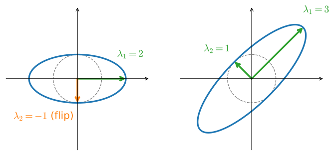
The green arrows are the unit eigenvectors; the red arrows are their images \(\mathbf{A}\mathbf{v}_i=\lambda_i\mathbf{v}_i\), which fall exactly on the ellipse’s axes. For \(\operatorname{diag}(2,-1)\) the axes are the coordinate directions; for the symmetric \([[2,1],[1,2]]\) they are the diagonal directions \([1,1]^\top/\sqrt2\) (scaled by \(3\)) and \([1,-1]^\top/\sqrt2\) (scaled by \(1\)).
24.2.1.2 Finding Eigenvalues
To find the eigenvalues, subtract \(\lambda\mathbf v\) from both sides of Equation 24.2.1 and factor out the vector. This gives
\[(\mathbf{A} - \lambda \mathbf{I})\mathbf{v} = 0. \tag{24.2.2}\]
Because \(\mathbf v\) must be nonzero, this equation has a solution precisely when \(\mathbf{A}-\lambda\mathbf I\) has a nontrivial null space. Equivalently, the matrix is singular and \(\det(\mathbf{A}-\lambda\mathbf I)=0\). The eigenvalues are the roots of this equation. For each root, solving \(\mathbf{A}\mathbf{v} = \lambda \mathbf{v}\) gives the corresponding eigenspace.
Consider the matrix
\[ \mathbf{A} = \begin{bmatrix} 2 & 1\\ 2 & 3 \end{bmatrix}. \]
The equation \(\det(\mathbf{A}-\lambda \mathbf{I}) = 0\) is a polynomial equation in \(\lambda\): the characteristic polynomial \(p(\lambda) = \det(\mathbf{A}-\lambda\mathbf{I})\), here \((2-\lambda)(3-\lambda)-2 = (4-\lambda)(1-\lambda)\). Thus the two eigenvalues are \(\lambda = 1\) and \(\lambda = 4\). To find the associated eigenvectors, we solve \((\mathbf{A}-\mathbf{I})\mathbf{v}=\mathbf 0\) for \(\lambda = 1\) and \((\mathbf{A}-4\mathbf{I})\mathbf{v}=\mathbf 0\) for \(\lambda = 4\), i.e.
\[ \begin{bmatrix} 2 & 1\\ 2 & 3 \end{bmatrix}\begin{bmatrix}x \\ y\end{bmatrix} = \begin{bmatrix}x \\ y\end{bmatrix} \; \textrm{and} \; \begin{bmatrix} 2 & 1\\ 2 & 3 \end{bmatrix}\begin{bmatrix}x \\ y\end{bmatrix} = \begin{bmatrix}4x \\ 4y\end{bmatrix} . \]
These are solved (up to scale) by \([1, -1]^\top\) for \(\lambda = 1\) and \([1, 2]^\top\) for \(\lambda = 4\), respectively. (Each eigenvector is determined only up to a nonzero scalar multiple: if \(\mathbf v\) is an eigenvector, so is \(c\mathbf v\) for any \(c\neq0\), since both sides of Equation 24.2.1 scale by \(c\).)
We can check this in code using the built-in eig routine.
import numpy as onp
onp.linalg.eig(onp.array([[2, 1], [2, 3]]))
EigResult(eigenvalues=array([1., 4.]), eigenvectors=array([[-0.70710678, -0.4472136 ],
[ 0.70710678, -0.89442719]]))MXNet arrays have no complex dtype, so mxnet.np.linalg.eig fails whenever the spectrum is complex, as it is for some matrices later in this section; we therefore use plain NumPy for eigenvalue computations here.
The library normalizes the eigenvectors to have length one, whereas we took ours to be of arbitrary length. Additionally, the choice of sign is arbitrary. However, the vectors computed are parallel to the ones we found by hand with the same eigenvalues.
What does eig compute? For \(n\ge5\) there is no formula in radicals for the roots of the characteristic polynomial, and practical libraries never form that polynomial anyway. They instead reduce \(\mathbf{A}\) to a nearly-triangular Hessenberg form and run the shifted QR algorithm, an iteration that drives the matrix toward triangular form while preserving its eigenvalues (Golub and Van Loan 1996). The iteration targets triangular form because a triangular matrix displays its eigenvalues on its diagonal: \(\mathbf{T}-\lambda\mathbf{I}\) is again triangular, so by the triangular determinant rule of Section 24.1.4.4.1, \(\det(\mathbf{T}-\lambda\mathbf{I})=\prod_i(t_{ii}-\lambda)\), which vanishes exactly at the diagonal values. The power iteration we develop later in this section matters in the complementary regime, when \(\mathbf{A}\) is too large to factor and only matrix–vector products are affordable.
24.2.1.3 Eigendecomposition and What It Computes
Continue the preceding example. Let
\[ \mathbf{W} = \begin{bmatrix} 1 & 1 \\ -1 & 2 \end{bmatrix}, \]
whose columns are the two eigenvectors of \(\mathbf A\). Let
\[ \boldsymbol{\Lambda} = \begin{bmatrix} 1 & 0 \\ 0 & 4 \end{bmatrix}, \]
whose diagonal entries are the associated eigenvalues. The two eigenvector equations can then be written together as
\[ \mathbf{A}\mathbf{W} =\mathbf{W} \boldsymbol{\Lambda} . \]
Because the eigenvectors are linearly independent, \(\mathbf W\) is invertible. Multiplying on the right by \(\mathbf W^{-1}\) gives
\[\mathbf{A} = \mathbf{W} \boldsymbol{\Lambda} \mathbf{W}^{-1}. \tag{24.2.3}\]
This decomposition exists whenever the matrix has a full collection of linearly independent eigenvectors, so that \(\mathbf{W}\) is invertible. A matrix that admits such a decomposition is called diagonalizable.
The eigendecomposition Equation 24.2.3 turns many matrix operations into scalar ones. As a first example, consider:
\[ \mathbf{A}^n = \overbrace{\mathbf{A}\cdots \mathbf{A}}^{\textrm{$n$ times}} = \overbrace{(\mathbf{W}\boldsymbol{\Lambda} \mathbf{W}^{-1})\cdots(\mathbf{W}\boldsymbol{\Lambda} \mathbf{W}^{-1})}^{\textrm{$n$ times}} = \mathbf{W}\overbrace{\boldsymbol{\Lambda}\cdots\boldsymbol{\Lambda}}^{\textrm{$n$ times}}\mathbf{W}^{-1} = \mathbf{W}\boldsymbol{\Lambda}^n \mathbf{W}^{-1}. \]
Thus, positive powers of the matrix are obtained by raising each eigenvalue to the same power. The same can be shown for negative powers, so if we want to invert a matrix we need only consider
\[ \mathbf{A}^{-1} = \mathbf{W}\boldsymbol{\Lambda}^{-1} \mathbf{W}^{-1}, \]
That is, invert each eigenvalue. This works when every eigenvalue is nonzero, so a diagonalizable matrix is invertible exactly when it has no zero eigenvalues. The same recipe defines the matrix exponential \(e^{\mathbf{A}t}=\mathbf{W}e^{\boldsymbol{\Lambda}t}\mathbf{W}^{-1}\), which solves the linear differential equation \(\dot{\mathbf{x}}=\mathbf{A}\mathbf{x}\); there the real parts of the eigenvalues decide stability, as we show in Section 29.1.
Determinant and trace from the eigenvalues. Two quantities we met in Section 24.1 read off the spectrum directly. For a diagonalizable matrix, both follow in two lines from identities we have already proved. The determinant is multiplicative Equation 24.1.12, and applying multiplicativity to \(\mathbf{W}\mathbf{W}^{-1}=\mathbf{I}\) gives \(\det(\mathbf{W}^{-1})=1/\det(\mathbf{W})\), so
\[ \det(\mathbf{A}) = \det(\mathbf{W}\boldsymbol{\Lambda}\mathbf{W}^{-1}) = \det(\mathbf{W})\det(\boldsymbol{\Lambda})\det(\mathbf{W}^{-1}) = \det(\boldsymbol{\Lambda}) = \lambda_1 \lambda_2 \cdots \lambda_n, \tag{24.2.4}\]
the product of all the eigenvalues. This matches the geometric picture: whatever stretching \(\mathbf{W}\) does, \(\mathbf{W}^{-1}\) undoes, so the only net volume change is by the diagonal \(\boldsymbol{\Lambda}\), which scales volumes by the product of its entries. The trace is cyclic, \(\operatorname{tr}(\mathbf{A}\mathbf{B}) =\operatorname{tr}(\mathbf{B}\mathbf{A})\) Equation 24.1.13, so the same conjugation collapses:
\[ \operatorname{tr}(\mathbf{A}) = \operatorname{tr}(\mathbf{W}\boldsymbol{\Lambda}\mathbf{W}^{-1}) = \operatorname{tr}(\boldsymbol{\Lambda}\mathbf{W}^{-1}\mathbf{W}) = \operatorname{tr}(\boldsymbol{\Lambda}) = \lambda_1+\cdots+\lambda_n, \tag{24.2.5}\]
the sum of the eigenvalues. So determinant and trace are the product and sum of the spectrum; both are similarity invariants (unchanged by \(\mathbf{A}\mapsto\mathbf{W}\mathbf{A}\mathbf{W}^{-1}\)). The trace identity returns when we estimate \(\log\det\) Jacobians with the Hutchinson trace estimator in Section 29.1.
Both identities in fact hold for every square matrix, diagonalizable or not, provided the eigenvalues are counted with algebraic multiplicity over the complex numbers. The characteristic polynomial \(p(\lambda)=\det(\mathbf{A}-\lambda\mathbf{I})\) has degree \(n\), and the fundamental theorem of algebra, which we borrow here as an unproved fact, says that it factors completely over \(\mathbb{C}\): \(p(\lambda)=\prod_{i=1}^{n}(\lambda_i-\lambda)\). Setting \(\lambda=0\) recovers \(\det(\mathbf{A})=\prod_i\lambda_i\), and comparing the coefficients of \(\lambda^{n-1}\) on both sides recovers \(\operatorname{tr}(\mathbf{A})=\sum_i\lambda_i\): on the right the coefficient is \((-1)^{n-1}\sum_i\lambda_i\), on the left it is \((-1)^{n-1}\sum_i a_{ii}\) (this uses the permutation expansion of Section 24.1.4.4.1; only the all-diagonal term contributes at that degree). Complex eigenvalues of a real matrix enter in conjugate pairs, so both the product and the sum come out real. We meet these complex pairs concretely in Section 24.2.1.3.2.
Finally, recall that the rank was the maximum number of linearly independent columns of a matrix. For a diagonalizable matrix, the rank equals the number of non-zero eigenvalues: multiplying by the invertible \(\mathbf{W}\) and \(\mathbf{W}^{-1}\) changes no dimensions, so \(\operatorname{rank}\mathbf{A}=\operatorname{rank}\boldsymbol{\Lambda}\), the number of non-zero diagonal entries. (For a general matrix, the right invariant is the number of non-zero singular values; Section 24.3.)
24.2.1.3.1 When Does an Eigenbasis Exist? Multiplicity and Diagonalizability
Whether we can build an invertible \(\mathbf{W}\) comes down to counting eigenvectors, and the precise bookkeeping uses two notions of multiplicity, both read off the characteristic polynomial of Section 24.2.1.2. The number of times \(\lambda\) appears as a root of \(p(\lambda)\) is its algebraic multiplicity. The dimension of its eigenspace (the number of independent eigenvectors it contributes) is its geometric multiplicity. These always satisfy
\[ 1 \le \textrm{geometric mult.}(\lambda) \le \textrm{algebraic mult.}(\lambda), \]
and they need not be equal. The matrix is diagonalizable precisely when its eigenvectors span \(\mathbb{R}^n\), which happens if and only if geometric multiplicity equals algebraic multiplicity for every eigenvalue. One sufficient condition covers the generic case.
Proposition (distinct eigenvalues \(\Rightarrow\) diagonalizable). Eigenvectors belonging to distinct eigenvalues are linearly independent. In particular, an \(n\times n\) matrix with \(n\) distinct eigenvalues is diagonalizable.
Proof. Suppose, for contradiction, that some eigenvectors \(\mathbf{w}_1,\ldots,\mathbf{w}_m\) with distinct eigenvalues \(\lambda_1,\ldots,\lambda_m\) are dependent, and take a dependence relation \(\sum_{i=1}^{m} c_i\mathbf{w}_i = \mathbf 0\) with the fewest nonzero coefficients; relabel so \(c_m\neq0\). Any such relation has at least two nonzero coefficients: a single-term relation \(c_m\mathbf{w}_m=\mathbf 0\) would force \(\mathbf{w}_m=\mathbf 0\), and eigenvectors are nonzero by definition. Apply \(\mathbf{A}\) and subtract \(\lambda_m\) times the relation:
\[ \mathbf 0 = \mathbf{A}\!\sum_i c_i\mathbf{w}_i - \lambda_m\!\sum_i c_i\mathbf{w}_i = \sum_{i=1}^{m-1} c_i(\lambda_i-\lambda_m)\,\mathbf{w}_i . \]
The \(\mathbf{w}_m\) term cancels, so we obtain a shorter relation. It is still nontrivial: the original relation had a second nonzero coefficient \(c_i\) with \(i<m\), and it survives as \(c_i(\lambda_i-\lambda_m)\neq0\) because the eigenvalues are distinct, contradicting minimality. Hence the eigenvectors are independent. With \(n\) distinct eigenvalues we get \(n\) independent eigenvectors, which form a basis of \(\mathbb{R}^n\), so \(\mathbf{W}\) is invertible. \(\blacksquare\)
When eigenvalues are repeated, diagonalizability can fail: an eigenvalue’s eigenspace may be too small to fill out its algebraic multiplicity. The simplest example is the shear matrix
\[ \mathbf{A} = \begin{bmatrix} 1 & 1 \\ 0 & 1 \end{bmatrix}. \tag{24.2.6}\]
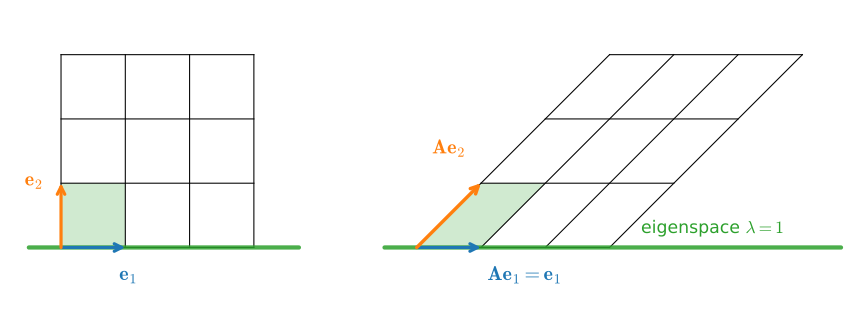
Its characteristic polynomial is \(\det(\mathbf{A}-\lambda\mathbf{I})=(1-\lambda)^2\), so \(\lambda=1\) has algebraic multiplicity \(2\). But solving \((\mathbf{A}-\mathbf{I})\mathbf{v}=\mathbf 0\) gives \(\bigl[\begin{smallmatrix}0&1\\0&0\end{smallmatrix}\bigr]\mathbf v=\mathbf 0\), i.e. \(v_2=0\): the eigenspace is the one-dimensional line spanned by \([1,0]^\top\). The geometric multiplicity is \(1\) while the algebraic multiplicity is \(2\), so there is no eigenbasis and \(\mathbf{A}\) is not diagonalizable; a matrix with this shortfall is called defective. Figure 24.2.2 makes the shortage visible: the shear slides every horizontal layer of the grid sideways, and the horizontal axis is the only line through the origin left pointing where it started. A diagonalizable \(2\times2\) matrix would exhibit two independent such lines; the shear has only one, and no change of basis can produce a second.
24.2.1.3.2 Beyond Diagonalization: The Jordan Normal Form
When the geometric multiplicity falls short of the algebraic multiplicity, no eigenbasis exists. What structure remains? The answer is completely catalogued. Over the complex numbers, every square matrix is similar to a block-diagonal matrix whose diagonal blocks are Jordan blocks
\[ \mathbf{J}_k(\lambda) = \begin{bmatrix} \lambda & 1 & & \\ & \lambda& \ddots & \\ & & \ddots & 1 \\ & & & \lambda \end{bmatrix}, \]
\(k\times k\) blocks with a single eigenvalue \(\lambda\) repeated down the diagonal and \(1\)s just above it. This is the Jordan normal form (Horn and Johnson 2012), which we use without proof.
The form makes both multiplicities visible at a glance, because each block contributes exactly one eigenvector: within a block, \((\mathbf{J}_k(\lambda)-\lambda\mathbf{I})\mathbf{v}=\mathbf 0\) forces every coordinate of \(\mathbf{v}\) except the first to vanish. So the geometric multiplicity of \(\lambda\) is the number of blocks carrying \(\lambda\), the algebraic multiplicity is the total size of those blocks, and a matrix is diagonalizable exactly when every block is \(1\times1\). The shear Equation 24.2.6 is already in Jordan form: it is the single block \(\mathbf{J}_2(1)\), one block of size two, hence one eigenvector for an eigenvalue of algebraic multiplicity two, exactly the shortage that Figure 24.2.2 displays.
What does a Jordan block do under iteration? Write \(\mathbf{J}_k(\lambda)=\lambda\mathbf{I}+\mathbf{N}\), where \(\mathbf{N}\) has \(1\)s just above the diagonal and zeros elsewhere. \(\mathbf{N}\) is a shift: it sends each basis vector to its predecessor, so \(\mathbf{N}^k=\mathbf 0\) (a matrix some power of which vanishes is called nilpotent). Because \(\mathbf{I}\) and \(\mathbf{N}\) commute, the binomial theorem applies to \((\lambda\mathbf{I}+\mathbf{N})^n\), and for \(k=2\) every term beyond the first two contains \(\mathbf{N}^2=\mathbf 0\):
\[ \mathbf{J}_2(\lambda)^n = (\lambda\mathbf{I}+\mathbf{N})^n = \lambda^n\mathbf{I} + n\lambda^{n-1}\mathbf{N}. \]
The eigenvalue still decides growth versus decay, but multiplied by a polynomial in \(n\) rather than acting alone. A defective matrix with \(|\lambda|=1\), like the shear, drifts linearly instead of staying put: \(\mathbf{J}_2(1)^n\) has an \(n\) in its corner. And with \(|\lambda|\) slightly below \(1\), the off-diagonal entry \(n\lambda^{n-1}\) first grows, peaks near \(n\approx-1/\log\lambda\), and only then decays: the iterates rise transiently before the geometric factor wins. We can watch this happen for \(\lambda=0.99\), where the formula puts the peak near \(n\approx100\).
J = np.array([[0.99, 1.], [0., 0.99]])   # the Jordan block J_2(0.99)
for n in [1, 50, 100, 200, 800]:
    Jn = np.linalg.matrix_power(J, n)
    pred = n * 0.99 ** (n - 1)   # predicted corner entry, n * lambda^(n-1)
    print(f'n = {n:3d}   ||J^n|| = {np.linalg.norm(Jn, 2):8.3f}   '
          f'n * 0.99^(n-1) = {pred:8.3f}')
n = 1 ||J^n|| = 1.609 n * 0.99^(n-1) = 1.000
n = 50 ||J^n|| = 30.568 n * 0.99^(n-1) = 30.556
n = 100 ||J^n|| = 36.977 n * 0.99^(n-1) = 36.973
n = 200 ||J^n|| = 27.067 n * 0.99^(n-1) = 27.067
n = 800 ||J^n|| = 0.260 n * 0.99^(n-1) = 0.260Every eigenvalue of \(\mathbf{J}\) is \(0.99\), safely below \(1\), yet the norm climbs to about \(37\) before the decay takes over. This transient growth is a signature of defective (more generally, non-normal) matrices, and it is invisible to the eigenvalues alone; the singular values of Section 24.3 measure it directly.
Jordan blocks are the first of two ways a real matrix can fall short of a real eigenbasis: too few eigenvectors. The second way is different in kind: a real matrix can have no real eigenvalue at all in some plane, because it rotates that plane.
24.2.1.3.3 Complex Eigenvalues Are Rotations
Consider the planar rotation by angle \(\theta\),
\[ \mathbf{R} = \begin{bmatrix}\cos\theta & -\sin\theta\\ \sin\theta & \phantom{-}\cos\theta\end{bmatrix}. \]
If \(0<\theta<\pi\), \(\mathbf{R}\) sends no nonzero real vector to a multiple of itself (a true rotation has no fixed direction), so it has no real eigenvector. Its characteristic polynomial \(\lambda^2-2\cos\theta\,\lambda+1\) has the complex-conjugate roots \(\lambda=\cos\theta\pm i\sin\theta=e^{\pm i\theta}\). The modulus \(|\lambda|=1\) records that \(\mathbf{R}\) preserves length (it is orthogonal), while the argument \(\pm\theta\) records the rotation angle.
theta = np.pi / 6
R = np.array([[np.cos(theta), -np.sin(theta)],
              [np.sin(theta),  np.cos(theta)]])
print('eigenvalues of R:', np.round(np.linalg.eigvals(R), 4))
print('expected e^{+/- i*theta}:', np.round(np.exp([1j * theta, -1j * theta]), 4))
print('moduli (should be 1):', np.round(np.abs(np.linalg.eigvals(R)), 4))
eigenvalues of R: [0.866+0.5j 0.866-0.5j]
expected e^{+/- i*theta}: [0.866+0.5j 0.866-0.5j]
moduli (should be 1): [1. 1.]This is the general rule. Complex eigenvalues of a real matrix come in conjugate pairs \(a\pm ib=re^{\pm i\theta}\), and each pair encodes a scale by \(r\) and rotate by \(\theta\) on some two-dimensional invariant plane. But where is that plane, and how do we pass between the complex pair and the real rotation? The dictionary is a two-line computation. Let \(\mathbf{A}\mathbf{w}=\lambda\mathbf{w}\) with \(\lambda=a+ib\), \(b\neq0\), and split the eigenvector into real and imaginary parts, \(\mathbf{w}=\mathbf{u}+i\mathbf{v}\). Expanding \(\mathbf{A}(\mathbf{u}+i\mathbf{v})=(a+ib)(\mathbf{u}+i\mathbf{v})\) and matching real and imaginary parts gives
\[ \mathbf{A}\mathbf{u} = a\mathbf{u} - b\mathbf{v}, \qquad \mathbf{A}\mathbf{v} = b\mathbf{u} + a\mathbf{v}. \]
Both images land back in \(\textrm{span}\{\mathbf{u},\mathbf{v}\}\), so this span is the invariant plane. (It really is a plane: if \(\mathbf{v}\) were a multiple of \(\mathbf{u}\), then \(\mathbf{u}\) would be a real eigenvector of \(\mathbf{A}\), forcing its eigenvalue to be real and contradicting \(b\neq0\).) Now collect the two identities into columns. With \(\mathbf{P}=[\mathbf{v}\;\;\mathbf{u}]\), they say exactly that \(\mathbf{A}\mathbf{P}=\mathbf{P}\left(\begin{smallmatrix}a & -b\\ b & \phantom{-}a\end{smallmatrix}\right)\), i.e.
\[ \mathbf{P}^{-1}\mathbf{A}\mathbf{P} = \begin{bmatrix} a & -b\\ b & \phantom{-}a \end{bmatrix} = \underbrace{\sqrt{a^2+b^2}}_{r}\, \begin{bmatrix} \cos\theta & -\sin\theta\\ \sin\theta & \phantom{-}\cos\theta \end{bmatrix}, \qquad \theta=\arg(a+ib). \tag{24.2.7}\]
In the basis \((\mathbf{v},\mathbf{u})\) of its invariant plane, \(\mathbf{A}\) is the rotation–scaling block: scale by the modulus, rotate by the argument. The dictionary also reads from right to left. Identify \((x,y)^\top\in\mathbb{R}^2\) with the complex number \(x+iy\); then the block acts as \((x,y)^\top\mapsto(ax-by,\,bx+ay)^\top\), which is precisely multiplication by \(a+ib\), and its eigenvalues are \(a\pm ib\) with eigenvectors \((1,\mp i)^\top\). Complex pair and real block carry the same two numbers in different coordinates, polar \((r,\theta)\) versus Cartesian \((a,b)\). Two conventions to keep straight: choosing the conjugate eigenvalue \(a-ib\) instead flips the sign of \(b\), giving the same plane traversed in the opposite orientation; and replacing \(\mathbf{w}\) by any nonzero complex multiple changes \(\mathbf{P}\) but not the block, since the derivation used only \(\mathbf{A}\mathbf{w}=\lambda\mathbf{w}\). So the block is well defined even though eig normalizes eigenvectors with an arbitrary phase. The following calculation verifies the dictionary on a matrix with no visible rotation.
A = np.array([[0.5, -1.2], [0.9, 0.3]])
lam, W = np.linalg.eig(A)
k = np.argmax(lam.imag)                  # the eigenvalue a + ib with b > 0
r, theta = np.abs(lam[k]), np.angle(lam[k])
u, v = W[:, k].real, W[:, k].imag
P = np.column_stack([v, u])              # basis (v, u) of the invariant plane
print(f'lambda = {lam[k]:.4f}   r = {r:.4f}   theta = {theta:.4f}')
print('P^-1 A P =\n', np.round(np.linalg.inv(P) @ A @ P, 4))
print('r * R(theta) =\n', np.round(r * np.array(
    [[np.cos(theta), -np.sin(theta)], [np.sin(theta), np.cos(theta)]]), 4))
lambda = 0.4000+1.0344j r = 1.1091 theta = 1.2018
P^-1 A P =
[[ 0.4 -1.0344]
[ 1.0344 0.4 ]]
r * R(theta) =
[[ 0.4 -1.0344]
[ 1.0344 0.4 ]]The entries of \(\mathbf{A}\) do not make the rotation apparent, yet in the basis read off from its eigenvector the map is exactly scale-by-\(r\), rotate-by-\(\theta\). Allowing such rotation–scaling blocks alongside the Jordan blocks of Section 24.2.1.3.2 gives the real Jordan form (Horn and Johnson 2012), and with it a complete inventory of what a linear map can do over the reals: every square matrix decomposes into pure stretch directions (real eigenvalues with a full set of eigenvectors), shear-like Jordan blocks (repeated eigenvalues with too few eigenvectors), and rotation–scaling planes (complex-conjugate pairs). The inventory also predicts how matrix iteration can behave: a dominant rotating pair keeps the iterate spinning forever instead of settling on a direction, and a dominant defective block converges with a polynomial drag. Both reappear when we develop power iteration later in this section. The dictionary itself returns in Section 29.1.2, where it converts eigenvalues into the phase portraits of continuous-time flows \(\dot{\mathbf{x}}=\mathbf{A}\mathbf{x}\): a complex pair \(a\pm ib\) produces a spiral, with the real part \(a\) setting growth or decay and the imaginary part \(b\) the angular velocity.
24.2.2 Non-Normal Matrices and Transient Amplification
The Jordan example showed that eigenvalues can miss a large temporary excursion. Defectiveness is the sharpest version of the problem, but it is not the whole problem: a matrix can have distinct eigenvalues, be diagonalizable, and still amplify some inputs substantially before its asymptotic decay becomes visible. Normality is the property that separates the clean case from this behavior.
24.2.2.1 Normality: When Eigenvalues Control Norms
Over the complex numbers, a matrix is normal when it commutes with its conjugate transpose,
\[ \mathbf A^*\mathbf A=\mathbf A\mathbf A^*. \]
For a real matrix, \(\mathbf A^*\) equals \(\mathbf A^\top\). Symmetric, orthogonal, and unitary matrices are normal, as are planar rotation–scaling blocks. The complex spectral theorem says that a matrix is normal if and only if it has an orthonormal eigenbasis over \(\mathbb C\): \(\mathbf A=\mathbf U\boldsymbol\Lambda\mathbf U^*\) with \(\mathbf U\) unitary. Consequently,
\[ \|\mathbf A^k\|_2 =\|\mathbf U\boldsymbol\Lambda^k\mathbf U^*\|_2 =\max_i|\lambda_i|^k =\rho(\mathbf A)^k. \tag{24.2.8}\]
For normal matrices the eigenvalues therefore control the largest possible amplification at every iteration, not merely its asymptotic exponential rate. This is why the orthonormal eigenbasis in the next section is more than an aesthetic convenience: the change of coordinates neither stretches nor nearly collapses any direction.
A diagonalizable non-normal matrix instead has \(\mathbf A=\mathbf W\boldsymbol\Lambda\mathbf W^{-1}\) with a generally non-orthogonal eigenvector matrix. The elementary bound
\[ \|\mathbf A^k\|_2 \le \underbrace{\|\mathbf W\|_2\|\mathbf W^{-1}\|_2}_{\kappa_2(\mathbf W)} \rho(\mathbf A)^k \tag{24.2.9}\]
exposes the missing factor: nearly parallel eigenvectors make \(\kappa_2(\mathbf W)\) large. Individual eigenmodes then carry large coefficients that can reinforce before their eventual cancellation. The bound need not be tight, but it explains why eigenvalues alone can be a poor finite-time diagnostic.
24.2.2.2 A Stable Matrix That First Grows
Consider the upper-triangular matrix
\[ \mathbf A=\begin{bmatrix}0.9&4\\0&0.8\end{bmatrix}. \tag{24.2.10}\]
Its distinct eigenvalues \(0.9\) and \(0.8\) make it diagonalizable, and both lie strictly inside the unit circle. Nevertheless, its eigenvectors are nearly parallel and its first few powers are large. The off-diagonal entry has the closed form
\[ (\mathbf A^k)_{12} =4\,\frac{0.9^k-0.8^k}{0.9-0.8} =40(0.9^k-0.8^k), \]
which initially grows even though both geometric factors decay. Singular values, rather than eigenvalue moduli, measure this one-step and finite-time stretch. The NumPy cell compares the non-normal matrix with the diagonal matrix having exactly the same eigenvalues.
A = np.array([[0.9, 4.0], [0.0, 0.8]])
D = np.diag([0.9, 0.8])                         # same eigenvalues, normal
ks = np.arange(0, 61)
norm_A = np.array([np.linalg.norm(np.linalg.matrix_power(A, k), 2) for k in ks])
norm_D = np.array([np.linalg.norm(np.linalg.matrix_power(D, k), 2) for k in ks])
k_peak = int(norm_A.argmax())
W = np.linalg.eig(A)[1]
z = 1.0
res_A = np.linalg.norm(np.linalg.inv(z * np.eye(2) - A), 2)
res_D = np.linalg.norm(np.linalg.inv(z * np.eye(2) - D), 2)
print('eigenvalues:', np.linalg.eigvals(A))
print(f'normal matrix: max ||D^k|| = {norm_D.max():.3f}')
print(f'non-normal:    max ||A^k|| = {norm_A[k_peak]:.3f} at k = {k_peak}')
print(f'eigenvector condition number = {np.linalg.cond(W):.1f}')
print(f'at z=1: ||(zI-A)^-1|| = {res_A:.1f},  normal comparison = {res_D:.1f}')
eigenvalues: [0.9 0.8]
normal matrix: max ||D^k|| = 1.000
non-normal: max ||A^k|| = 10.788 at k = 6
eigenvector condition number = 80.0
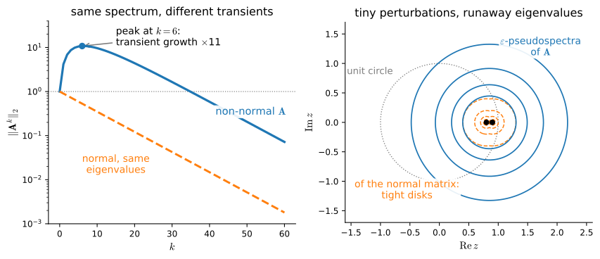
at z=1: ||(zI-A)^-1|| = 200.3, normal comparison = 10.0The normal matrix contracts from the first step. The non-normal matrix has the same spectral radius but amplifies a suitably chosen input by more than an order of magnitude before decay wins. This is transient amplification: stability as \(k\to\infty\) coexisting with substantial finite-time growth. Figure 24.2.3 compares the two cases. On a logarithmic scale, the norm curves eventually have the same slope, as implied by their common spectral radius. Before reaching that regime, the non-normal matrix amplifies its input by about a factor of ten, behavior not determined by its eigenvalues alone.
24.2.2.3 Pseudospectra: Stability under Perturbation
A second symptom of non-normality is eigenvalue sensitivity. For \(\varepsilon>0\), the \(\varepsilon\)-pseudospectrum is
\[ \Lambda_\varepsilon(\mathbf A) =\{z\in\mathbb C:\sigma_{\min}(z\mathbf I-\mathbf A)\le\varepsilon\} =\{z:z\text{ is an eigenvalue of }\mathbf A+\mathbf E \text{ for some }\|\mathbf E\|_2\le\varepsilon\}. \tag{24.2.11}\]
Away from an eigenvalue this can equivalently be read through the resolvent \((z\mathbf I-\mathbf A)^{-1}\): membership means its norm is at least \(1/\varepsilon\). For a normal matrix the resolvent norm is exactly the reciprocal distance from \(z\) to the nearest eigenvalue. For a non-normal matrix it can be much larger, so small perturbations can move eigenvalues far and a forced linear system can respond strongly even when \(z\) is not close to the displayed spectrum. The final line of the cell measures this effect at \(z=1\): the two matrices have the same eigenvalues, yet the non-normal resolvent is roughly twenty times larger. The right panel of Figure 24.2.3 draws the comparison whole — around the normal matrix’s eigenvalues the pseudospectral level sets are tight concentric disks, while around the non-normal matrix’s they balloon far beyond the unit circle at the same \(\varepsilon\).
Pseudospectra are primarily a diagnostic rather than another decomposition to memorize. In numerical linear algebra they warn that computed eigenvalues may be sensitive; in dynamical systems they warn about transient responses; and in deep learning they explain why a spectral-radius constraint alone does not control a layer’s Lipschitz constant or its gradient amplification.
24.2.2.4 Products of Jacobians
A recurrent or very deep network adds one complication: its backward map is a product of generally different Jacobians,
\[ \mathbf J_T\mathbf J_{T-1}\cdots\mathbf J_1. \]
Even if every factor has eigenvalues inside the unit circle, the factors need not share eigenvectors and their expanding singular directions can rotate into one another. The product’s norm therefore cannot be obtained by multiplying the factors’ spectral radii. Singular values give finite-horizon bounds, \(\|\mathbf J_T\cdots\mathbf J_1\|_2\le\prod_t\sigma_{\max}(\mathbf J_t)\); long-run average logarithmic growth is summarized by Lyapunov exponents. The practical hierarchy is now precise: eigenvalues describe asymptotic powers of one fixed map, singular values describe finite-time stretch, pseudospectra describe sensitivity, and Lyapunov exponents describe long products of changing maps.
24.2.3 Symmetric Matrices and Positive Definiteness
24.2.3.1 The Spectral Theorem
Shears and rotations tell us what can go wrong. We now restrict attention to the family of matrices for which a full set of orthonormal eigenvectors is guaranteed. The most commonly encountered are the symmetric matrices, those with \(\mathbf{A}=\mathbf{A}^\top\). Their guarantee has a name.
Theorem (Spectral Theorem). Every real symmetric matrix \(\mathbf{A}\) has a full orthonormal eigenbasis with real eigenvalues. Equivalently, \(\mathbf{A}=\mathbf{W}\boldsymbol{\Lambda}\mathbf{W}^\top\) where \(\boldsymbol{\Lambda}=\operatorname{diag}(\lambda_1,\ldots,\lambda_n)\) is real and \(\mathbf{W}\) is orthogonal (\(\mathbf{W}^\top\mathbf{W}=\mathbf{I}\), so \(\mathbf{W}^{-1}=\mathbf{W}^\top\)).
We prove the three claims in turn (real eigenvalues, orthogonal eigenvectors, and a complete basis); each proof is short and instructive. The inner product of complex vectors here is \(\langle\mathbf x,\mathbf y\rangle=\mathbf x^*\mathbf y\) with \(\mathbf x^*\) the conjugate transpose; on real vectors it is the ordinary dot product. The one fact we borrow is that a real polynomial, here the characteristic polynomial, has at least one (possibly complex) root, a special case of the fundamental theorem of algebra we invoked above, so at least one eigenpair exists over \(\mathbb{C}\).
Proof, part (i): the eigenvalues are real. Let \(\mathbf{A}\mathbf{v}=\lambda\mathbf{v}\) with \(\mathbf{v}\neq\mathbf 0\), allowing complex entries. Since \(\mathbf{A}\) is real and symmetric, \(\mathbf A^*=\mathbf A^\top=\mathbf A\), so
\[ \lambda\,\mathbf{v}^*\mathbf{v} = \mathbf{v}^*\mathbf{A}\mathbf{v} = (\mathbf{A}\mathbf{v})^*\mathbf{v} = \bar\lambda\,\mathbf{v}^*\mathbf{v}. \]
Because \(\mathbf{v}^*\mathbf{v}=\|\mathbf v\|^2>0\), we may divide it out to get \(\lambda=\bar\lambda\), i.e. \(\lambda\) is real. The eigenvector can then be taken real as well (it solves the real system \((\mathbf A-\lambda\mathbf I)\mathbf v=\mathbf0\)). \(\blacksquare\)
Proof, part (ii): eigenvectors for distinct eigenvalues are orthogonal. Let \(\mathbf{A}\mathbf{u}=\lambda\mathbf{u}\) and \(\mathbf{A}\mathbf{v}=\mu\mathbf{v}\) with \(\lambda\neq\mu\). Using \(\mathbf{A}=\mathbf{A}^\top\) to slide \(\mathbf{A}\) across the inner product,
\[ \lambda\langle\mathbf{u},\mathbf{v}\rangle = \langle\mathbf{A}\mathbf{u},\mathbf{v}\rangle = \langle\mathbf{u},\mathbf{A}\mathbf{v}\rangle = \mu\langle\mathbf{u},\mathbf{v}\rangle, \]
so \((\lambda-\mu)\langle\mathbf{u},\mathbf{v}\rangle=0\). Since \(\lambda\neq\mu\), we conclude \(\langle\mathbf{u},\mathbf{v}\rangle=0\): the eigenvectors are orthogonal. \(\blacksquare\)
Proof, part (iii): a full orthonormal basis (induction on the orthogonal complement). We induct on \(n\). For \(n=1\) the claim follows directly. For \(n>1\), part (i) gives a real eigenpair \((\lambda_1,\mathbf{w}_1)\) with \(\|\mathbf{w}_1\|=1\). Let \(U=\mathbf{w}_1^{\perp}\) be its orthogonal complement (dimension \(n-1\)). This subspace is \(\mathbf{A}\)-invariant: for any \(\mathbf{x}\in U\),
\[ \langle\mathbf{A}\mathbf{x},\mathbf{w}_1\rangle = \langle\mathbf{x},\mathbf{A}\mathbf{w}_1\rangle = \lambda_1\langle\mathbf{x},\mathbf{w}_1\rangle = 0, \]
so \(\mathbf{A}\mathbf{x}\in U\) too. The restriction \(\mathbf{A}|_U\) is again symmetric on an \((n-1)\)-dimensional space, so by the inductive hypothesis it has an orthonormal eigenbasis \(\mathbf{w}_2,\ldots,\mathbf{w}_n\) of \(U\). Together with \(\mathbf{w}_1\) these form an orthonormal eigenbasis of \(\mathbb{R}^n\). Collecting them as the columns of \(\mathbf{W}\) gives the stated factorization. \(\blacksquare\)
In this special case, then, we can write the eigendecomposition Equation 24.2.3 as
\[ \mathbf{A} = \mathbf{W}\boldsymbol{\Lambda}\mathbf{W}^\top . \tag{24.2.12}\]
This factorization is what makes PCA (the variance-maximizing projections of Section 24.3.2.2), covariance analysis, and the Hessian test for minima (Section 24.2.3.2) computable: all three concern symmetric matrices. It also reads geometrically: \(\mathbf{W}^\top\) rotates the orthonormal eigenvectors onto the coordinate axes, \(\boldsymbol{\Lambda}\) stretches independently along each axis, and \(\mathbf{W}\) rotates back. This is precisely the “circle becomes an ellipse with axes along the eigenvectors” picture we drew above, now justified.
The defective shear Equation 24.2.6 also shows the limits of eigendecomposition: it applies only to square matrices, and a general square matrix need not have an eigenbasis. The singular value decomposition avoids both restrictions by applying the spectral theorem to \(\mathbf{A}^\top\mathbf{A}\). This matrix is always symmetric (\((\mathbf A^\top\mathbf A)^\top=\mathbf A^\top\mathbf A\)) and positive semidefinite, because
\[ \mathbf{x}^\top(\mathbf{A}^\top\mathbf{A})\mathbf{x} = \|\mathbf{A}\mathbf{x}\|^2 \ge 0 . \]
The spectral theorem therefore applies to \(\mathbf{A}^\top\mathbf{A}\), and feeding its orthonormal eigenvectors and (non-negative) eigenvalues through \(\mathbf{A}\) yields the singular value decomposition \(\mathbf{A}=\mathbf{U}\boldsymbol{\Sigma}\mathbf{V}^\top\), with singular values \(\sigma_i=\sqrt{\lambda_i(\mathbf{A}^\top\mathbf{A})}\). We derive this construction and compute the SVD of the defective shear in Section 24.3. We first study positive semidefiniteness, the property that guarantees the eigenvalues are non-negative.
24.2.3.2 Positive (Semi)Definiteness
A symmetric matrix’s eigenvalues answer a sign question: is the quadratic form \(\mathbf{x}^\top\mathbf{A}\mathbf{x}\) ever negative? This one property is what makes covariance matrices, Gram matrices, and “is this a minimum?” Hessian tests work.
A symmetric matrix \(\mathbf{A}\) is positive semidefinite (PSD), written \(\mathbf{A}\succeq0\), if
\[ \mathbf{x}^\top\mathbf{A}\mathbf{x} \ge 0 \quad\textrm{for all } \mathbf{x}, \]
and positive definite (PD), written \(\mathbf{A}\succ0\), if the inequality is strict for every \(\mathbf{x}\neq\mathbf 0\). The eigenvalues decide the question completely.
Proposition (PSD/PD via eigenvalues). For symmetric \(\mathbf{A}\),
\[ \mathbf{A}\succeq0 \iff \lambda_i\ge0\ \forall i, \qquad \mathbf{A}\succ0 \iff \lambda_i>0\ \forall i . \]
Proof. Use the spectral theorem \(\mathbf{A}=\mathbf{W}\boldsymbol{\Lambda}\mathbf{W}^\top\) and the change of variables \(\mathbf{y}=\mathbf{W}^\top\mathbf{x}\). Since \(\mathbf{W}\) is orthogonal this is a rotation, and
\[ \mathbf{x}^\top\mathbf{A}\mathbf{x} = \mathbf{x}^\top\mathbf{W}\boldsymbol{\Lambda}\mathbf{W}^\top\mathbf{x} = \mathbf{y}^\top\boldsymbol{\Lambda}\mathbf{y} = \sum_{i=1}^{n}\lambda_i\,y_i^2 = \sum_{i=1}^{n}\lambda_i\,(\mathbf{w}_i^\top\mathbf{x})^2 . \tag{24.2.13}\]
The quadratic form is a weighted sum of squares with the eigenvalues as weights. If every \(\lambda_i\ge0\) the sum is \(\ge0\), so \(\mathbf{A}\succeq0\). Conversely, choosing \(\mathbf{x}=\mathbf{w}_j\) (so \(\mathbf y=\mathbf e_j\)) gives \(\mathbf{w}_j^\top\mathbf{A}\mathbf{w}_j=\lambda_j\), which forces \(\lambda_j\ge0\). The strict (PD) statement is identical with \(\ge\) replaced by \(>\). \(\blacksquare\)
Three consequences follow immediately, and together they cover most of the places PSD matrices appear in deep learning.
- PD \(\Rightarrow\) invertible. If \(\mathbf{A}\succ0\) and \(\mathbf{A}\mathbf{x}=\mathbf 0\), then \(\mathbf{x}^\top\mathbf{A}\mathbf{x}=0\), which forces \(\mathbf{x}=\mathbf 0\); the null space is trivial. (Equivalently, all \(\lambda_i>0\), so \(\det\mathbf A=\prod_i\lambda_i>0\) by Equation 24.2.4.)
- Gram and covariance matrices are PSD. For any matrix \(\mathbf{X}\), the Gram matrix \(\mathbf{G}=\mathbf{X}^\top\mathbf{X}\) satisfies \(\mathbf{x}^\top\mathbf{G}\mathbf{x}=\|\mathbf{X}\mathbf{x}\|^2\ge0\), so \(\mathbf{G}\succeq0\); it is PD exactly when \(\mathbf{X}\) has full column rank (so that \(\mathbf{X}\mathbf{x}=\mathbf 0\) implies \(\mathbf{x}=\mathbf 0\)). Covariance matrices, being Gram matrices of centered data divided by \(n\), inherit this: they are always PSD.
- The Hessian and minima. A twice-differentiable function has a local minimum at a critical point when its Hessian, the symmetric matrix \(\mathbf{H}\) of second partial derivatives \(h_{ij}=\partial^2 f/\partial x_i\partial x_j\) (developed in the calculus chapter), is PD there: by Equation 24.2.13 the second-order Taylor term \(\tfrac12\mathbf{x}^\top\mathbf{H}\mathbf{x}\) curves upward in every direction. This is the second-order optimality test we use throughout optimization.
Positive definiteness also has a purely algorithmic certificate, the Cholesky factorization: \(\mathbf{A}\succ0\) if and only if \(\mathbf{A}=\mathbf{L}\mathbf{L}^\top\) for a lower-triangular \(\mathbf{L}\) with positive diagonal (one direction is immediate: such an \(\mathbf{L}\) is invertible, so \(\mathbf{x}^\top\mathbf{A}\mathbf{x}=\|\mathbf{L}^\top\mathbf{x}\|^2>0\) for \(\mathbf{x}\neq\mathbf 0\)). Attempting the factorization is the standard numerical test for definiteness, and it is far cheaper than an eigendecomposition. The same factorization is how multivariate Gaussians are sampled, an application we develop in Section 27.2.
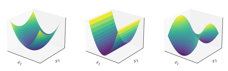
Geometrically, the sign pattern of the eigenvalues is the shape of the surface \(z=\mathbf{x}^\top\mathbf{A}\mathbf{x}\), viewed through the eigenvector axes: all-positive eigenvalues give an upward bowl (PD, a strict minimum at the origin), a zero eigenvalue gives a flat-bottomed trough along that eigenvector (PSD, not strict), and a mix of signs gives a saddle (indefinite). Figure 24.2.4 shows all three.
Let us verify the eigenvalue test against the definition numerically. We build a Gram matrix \(\mathbf{G}=\mathbf{X}^\top\mathbf{X}\) from a tall \(\mathbf{X}\) with full column rank (so it should be PD, all eigenvalues positive), and a second one whose columns are dependent (so it should be PSD with a zero eigenvalue).
X_full = np.array([[1., 0.], [1., 1.], [0., 1.], [2., 1.]])  # rank 2
X_dep = np.array([[1., 2.], [1., 2.], [0., 0.], [2., 4.]])   # col 2 = 2*col 1
for X, name in [(X_full, 'full column rank'), (X_dep, 'dependent columns')]:
    eigvals = np.linalg.eigvalsh(X.T @ X).round(4)
    eigvals[np.abs(eigvals) < 1e-9] = 0.0  # clean up tiny round-off / -0.0
    print(f'{name}: eigenvalues of X^T X = {eigvals}')
full column rank: eigenvalues of X^T X = [1.1459 7.8541]
dependent columns: eigenvalues of X^T X = [ 0. 30.]The full-rank case has both eigenvalues strictly positive (PD); the dependent case has a zero eigenvalue (PSD but not PD), exactly as the rank condition predicts.
24.2.3.3 The Rayleigh Quotient: Eigenvalues as Extreme Stretches
Identity Equation 24.2.13 does more than test signs: it pins down the largest and smallest eigenvalues as optimization problems. Define the Rayleigh quotient of a symmetric \(\mathbf{A}\),
\[ R(\mathbf{x}) = \frac{\mathbf{x}^\top\mathbf{A}\mathbf{x}}{\mathbf{x}^\top\mathbf{x}}, \qquad \mathbf{x}\neq\mathbf 0 . \]
Proposition (Rayleigh). For symmetric \(\mathbf{A}\) with eigenvalues \(\lambda_1\ge\cdots\ge\lambda_n\),
\[ \lambda_1 = \max_{\mathbf{x}\neq\mathbf 0} R(\mathbf{x}), \qquad \lambda_n = \min_{\mathbf{x}\neq\mathbf 0} R(\mathbf{x}), \]
attained at the corresponding eigenvectors.
Proof. Restrict to unit vectors (scaling \(\mathbf{x}\) leaves \(R\) unchanged). With \(\mathbf{y}=\mathbf{W}^\top\mathbf{x}\) we have \(\|\mathbf y\|=\|\mathbf x\|=1\) and, from Equation 24.2.13, \(\mathbf{x}^\top\mathbf{A}\mathbf{x}=\sum_i\lambda_i y_i^2\), a weighted average of the eigenvalues with non-negative weights \(y_i^2\) summing to \(1\). Any weighted average lies between the smallest and largest values, so \(\lambda_n\le R(\mathbf x)\le\lambda_1\); the bounds are achieved by putting all weight on a single coordinate, i.e. \(\mathbf x=\mathbf w_1\) or \(\mathbf x=\mathbf w_n\). \(\blacksquare\)
The following example sweeps a unit vector around the circle, records \(R(\mathbf{x})\) at each angle, and compares the extrema with the eigenvalues.
A = np.array([[3., 1.], [1., 2.]])
thetas = np.linspace(0, np.pi, 721)   # R has period pi: x and -x agree
xs = np.stack([np.cos(thetas), np.sin(thetas)])   # unit vectors, all angles
R = np.sum(xs * (A @ xs), axis=0)     # R(x) = x^T A x  (denominator is 1)
print(f'sweep of R:  min = {R.min():.6f}, max = {R.max():.6f}')
print(f'eigvalsh:    {np.linalg.eigvalsh(A).round(6)}')
sweep of R: min = 1.381967, max = 3.618033
eigvalsh: [1.381966 3.618034]The sweep never escapes the eigenvalue interval, and its extremes reproduce \(\lambda_{\min}\) and \(\lambda_{\max}\) to the resolution of the angular grid; the two angles where they occur are precisely the eigenvector directions. Every direction in between mixes the two eigenvalues in proportion to its squared eigen-coordinates, exactly as the weighted-average proof says.
Maximizing over subspaces of fixed dimension recovers every eigenvalue in between (the Courant–Fischer min-max theorem, \(\lambda_k=\max_{\dim S=k}\min_{\mathbf 0\neq\mathbf x\in S}R(\mathbf x)\)), though we will not need the general form. The Rayleigh quotient reappears in Section 24.3 as \(\sigma_1=\max_{\|\mathbf x\|=1}\|\mathbf{A}\mathbf x\|\) (the largest singular value) and as the variational characterization of PCA’s top component; in optimization, \(\lambda_{\max}(\mathbf H)\) is the worst-case curvature, the constant \(L\) that bounds a safe gradient-descent step size.
A large spread of Hessian eigenvalues means the PD bowl above is elongated, and gradient descent is slow on such a bowl. The ratio \(\kappa=\lambda_{\max}/\lambda_{\min}\) is the condition number, defined in general and analyzed in Section 24.3.3.2.
24.2.4 Localizing and Computing Eigenvalues
24.2.4.1 Gershgorin Discs
Eigenvalues are often difficult to reason with intuitively. If presented an arbitrary matrix, there is little that can be said about what the eigenvalues are without computing them. There is, however, one theorem that lets us localize them cheaply when the largest values are on the diagonal.
Theorem (Gershgorin (Gershgorin 1931)). Let \(\mathbf{A}=(a_{ij})\) be any \(n\times n\) matrix and let \(r_i=\sum_{j\neq i}|a_{ij}|\) be the off-diagonal absolute row sum. Let \(\mathcal{D}_i\) be the disc in the complex plane centered at \(a_{ii}\) with radius \(r_i\). Then every eigenvalue of \(\mathbf{A}\) lies in the union \(\bigcup_i\mathcal{D}_i\).
Proof. Let \(\mathbf{A}\mathbf{v}=\lambda\mathbf{v}\) with \(\mathbf{v}\neq\mathbf 0\), and pick the index \(i\) of the entry of largest magnitude, so \(|v_i|\ge|v_j|\) for all \(j\) (and \(v_i\neq0\)). Reading off row \(i\) of \(\mathbf{A}\mathbf{v}=\lambda\mathbf{v}\),
\[ \sum_j a_{ij}v_j = \lambda v_i \quad\Longrightarrow\quad (\lambda - a_{ii})\,v_i = \sum_{j\neq i} a_{ij} v_j . \]
Divide by \(v_i\) and take absolute values; since each \(|v_j/v_i|\le1\),
\[ |\lambda - a_{ii}| = \Bigl|\sum_{j\neq i} a_{ij}\,\tfrac{v_j}{v_i}\Bigr| \le \sum_{j\neq i} |a_{ij}| = r_i , \]
so \(\lambda\in\mathcal{D}_i\). \(\blacksquare\)
A useful corollary ties this section to the previous one. If \(\mathbf{A}\) is strictly diagonally dominant with positive diagonal (\(a_{ii}>r_i\) for every \(i\)), then every disc \(\mathcal D_i\) lives strictly in the right half-plane, so \(0\) is excluded from \(\bigcup_i\mathcal D_i\) and no eigenvalue can be zero. For a symmetric such matrix the eigenvalues are real and positive, so it is positive definite, hence invertible (Section 24.2.3.2). Localization thus gives a no-computation proof of invertibility, which is exactly the property one needs to guarantee numerical solvers will succeed.
Consider the matrix
\[ \mathbf{A} = \begin{bmatrix} 1.0 & 0.1 & 0.1 & 0.1 \\ 0.1 & 3.0 & 0.2 & 0.3 \\ 0.1 & 0.2 & 5.0 & 0.5 \\ 0.1 & 0.3 & 0.5 & 9.0 \end{bmatrix}. \]
We have \(r_1 = 0.3\), \(r_2 = 0.6\), \(r_3 = 0.8\) and \(r_4 = 0.9\). The matrix is symmetric, so all eigenvalues are real. This means that all of our eigenvalues will be in one of the ranges of
\[[a_{11}-r_1, a_{11}+r_1] = [0.7, 1.3], \tag{24.2.14}\]
\[[a_{22}-r_2, a_{22}+r_2] = [2.4, 3.6], \tag{24.2.15}\]
\[[a_{33}-r_3, a_{33}+r_3] = [4.2, 5.8], \tag{24.2.16}\]
\[[a_{44}-r_4, a_{44}+r_4] = [8.1, 9.9]. \tag{24.2.17}\]
Numerical computation gives eigenvalues of approximately \(0.99\), \(2.97\), \(4.95\), and \(9.08\), all comfortably inside the ranges provided.
import numpy as onp
A = onp.array([[1.0, 0.1, 0.1, 0.1],
              [0.1, 3.0, 0.2, 0.3],
              [0.1, 0.2, 5.0, 0.5],
              [0.1, 0.3, 0.5, 9.0]])

v, _ = onp.linalg.eig(A)
v
array([9.08033648, 0.99228545, 4.95394089, 2.97343718])The theorem is most vivid in a picture. Figure 24.2.5 draws the four discs in the complex plane and overlays the true eigenvalues, each one landing inside its disc.
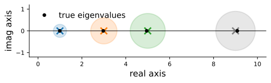
The discs localize the eigenvalues most tightly when the diagonal entries dominate the off-diagonal entries.
24.2.4.2 Power Iteration
We next use eigenvectors to analyze a simplified version of weight initialization in neural networks.
Complete initialization theory is beyond the scope of this chapter, so we consider a linear model. Neural networks alternate linear transformations and nonlinear operations. Here we omit the nonlinearities and repeatedly apply the matrix \(A\), written below as \(\mathbf{A}\), so that the output of our model is
\[ \mathbf{v}_{out} = \mathbf{A}\cdot \mathbf{A}\cdots \mathbf{A} \mathbf{v}_{in} = \mathbf{A}^N \mathbf{v}_{in}. \]
In a prediction problem, excessive growth under repeated application of \(\mathbf{A}\) amplifies small input perturbations, whereas excessive decay causes the output to lose dependence on the input. Repeatedly multiplying a random vector by \(\mathbf{A}\) and tracking its norm reveals that the ratio of consecutive norms stabilizes under the conditions below. The eigendecomposition identifies its limit.
Suppose \(\mathbf{A}\) is diagonalizable with a strictly dominant eigenvalue, \(|\lambda_1|>|\lambda_2|\ge\cdots\ge|\lambda_n|\), and eigenvectors \(\mathbf{w}_1,\ldots,\mathbf{w}_n\). We call \(\lambda_1\) the principal eigenvalue and \(\mathbf{w}_1\) the principal eigenvector. Expand the input in the eigenbasis, \(\mathbf{v}_0=\sum_i c_i\mathbf{w}_i\), and apply \(\mathbf{A}\) a total of \(k\) times. Because \(\mathbf{A}^k\mathbf{w}_i=\lambda_i^k\mathbf{w}_i\),
\[ \mathbf{A}^k\mathbf{v}_0 = \sum_{i=1}^{n} c_i\lambda_i^k\mathbf{w}_i = \lambda_1^k\Bigl(c_1\mathbf{w}_1 + \sum_{i\ge2} c_i\Bigl(\tfrac{\lambda_i}{\lambda_1}\Bigr)^{k}\mathbf{w}_i\Bigr). \tag{24.2.18}\]
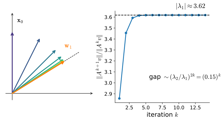
Every ratio \(|\lambda_i/\lambda_1|<1\), so as \(k\to\infty\) the bracket converges to \(c_1\mathbf{w}_1\): its tail decays to zero at the geometric rate \(|\lambda_2/\lambda_1|\), set by the slowest-decaying term. Provided \(c_1\neq0\) (the input has some component along \(\mathbf{w}_1\)), the iterate aligns with the principal eigenvector and its norm grows like \(|\lambda_1|^k\), so consecutive norms have ratio \(\to|\lambda_1|\). This is the classical power iteration for the dominant eigenpair (Golub and Van Loan 1996). Figure 24.2.6 makes the convergence concrete for the small symmetric matrix \(\mathbf{B}=[[3,1],[1,2]]\), which has a genuine strictly dominant real eigenvalue \(\lambda_1=(5+\sqrt5)/2\approx3.618\): the renormalized iterates swing onto \(\mathbf{w}_1\), their direction gap closing at the rate \(|\lambda_2/\lambda_1|=\tfrac{3-\sqrt5}{2}\approx0.382\), while the norm ratio flattens to \(\lambda_1\) even faster, at the squared rate \((\lambda_2/\lambda_1)^2\approx0.146\), because for a symmetric matrix the eigenvectors are orthogonal, so to first order the norm is insensitive to the remaining misalignment.
Two caveats, both places where the short version above would mislead. First, genericity: the argument needs \(c_1\neq0\), but a random Gaussian input has \(c_1=0\) with probability zero, so the method works almost surely. Second, strict dominance: when the two largest eigenvalues are a complex-conjugate pair of equal modulus, the dominant contribution rotates (see Section 24.2.1.3.3), and for a non-normal matrix the consecutive-norm ratio \(\|\mathbf{A}^{k+1}\mathbf{v}\|/\|\mathbf{A}^{k}\mathbf{v}\|\) can then oscillate forever, never converging. What always converges (for generic \(\mathbf{v}\)) is the averaged growth rate \(\|\mathbf{A}^{k}\mathbf{v}\|^{1/k}\to\max_i|\lambda_i|\). The random matrix in the demonstration below happens to draw a real, strictly dominant eigenvalue, so even the simple ratio settles.
The following numerical example runs 200 iterations on a random \(5\times5\) matrix and compares the stabilized norm ratio with the largest eigenvalue modulus.
import numpy as onp
onp.random.seed(8675309)
A = onp.random.randn(5, 5)
v = onp.random.randn(5, 1)
for _ in range(200):
    Av = A @ v
    ratio = onp.linalg.norm(Av) / onp.linalg.norm(v)
    v = Av / onp.linalg.norm(Av)
rho = max(abs(onp.linalg.eigvals(A)))
print(f'stabilized norm ratio = {ratio:.10f}   max|eigenvalue| = {rho:.10f}')
stabilized norm ratio = 1.9744593215 max|eigenvalue| = 1.9744593215The stabilized stretching factor matches the largest eigenvalue modulus to ten decimal places. One caveat: the random draw here happens to produce a real, strictly dominant eigenvalue, which is why the plain consecutive-norm ratio converges. Had the dominant eigenvalues been a complex pair, we would have read off the averaged rate \(\|\mathbf{A}^k\mathbf{v}\|^{1/k}\) instead, per the caveat above. Either way, the quantity being measured has a name: the spectral radius \(\rho(\mathbf A)=\max_i|\lambda_i|\), the largest eigenvalue modulus, which we examine next.
24.2.4.2.1 Aside: PageRank and the Perron–Frobenius Theorem
For non-negative matrices, power iteration is also the algorithm of choice for computing the dominant eigenvector, and that eigenvector is often the target. The Perron–Frobenius theorem (Horn and Johnson 2012) says that a matrix with non-negative entries (and a mild connectivity condition, irreducibility: from every state you can reach every other) has a real, positive dominant eigenvalue whose eigenvector can be chosen with all entries non-negative, so it is interpretable as a distribution. Google’s original PageRank (Brin and Page 1998) is exactly this eigenvector. Model a random web surfer who at each step follows a random outgoing link. Before forming a transition matrix, repair every dangling page (one with no outgoing links), for example by replacing its empty column by the uniform distribution. The resulting click probabilities form a column-stochastic matrix \(\mathbf{P}\) (every column sums to \(1\), and every entry is non-negative). Two lines show that \(\rho(\mathbf{P})=1\). Because the columns sum to one, \(\mathbf{1}^\top\mathbf{P}=\mathbf{1}^\top\), so \(1\) is an eigenvalue of \(\mathbf{P}^\top\) and hence of \(\mathbf{P}\) (a matrix and its transpose share the characteristic polynomial, since \(\det(\mathbf{M}^\top)=\det(\mathbf{M})\)). And no eigenvalue can exceed modulus \(1\): applying the Gershgorin theorem of Section 24.2.4.1 to \(\mathbf{P}^\top\), whose rows are the columns of \(\mathbf{P}\), puts every eigenvalue in a disc centered at \(p_{ii}\ge0\) with radius \(1-p_{ii}\), hence within modulus \(p_{ii}+(1-p_{ii})=1\). The fraction of time the surfer spends on each page is the stationary distribution \(\boldsymbol\pi\) with \(\mathbf{P}\boldsymbol\pi=\boldsymbol\pi\), the dominant eigenvector. One wrinkle: the repaired link matrix can still fail irreducibility or be periodic because the web contains disconnected pockets and cycles. The separate fix is damping: iterate the blended matrix \(\alpha\mathbf{P}+(1-\alpha)\tfrac1n\mathbf{1}\mathbf{1}^\top\) with \(\alpha\approx0.85\), i.e. with probability \(0.15\) the surfer teleports to a uniformly random page. Every entry of the blend is positive, so Perron–Frobenius applies by construction, and it guarantees the gap \(|\lambda_2|\le\alpha\) (Haveliwala and Kamvar 2003), so power iteration converges fast. Power iteration started from the uniform distribution converges to \(\boldsymbol\pi\), and that is precisely how PageRank is computed at web scale: forming \(\mathbf{P}\) explicitly is unthinkable, but multiplying by it is cheap (and the teleportation term is rank one, so the damped multiply costs no more). The same dominant-eigenvector-by-power-iteration idea reappears across machine learning, in the stationary distribution of a Markov chain and in spectral clustering.
24.2.5 Spectral Radius, Stability, and Deep Networks
The spectral radius \(\rho(\mathbf A)=\max_i|\lambda_i|\) controls the asymptotic exponential rate of powers of one fixed matrix:
\[ \lim_{k\to\infty}\|\mathbf A^k\|^{1/k}=\rho(\mathbf A). \]
This statement is weaker than saying that \(\|\mathbf A^k\|\) is approximately \(\rho(\mathbf A)^k\) at every finite \(k\). A defective Jordan block contributes polynomial factors, and a non-normal matrix can amplify some vectors greatly before its eventual asymptotic behavior takes over. For example, \(\mathbf A=\left[\begin{smallmatrix}1&1\\0&1\end{smallmatrix}\right]\) has \(\rho(\mathbf A)=1\) but \(\mathbf A^k=\left[\begin{smallmatrix}1&k\\0&1\end{smallmatrix}\right]\). Thus rescaling to \(\rho(\mathbf A)=1\) controls the exponential rate but does not guarantee bounded iterates. This distinction matters for initialization and raises the question of how large \(\rho\) typically is to begin with.
24.2.5.1 What Random Matrices Look Like
Random matrix theory answers it. The real Ginibre ensemble (Ginibre 1965) is the \(n\times n\) matrix whose entries are independent with mean zero and variance one. For this ensemble the rescaled eigenvalues \(\lambda_i/\sqrt n\) fill the unit disk in the complex plane roughly uniformly as \(n\to\infty\): the circular law (Tao and Vu 2010). Consequently \(\rho(\mathbf A)/\sqrt n\to1\): the spectral radius grows like \(\sqrt n\), with the largest modulus sitting just outside the bulk of the disk. At finite \(n\) this is only a tendency (for the small \(5\times5\) example above we should not expect to land exactly on \(\sqrt5\approx2.24\), since finite-size fluctuations are substantial), but the scaling with \(\sqrt n\) is what matters for initialization: it is why sensible schemes scale random weights by \(1/\sqrt n\) (equivalently, by \(1/\sqrt{\textrm{fan-in}}\)) to keep \(\rho\) near \(1\).
A word of caution: the spectral radius is not the same as the largest singular value of such a matrix, which by the Marchenko–Pastur law sits near \(2\sqrt{n}\) at finite \(n\). We return to singular values, and to the deeper connections between random-matrix spectra and initialization (Pennington et al. 2017), in Section 24.3.
Symmetric random matrices have their own law, and it is the one a data analyst meets first. Take \(n\) samples of a \(d\)-dimensional vector with independent, mean-zero, unit-variance coordinates (pure noise, true covariance \(\mathbf{I}\)) and form the sample covariance \(\hat{\boldsymbol\Sigma}=\tfrac1n\mathbf{X}^\top\mathbf{X}\). The relevant parameter is the aspect ratio \(\gamma=d/n\), the number of dimensions each sample must account for. One might hope the eigenvalues all sit near \(1\). They spread instead: for \(\gamma\) held fixed, they cover the Marchenko–Pastur bulk \([(1-\sqrt\gamma)^2,\,(1+\sqrt\gamma)^2]\) (Marchenko and Pastur 1967); with \(d=n/4\) the “noise” eigenvalues range across \([0.25, 2.25]\). This bulk is the null hypothesis of spectral data analysis: an eigenvalue inside it is indistinguishable from sampling noise, and only eigenvalues that escape above the bulk edge testify to real structure (the calibration behind the singular-value threshold of Section 24.3.2.1). It is also the baseline for the heavy-tailed spectra of trained weight matrices, which spill far outside any Marchenko–Pastur bulk; Section 24.3 reads that excess as evidence of learned correlation.
The iterated map is exactly what a recurrent network runs. It computes a hidden state \(\mathbf{h}_t=\phi(\mathbf{W}\mathbf{h}_{t-1}+\cdots)\) by applying (almost) the same transformation at every time step, and backpropagation through time multiplies the per-step Jacobians:
\[ \nabla_{\mathbf{h}_0}\mathcal{L} = \mathbf{J}_1^\top\mathbf{J}_2^\top\cdots\mathbf{J}_T^\top \,\nabla_{\mathbf{h}_T}\mathcal{L}, \qquad \mathbf{J}_t=\frac{\partial\mathbf{h}_t}{\partial\mathbf{h}_{t-1}} . \]
This is a product of matrices applied to a vector. In the idealized linear case where every Jacobian is the same diagonalizable matrix \(\mathbf J\), its asymptotic exponential rate is governed by \(\rho(\mathbf J)\). Actual recurrent networks multiply different, generally non-normal Jacobians. Their gradient norm is controlled directly by singular values of the product \(\mathbf J_T\cdots\mathbf J_1\), or asymptotically by Lyapunov exponents; the spectral radii of the individual factors do not determine it. Large singular values can produce exploding gradients and small ones vanishing gradients (Bengio et al. 1994; Pascanu et al. 2013).
This refined view explains why orthogonal/identity initialization (Saxe et al. 2014), gradient clipping, and the gating mechanisms of LSTMs and GRUs help: they control finite-time amplification and information flow, not merely eigenvalue moduli. Singular values and condition numbers, introduced in Section 24.3, supply the right single-layer language; products require the same ideas applied along the whole trajectory.
24.2.6 Summary
- Eigenvectors are directions a matrix stretches without rotating; eigenvalues are the stretch factors. The unit circle maps to an ellipse whose axes, for a symmetric matrix, lie along the eigenvectors with half-lengths \(|\lambda_i|\).
- A matrix is diagonalizable (\(\mathbf{A}=\mathbf{W}\boldsymbol{\Lambda}\mathbf{W}^{-1}\)) exactly when its eigenvectors span the space, i.e. geometric multiplicity equals algebraic multiplicity for every eigenvalue; \(n\) distinct eigenvalues guarantee it.
- The eigenvalues reduce many operations to scalar ones: \(\mathbf{A}^n\) raises them to the \(n\), and because determinant is multiplicative and trace is cyclic, similarity invariance gives \(\det\mathbf{A}=\prod_i\lambda_i\) and \(\operatorname{tr}\mathbf{A}=\sum_i\lambda_i\).
- Over the reals, every square matrix decomposes into pure stretch directions, shear-like Jordan blocks (defective eigenvalues), and rotation–scaling planes (complex-conjugate pairs). A Jordan block grows like \(\lambda^n\) times a polynomial in \(n\), so a defective matrix can grow transiently even when every \(|\lambda_i|<1\).
- The spectral theorem guarantees real symmetric matrices an orthonormal eigenbasis with real eigenvalues, \(\mathbf{A}=\mathbf{W}\boldsymbol{\Lambda}\mathbf{W}^\top\); applied to \(\mathbf{A}^\top\mathbf{A}\) it builds the SVD for every matrix.
- Positive (semi)definiteness is decided by the sign of the eigenvalues, via \(\mathbf{x}^\top\mathbf{A}\mathbf{x}=\sum_i\lambda_i(\mathbf{w}_i^\top\mathbf{x})^2\); this governs Gram/covariance matrices and the Hessian minimum test. The Rayleigh quotient identifies \(\lambda_{\max}\) and \(\lambda_{\min}\) as extreme stretches.
- The Gershgorin Circle Theorem localizes the eigenvalues in discs around the diagonal, giving cheap bounds and a no-computation invertibility test.
- The spectral radius gives the asymptotic exponential rate of powers of one fixed matrix, but Jordan blocks and non-normality can cause polynomial or transient growth. Recurrent gradients involve products of changing Jacobians, so their singular values and Lyapunov exponents, rather than the factors’ spectral radii alone, control exploding and vanishing gradients.
24.2.7 Exercises
- For the non-normal matrix in Equation 24.2.10, derive the formula for \((\mathbf A^k)_{12}\) by diagonalization or induction. Find the integer \(k\) at which this entry is largest, and compare it with the NumPy result for \(\|\mathbf A^k\|_2\).
- Prove Equation 24.2.8 from a unitary diagonalization. Then construct a diagonalizable \(2\times2\) matrix with spectral radius \(1/2\) but one-step norm larger than an arbitrary prescribed \(M>0\).
- What are the eigenvalues and eigenvectors of \[ \mathbf{A} = \begin{bmatrix} 2 & 1 \\ 1 & 2 \end{bmatrix}? \]
- What are the eigenvalues and eigenvectors of the following matrix, and what is strange about this example compared to the previous one? \[ \mathbf{A} = \begin{bmatrix} 2 & 1 \\ 0 & 2 \end{bmatrix}. \]
- Without computing the eigenvalues, determine whether the smallest eigenvalue of the following matrix can be less than \(0.5\). Use a bound rather than explicit computation. \[ \mathbf{A} = \begin{bmatrix} 3.0 & 0.1 & 0.3 & 1.0 \\ 0.1 & 1.0 & 0.1 & 0.2 \\ 0.3 & 0.1 & 5.0 & 0.0 \\ 1.0 & 0.2 & 0.0 & 1.8 \end{bmatrix}. \]
- Classify each matrix as positive definite, positive semidefinite, or indefinite from its eigenvalues: \(\begin{bmatrix}2&1\\1&2\end{bmatrix}\), \(\begin{bmatrix}1&2\\2&1\end{bmatrix}\), and \(\begin{bmatrix}1&1\\1&1\end{bmatrix}\).
- Prove that for any matrix \(\mathbf{X}\), the Gram matrix \(\mathbf{X}^\top\mathbf{X}\) is positive semidefinite, and is positive definite if and only if \(\mathbf{X}\) has full column rank. Conclude that the sum of two positive semidefinite matrices is again positive semidefinite.
- Using \(\det\mathbf{A}=\prod_i\lambda_i\) and \(\operatorname{tr}\mathbf{A}=\sum_i\lambda_i\), find both eigenvalues of \(\begin{bmatrix}4&1\\1&4\end{bmatrix}\) without forming the characteristic polynomial directly. (Hint: their sum and product are known.)
- Verify the Rayleigh-quotient bounds for \(\mathbf{A}=\begin{bmatrix}3&1\\1&2\end{bmatrix}\): compute \(\mathbf{x}^\top\mathbf{A}\mathbf{x}/\mathbf{x}^\top\mathbf{x}\) for several unit vectors and confirm the values stay between \(\lambda_{\min}\) and \(\lambda_{\max}\), hitting the endpoints at the eigenvectors.
- The power-iteration tail in Equation 24.2.18 decays at rate \(|\lambda_2/\lambda_1|\). For \(\mathbf{B}=\begin{bmatrix}3&1\\1&2\end{bmatrix}\), compute this rate and predict roughly how many iterations are needed to reduce the misalignment by a factor of \(100\).
- Compute \(\mathbf{J}_2(\lambda)^n\) by hand by writing \(\mathbf{J}_2(\lambda)=\lambda\mathbf{I}+\mathbf{N}\) and using \(\mathbf{N}^2=\mathbf{0}\). For \(\lambda=0.99\), at which \(n\) does \(\|\mathbf{J}_2(\lambda)^n\|\) peak? Check your prediction against the code in Section 24.2.1.3.2.