%matplotlib inline
from d2l import torch as d2l
import torch
from torch import nn2.7 Weight Decay
Now that we have characterized the problem of overfitting, we can introduce our first regularization technique. Additional representative training data often reduces overfitting. However, that can be costly, time consuming, or entirely out of our control, making it impossible in the short run. For now, we can assume that we already have as much high-quality data as our resources permit and focus on the tools at our disposal when the dataset is taken as a given.
Recall that in our polynomial regression example (Section 2.6.2.1) we could limit our model’s capacity by tweaking the degree of the fitted polynomial. Indeed, limiting the number of features is a popular technique for mitigating overfitting. However, discarding features can be too coarse a way to control capacity. Sticking with the polynomial regression example, consider what might happen with high-dimensional input. The natural extensions of polynomials to multivariate data are called monomials, which are products of powers of variables. The degree of a monomial is the sum of the powers. For example, \(x_1^2 x_2\), and \(x_3 x_5^2\) are both monomials of degree 3.
The number of terms with degree \(d\) grows rapidly with \(d\). Given \(k\) variables, the number of monomials of degree \(d\) is \(\binom{k-1+d}{k-1}\). Even small changes in degree, say from \(2\) to \(3\), dramatically increase the complexity of our model. Thus we often need a more fine-grained tool for adjusting function complexity.
%matplotlib inline
from d2l import tensorflow as d2l
import tensorflow as tf%matplotlib inline
from d2l import jax as d2l
import jax
from jax import numpy as jnp
import optax%matplotlib inline
from d2l import mxnet as d2l
from mxnet import autograd, gluon, init, np, npx
from mxnet.gluon import nn
npx.set_np()2.7.1 Norms and Weight Decay
Rather than directly manipulating the number of parameters, weight decay (Hanson and Pratt 1988; Krogh and Hertz 1992) operates by restricting the values that the parameters can take. Outside of deep learning circles the technique is better known as \(\ell_2\) regularization (the two coincide when optimizing by minibatch SGD, a point we return to below), and it is a widely used regularizer for parametric machine learning models. The technique is motivated by the basic intuition that, within a fixed parameterization, a function \(f\) with smaller parameter norm has lower penalty. This expresses a preference toward the zero function \(f = 0\), which assigns \(0\) to every input. The choice of norm determines how parameter size is measured. There is no single right answer. In fact, entire branches of mathematics, including parts of functional analysis and the theory of Banach spaces, are devoted to addressing such issues.
One simple interpretation might be to measure the complexity of a linear function \(f(\mathbf{x}) = \mathbf{w}^\top \mathbf{x}\) by some norm of its weight vector, e.g., \(\| \mathbf{w} \|^2\). Recall that we introduced the \(\ell_2\) norm and \(\ell_1\) norm, which are special cases of the more general \(\ell_p\) norm, in Section 1.3.4. The most common method for ensuring a small weight vector is to add its norm as a penalty term to the problem of minimizing the loss. Thus we replace our original objective, minimizing the prediction loss on the training labels, with a new objective, minimizing the sum of the prediction loss and the penalty term. Now, if our weight vector grows too large, our learning algorithm might focus on minimizing the weight norm \(\| \mathbf{w} \|^2\) rather than minimizing the training error. That is exactly what we want. To illustrate things in code, we revive our previous example from Section 2.1 for linear regression. There, our loss was given by
\[L(\mathbf{w}, b) = \frac{1}{n}\sum_{i=1}^n \frac{1}{2}\left(\mathbf{w}^\top \mathbf{x}^{(i)} + b - y^{(i)}\right)^2. \tag{2.7.1}\]
Recall that \(\mathbf{x}^{(i)}\) are the features, \(y^{(i)}\) is the label for any data example \(i\), and \((\mathbf{w}, b)\) are the weight and bias parameters, respectively. To penalize the size of the weight vector, we must somehow add \(\| \mathbf{w} \|^2\) to the loss function, but how should the model trade off the standard loss for this new additive penalty? In practice, we characterize this trade-off via the regularization constant \(\lambda\), a nonnegative hyperparameter that we fit using validation data:
\[L(\mathbf{w}, b) + \frac{\lambda}{2} \|\mathbf{w}\|^2. \tag{2.7.2}\]
For \(\lambda = 0\), we recover our original loss function. For \(\lambda > 0\), we restrict the size of \(\| \mathbf{w} \|\). We divide by \(2\) by convention: when we take the derivative of a quadratic function, the \(2\) and \(1/2\) cancel out, ensuring that the expression for the update looks nice and simple. We use the squared norm rather than the norm itself for computational convenience. By squaring the \(\ell_2\) norm, we remove the square root, leaving the sum of squares of each component of the weight vector. This makes the derivative of the penalty easy to compute: the sum of derivatives equals the derivative of the sum.
Other penalties are also valid and popular throughout statistics. While \(\ell_2\)-regularized linear models constitute the classic ridge regression algorithm (Hoerl and Kennard 1970), \(\ell_1\)-regularized linear regression is a similarly fundamental method in statistics, popularly known as lasso regression (Tibshirani 1996). One reason to work with the \(\ell_2\) norm is that it places an outsize penalty on large components of the weight vector. This biases our learning algorithm towards models that distribute weight evenly across a larger number of features. In practice, this might make them more robust to measurement error in a single variable. By contrast, \(\ell_1\) penalties lead to models that concentrate weights on a small set of features by clearing the other weights to zero. This gives us an effective method for feature selection, which may be desirable for other reasons. For example, if our model only relies on a few features, then we may not need to collect, store, or transmit data for the other (dropped) features.
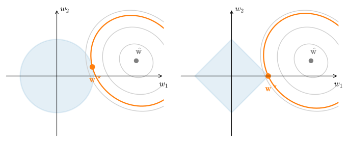
These two penalties are easiest to compare geometrically. For a corresponding budget \(t\), minimizing \(L(\mathbf{w}) + \frac{\lambda}{2}\|\mathbf{w}\|^2\) is equivalent to minimizing \(L(\mathbf{w})\) subject to \(\|\mathbf{w}\| \le t\), and the regularized solution is the first point at which a loss contour meets the constraint region (Figure 2.7.1). A smooth \(\ell_2\) boundary usually shrinks coordinates without making them exactly zero. The corners and faces of the \(\ell_1\) ball make exact zeros much more common, although sparsity is not guaranteed for every loss and dataset. This geometry explains why lasso can perform feature selection while ridge usually does not. We assert the penalty\(\,\Leftrightarrow\,\)constraint equivalence here; Section 26.4 derives it via Lagrange duality (\(\lambda\) is exactly the multiplier attached to the constraint \(\|\mathbf{w}\| \le t\)) and computes the \(\lambda \leftrightarrow t\) correspondence numerically on ridge regression.
Using the same notation as in Equation 2.1.9, the minibatch stochastic gradient descent update for \(\ell_2\)-regularized regression is as follows:
\[\begin{aligned} \mathbf{w} & \leftarrow \left(1- \eta\lambda \right) \mathbf{w} - \frac{\eta}{|\mathcal{B}|} \sum_{i \in \mathcal{B}} \mathbf{x}^{(i)} \left(\mathbf{w}^\top \mathbf{x}^{(i)} + b - y^{(i)}\right). \end{aligned} \tag{2.7.3}\]
As before, we update \(\mathbf{w}\) based on the amount by which our estimate differs from the observation. However, we also shrink the size of \(\mathbf{w}\) towards zero. That is why the method is sometimes called “weight decay”: given the penalty term alone, our optimization algorithm decays the weight at each step of training. In contrast to feature selection, weight decay offers us a mechanism for continuously adjusting the complexity of a function. Smaller values of \(\lambda\) correspond to less constrained \(\mathbf{w}\), whereas larger values of \(\lambda\) constrain \(\mathbf{w}\) more considerably. Whether we include a corresponding bias penalty \(b^2\) can vary across implementations, and may vary across layers of a neural network. Often, we do not regularize the bias term. For plain minibatch stochastic gradient descent, adding \(\frac{\lambda}{2}\|\mathbf{w}\|^2\) to the loss and applying the shrink-and-update rule above are one and the same. This equivalence is special to SGD: for adaptive optimizers such as Adam, a penalty placed inside the loss is rescaled by the optimizer’s per-coordinate second-moment estimates and no longer acts as uniform weight shrinkage. Decoupling the decay from the loss gradient restores the intended behavior, shrinking every weight by a fixed fraction at each step; this is the decoupled-weight-decay variant AdamW, introduced by Loshchilov and Hutter (2019) and now a default optimizer for large models. The mechanism (including the per-coordinate shrinkage formula and a code demonstration racing the coupled and decoupled variants) is worked out in Section 26.2.3, and we take up optimizers in detail in Section 9.6.
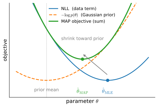
Finally, weight decay also has a probabilistic reading. Recall from Section 2.1.3 that minimizing the squared loss is maximum likelihood estimation under Gaussian observation noise. Now place an isotropic Gaussian prior \(\mathbf{w} \sim \mathcal{N}(\mathbf{0}, \tau^2\mathbf{I})\) on the weights and ask instead for the weights that maximize the posterior \(p(\mathbf{w} \mid \mathbf{X}, \mathbf{y}) \propto p(\mathbf{y} \mid \mathbf{X}, \mathbf{w})\, p(\mathbf{w})\), the maximum a posteriori (MAP) estimate. Taking negative logarithms, the prior contributes
\[-\log p(\mathbf{w}) = \frac{1}{2\tau^2} \|\mathbf{w}\|^2 + \textrm{const}, \tag{2.7.4}\]
so the MAP objective is the Gaussian negative log-likelihood of Section 2.1.3 plus a quadratic penalty:
\[-\log p(\mathbf{w} \mid \mathbf{X}, \mathbf{y}) = \frac{1}{2\sigma^2} \sum_{i=1}^n \left(y^{(i)} - \mathbf{w}^\top \mathbf{x}^{(i)} - b\right)^2 + \frac{1}{2\tau^2} \|\mathbf{w}\|^2 + \textrm{const}. \tag{2.7.5}\]
In short, MAP estimation is maximum likelihood plus a prior, and the objective above is exactly of our weight-decay form. The regularization constant \(\lambda\) is thereby proportional to the prior precision \(1/\tau^2\): a tighter prior (smaller \(\tau\)) means stronger shrinkage. Because \(L\) is the average half-squared error while the log-posterior contains a sum, multiplying the negative log-posterior by \(\sigma^2/n\) gives
\[L(\mathbf{w},b)+\frac{\lambda}{2}\|\mathbf{w}\|^2, \qquad \lambda=\frac{\sigma^2}{n\tau^2}. \tag{2.7.6}\]
Thus regularization strength depends on prior precision, observation noise, and sample size under this averaging convention. Figure 2.7.2 illustrates this: the quadratic prior shifts the maximum-likelihood estimate toward the origin. This recovers the classical ridge regression estimator.
2.7.2 High-Dimensional Linear Regression
A synthetic example illustrates the effect of weight decay.
First, we generate some data as before:
\[y = 0.05 + \sum_{i = 1}^d 0.01 x_i + \epsilon \textrm{ where } \epsilon \sim \mathcal{N}(0, 0.01^2). \tag{2.7.7}\]
In this synthetic dataset, our label is given by an underlying linear function of our inputs, corrupted by Gaussian noise with zero mean and standard deviation 0.01. To make overfitting visible, we increase the dimensionality of our problem to \(d = 200\) and working with a small training set with only 20 examples.
class Data(d2l.DataModule):
    def __init__(self, num_train, num_val, num_inputs, batch_size):
        self.save_hyperparameters()
        n = num_train + num_val
        self.X = d2l.randn(n, num_inputs)
        noise = d2l.randn(n, 1) * 0.01
        w, b = d2l.ones((num_inputs, 1)) * 0.01, 0.05
        self.y = d2l.matmul(self.X, w) + b + noise

    def get_dataloader(self, train):
        i = slice(0, self.num_train) if train else slice(self.num_train, None)
        return self.get_tensorloader([self.X, self.y], train, i)
class Data(d2l.DataModule):
def __init__(self, num_train, num_val, num_inputs, batch_size):
self.save_hyperparameters()
n = num_train + num_val
self.X = d2l.normal((n, num_inputs))
noise = d2l.normal((n, 1)) * 0.01
w, b = d2l.ones((num_inputs, 1)) * 0.01, 0.05
self.y = d2l.matmul(self.X, w) + b + noise
def get_dataloader(self, train):
i = slice(0, self.num_train) if train else slice(self.num_train, None)
return self.get_tensorloader([self.X, self.y], train, i)class Data(d2l.DataModule):
def __init__(self, num_train, num_val, num_inputs, batch_size):
self.save_hyperparameters()
n = num_train + num_val
key_X, key_noise = jax.random.split(jax.random.key(0))
self.X = jax.random.normal(key_X, (n, num_inputs))
noise = jax.random.normal(key_noise, (n, 1)) * 0.01
w, b = d2l.ones((num_inputs, 1)) * 0.01, 0.05
self.y = d2l.matmul(self.X, w) + b + noise
def get_dataloader(self, train):
i = slice(0, self.num_train) if train else slice(self.num_train, None)
return self.get_tensorloader([self.X, self.y], train, i)class Data(d2l.DataModule):
def __init__(self, num_train, num_val, num_inputs, batch_size):
self.save_hyperparameters()
n = num_train + num_val
self.X = d2l.randn(n, num_inputs)
noise = d2l.randn(n, 1) * 0.01
w, b = d2l.ones((num_inputs, 1)) * 0.01, 0.05
self.y = d2l.matmul(self.X, w) + b + noise
def get_dataloader(self, train):
i = slice(0, self.num_train) if train else slice(self.num_train, None)
return self.get_tensorloader([self.X, self.y], train, i)2.7.3 Implementation from Scratch
We first implement weight decay from scratch. Since minibatch stochastic gradient descent is our optimizer, we just need to add the squared \(\ell_2\) penalty to the original loss function.
2.7.3.1 Defining \(\ell_2\) Norm Penalty
Perhaps the most convenient way of implementing this penalty is to square all terms in place and sum them.
def l2_penalty(w):
    return d2l.reduce_sum(w**2) / 2
2.7.3.2 Defining the Model
In the final model, the linear regression and the squared loss have not changed since Section 2.4, so we will just define a subclass of d2l.LinearRegressionScratch. The only change here is that our loss now includes the penalty term.
class WeightDecayScratch(d2l.LinearRegressionScratch):
    def __init__(self, num_inputs, lambd, lr, sigma=0.01):
        super().__init__(num_inputs, lr, sigma)
        self.save_hyperparameters()

    def loss(self, y_hat, y):
        return (super().loss(y_hat, y) +
                self.lambd * l2_penalty(self.w))
class WeightDecayScratch(d2l.LinearRegressionScratch):
def __init__(self, num_inputs, lambd, lr, sigma=0.01):
super().__init__(num_inputs, lr, sigma)
self.save_hyperparameters()
def loss(self, y_hat, y):
return (super().loss(y_hat, y) +
self.lambd * l2_penalty(self.w))class WeightDecayScratch(d2l.LinearRegressionScratch):
def __init__(self, num_inputs, lambd, lr, sigma=0.01, rngs=None):
super().__init__(num_inputs, lr, sigma, rngs=rngs)
self.save_hyperparameters(ignore=['rngs'])
def loss(self, y_hat, y):
return (super().loss(y_hat, y) +
self.lambd * l2_penalty(self.w))class WeightDecayScratch(d2l.LinearRegressionScratch):
def __init__(self, num_inputs, lambd, lr, sigma=0.01):
super().__init__(num_inputs, lr, sigma)
self.save_hyperparameters()
def loss(self, y_hat, y):
return (super().loss(y_hat, y) +
self.lambd * l2_penalty(self.w))The following code fits our model on the training set with 20 examples and evaluates it on the validation set with 100 examples.
data = Data(num_train=20, num_val=100, num_inputs=200, batch_size=5)
trainer = d2l.Trainer(max_epochs=30)

def train_scratch(lambd):
    model = WeightDecayScratch(num_inputs=200, lambd=lambd, lr=0.01)
    model.board.yscale='log'
    trainer.fit(model, data)
    print('L2 norm of w:', float(l2_penalty(model.w).detach()))
data = Data(num_train=20, num_val=100, num_inputs=200, batch_size=5)
trainer = d2l.Trainer(max_epochs=30)
def train_scratch(lambd):
model = WeightDecayScratch(num_inputs=200, lambd=lambd, lr=0.01)
model.board.yscale='log'
trainer.fit(model, data)
print('L2 norm of w:', float(l2_penalty(model.w)))data = Data(num_train=20, num_val=100, num_inputs=200, batch_size=5)
trainer = d2l.Trainer(max_epochs=30)
def train_scratch(lambd):
model = WeightDecayScratch(num_inputs=200, lambd=lambd, lr=0.01)
model.board.yscale='log'
trainer.fit(model, data)
print('L2 norm of w:', float(l2_penalty(model.w)))data = Data(num_train=20, num_val=100, num_inputs=200, batch_size=5)
trainer = d2l.Trainer(max_epochs=30)
def train_scratch(lambd):
model = WeightDecayScratch(num_inputs=200, lambd=lambd, lr=0.01)
model.board.yscale='log'
trainer.fit(model, data)
print('L2 norm of w:', float(l2_penalty(model.w)))2.7.3.3 Training without Regularization
We now run this code with lambd = 0, disabling weight decay. Note that we overfit badly, decreasing the training error but not the validation error, a textbook case of overfitting.
train_scratch(0)L2 norm of w: 0.010530462488532066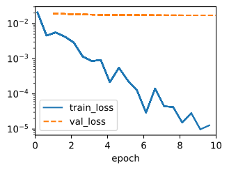
L2 norm of w: 0.011104541830718517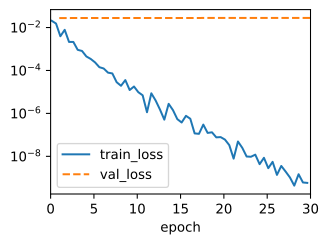
L2 norm of w: 0.010900448076426983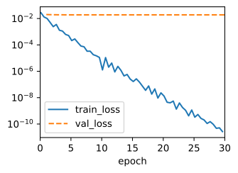
L2 norm of w: 0.011438996531069279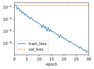
2.7.3.4 Using Weight Decay
Below, we run with substantial weight decay. Note that the training error increases but the validation error decreases. This is precisely the effect we expect from regularization.
train_scratch(3)L2 norm of w: 0.000481135182781145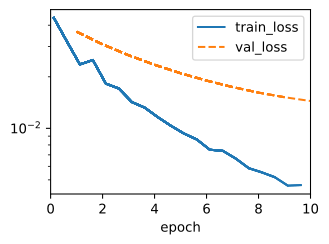
L2 norm of w: 0.0003025034093298018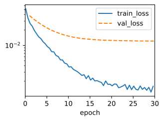
L2 norm of w: 0.0007521652150899172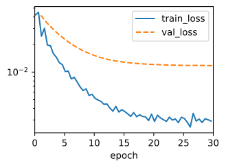
L2 norm of w: 0.0010663290740922093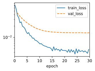
2.7.3.5 Why Shrinkage Helps: The Spectral View
The geometry of Figure 2.7.1 says that the penalty pulls \(\hat{\mathbf{w}}\) toward the origin, but not which parts of \(\hat{\mathbf{w}}\) are pulled hardest. For linear regression we can say exactly. Adding the penalty keeps the problem quadratic, so it retains a closed-form solution (dropping the unpenalized intercept, which centering absorbs). Minimizing
\[\frac{1}{2}\|\mathbf{y} - \mathbf{X}\mathbf{w}\|^2 + \frac{\tilde{\lambda}}{2}\|\mathbf{w}\|^2 \tag{2.7.8}\]
gives the ridge estimator
\[\mathbf{w}^*_{\tilde{\lambda}} = (\mathbf{X}^\top \mathbf{X} + \tilde{\lambda} \mathbf{I})^{-1} \mathbf{X}^\top \mathbf{y}, \tag{2.7.9}\]
which is well defined for every \(\tilde{\lambda} > 0\) even when \(\mathbf{X}^\top \mathbf{X}\) is singular; this is the estimator promised in the last part of exercise 3 of Section 2.1. (Because the loss \(L\) of this section averages over the \(n\) examples while the objective above sums, the two conventions are related by \(\tilde{\lambda} = n\lambda\).)
To see what this estimator does, substitute the singular value decomposition \(\mathbf{X} = \mathbf{U}\mathbf{D}\mathbf{V}^\top\) (Section 24.3). A short calculation shows that the ridge prediction is
\[\mathbf{X}\mathbf{w}^*_{\tilde{\lambda}} = \sum_j \mathbf{u}_j\, \frac{d_j^2}{d_j^2 + \tilde{\lambda}}\, \mathbf{u}_j^\top \mathbf{y}, \tag{2.7.10}\]
whereas ordinary least squares gives \(\sum_j \mathbf{u}_j \mathbf{u}_j^\top \mathbf{y}\), the orthogonal projection from Section 2.1. Ridge therefore shrinks the response along the \(j\)-th principal direction of the data by the factor \(d_j^2 / (d_j^2 + \tilde{\lambda})\). Directions with large singular value \(d_j\) (strongly represented in the data) pass through almost untouched, while directions with small \(d_j\), where a little noise in \(\mathbf{y}\) produces a wild swing in \(\mathbf{w}\), are suppressed hardest. This is the quantitative reason shrinkage tames overfitting: it damps precisely the directions that the data constrains least, the ones a noise-chasing fit exploits. Summing the per-direction factors yields the effective degrees of freedom
\[\textrm{df}(\tilde{\lambda}) = \sum_j \frac{d_j^2}{d_j^2 + \tilde{\lambda}}, \tag{2.7.11}\]
which slides continuously from \(\textrm{rank}(\mathbf{X})\) at \(\tilde{\lambda} = 0\) toward \(0\) as \(\tilde{\lambda} \to \infty\), the “continuous complexity dial” from the start of this section, made literal. We compute these quantities on the dataset used above.
d = torch.linalg.svdvals(data.X[:data.num_train])
for lam in (0, 3, 30):
    shrink = d**2 / (d**2 + data.num_train * lam)
    print(f'lambda={lam:2d}  df={float(d2l.reduce_sum(shrink)):5.1f}  '
          f'strongest {float(shrink[0]):.2f}  weakest {float(shrink[-1]):.2f}')
lambda= 0 df= 20.0 strongest 1.00 weakest 1.00
lambda= 3 df= 15.1 strongest 0.84 weakest 0.65
lambda=30 df= 4.9 strongest 0.34 weakest 0.16d = tf.linalg.svd(data.X[:data.num_train], compute_uv=False)
for lam in (0, 3, 30):
shrink = d**2 / (d**2 + data.num_train * lam)
print(f'lambda={lam:2d} df={float(d2l.reduce_sum(shrink)):5.1f} '
f'strongest {float(shrink[0]):.2f} weakest {float(shrink[-1]):.2f}')lambda= 0 df= 20.0 strongest 1.00 weakest 1.00
lambda= 3 df= 15.2 strongest 0.85 weakest 0.65
lambda=30 df= 5.0 strongest 0.36 weakest 0.16d = jnp.linalg.svd(data.X[:data.num_train], compute_uv=False)
for lam in (0, 3, 30):
shrink = d**2 / (d**2 + data.num_train * lam)
print(f'lambda={lam:2d} df={float(d2l.reduce_sum(shrink)):5.1f} '
f'strongest {float(shrink[0]):.2f} weakest {float(shrink[-1]):.2f}')lambda= 0 df= 20.0 strongest 1.00 weakest 1.00
lambda= 3 df= 15.2 strongest 0.84 weakest 0.63
lambda=30 df= 5.0 strongest 0.35 weakest 0.15_, d, _ = np.linalg.svd(data.X[:data.num_train])
for lam in (0, 3, 30):
shrink = d**2 / (d**2 + data.num_train * lam)
print(f'lambda={lam:2d} df={float(d2l.reduce_sum(shrink)):5.1f} '
f'strongest {float(shrink[0]):.2f} weakest {float(shrink[-1]):.2f}')lambda= 0 df= 20.0 strongest 1.00 weakest 1.00
lambda= 3 df= 15.2 strongest 0.84 weakest 0.63
lambda=30 df= 4.9 strongest 0.34 weakest 0.15Two things stand out. First, 20 training examples constrain at most 20 directions of the 200-dimensional weight space: \(\textrm{rank}(\mathbf{X}) = 20\), so \(\textrm{df}(0) = 20\). Every gradient lies in the row space of \(\mathbf{X}\), so gradient descent never changes the component of \(\mathbf{w}\) in the 180-dimensional nullspace. Exercise 5 examines what this implies for the random initialization that WeightDecayScratch uses. Second, at the \(\lambda = 3\) that lowered the validation loss above, every shrinkage factor drops below one, the weakest directions are damped most, and \(\textrm{df}(\lambda)\) falls well below 20: the regularized model behaves like one with far fewer parameters than its nominal 200, which is exactly the continuous capacity control weight decay provides (Section 2.6).
2.7.4 Concise Implementation
Because weight decay is ubiquitous in neural network optimization, deep learning frameworks make it especially convenient, integrating weight decay into the optimization algorithm itself for easy use in combination with any loss function. Moreover, this integration serves a computational benefit, allowing implementation tricks to add weight decay to the algorithm, without any additional computational overhead. The weight decay portion of the update depends only on the current value of each parameter, and the optimizer must touch each parameter once anyway.
Below, we specify the weight decay hyperparameter directly through weight_decay when instantiating our optimizer. By default, PyTorch decays both weights and biases simultaneously, but we can configure the optimizer to handle different parameters according to different policies. Here, we only set weight_decay for the weights (the net.weight parameters), hence the bias (the net.bias parameter) will not decay.
Below, we create an \(\ell_2\) regularizer with the weight decay hyperparameter wd and apply it to the layer’s weights through the kernel_regularizer argument.
Below, we specify the weight decay hyperparameter directly through wd when instantiating our Trainer. By default, Gluon decays both weights and biases simultaneously. Note that the hyperparameter wd will be multiplied by wd_mult when updating model parameters. Thus, if we set wd_mult to zero, the bias parameter \(b\) will not decay.
class WeightDecay(d2l.LinearRegression):
    def __init__(self, wd, lr):
        super().__init__(lr)
        self.save_hyperparameters()
        self.wd = wd

    def configure_optimizers(self):
        return torch.optim.SGD([
            {'params': self.net.weight, 'weight_decay': self.wd},
            {'params': self.net.bias}], lr=self.lr)
class WeightDecay(d2l.LinearRegression):
def __init__(self, wd, lr):
super().__init__(lr)
self.save_hyperparameters()
# Keras' l2(wd) penalty is wd*sum(w**2) (no 1/2 factor), so use
# wd/2 to match the (wd/2)*||w||^2 convention used elsewhere.
self.net = tf.keras.layers.Dense(
1, kernel_regularizer=tf.keras.regularizers.l2(wd / 2),
kernel_initializer=tf.keras.initializers.RandomNormal(0, 0.01)
)
def loss(self, y_hat, y):
return super().loss(y_hat, y) + tf.add_n(self.net.losses)class WeightDecay(d2l.LinearRegression):
def __init__(self, wd, lr, num_inputs=200, rngs=None):
super().__init__(num_inputs, lr, rngs=rngs)
self.save_hyperparameters(ignore=['rngs'])
def configure_optimizers(self):
# Weight Decay is not available directly within optax.sgd, but
# optax allows chaining several transformations together. We
# mask the decay so it applies to the kernel only (not bias),
# matching the per-parameter-group convention in PyTorch / MXNet.
def kernel_mask(params):
return jax.tree_util.tree_map_with_path(
lambda path, _: getattr(path[-1], 'name', None) == 'kernel',
params)
return optax.chain(
optax.masked(optax.add_decayed_weights(self.wd), kernel_mask),
optax.sgd(self.lr))class WeightDecay(d2l.LinearRegression):
def __init__(self, wd, lr):
super().__init__(lr)
self.save_hyperparameters()
self.wd = wd
def configure_optimizers(self):
for p in self.collect_params('.*bias').values():
p.wd_mult = 0
return gluon.Trainer(self.collect_params(),
'sgd',
{'learning_rate': self.lr, 'wd': self.wd})This version runs faster and is easier to implement than the from-scratch code, benefits that grow more pronounced on larger problems and as this work becomes routine. One subtlety: a framework’s weight_decay adds the term \(\lambda\mathbf{w}\) to the gradient, whereas our from-scratch penalty added \(\frac{\lambda}{2}\|\mathbf{w}\|^2\) to the loss. When the loss omits the \(\frac{1}{2}\) factor (as PyTorch’s nn.MSELoss does), the two correspond to slightly different effective values of \(\lambda\), so the converged \(\|\mathbf{w}\|^2\) need not match the from-scratch value exactly, even though the regularizing effect is the same.
model = WeightDecay(wd=3, lr=0.01)
model.board.yscale='log'
trainer.fit(model, data)

print('L2 norm of w:', float(l2_penalty(model.get_w_b()[0]).detach()))
L2 norm of w: 0.0006812948267906904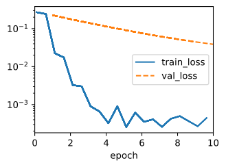
model = WeightDecay(wd=3, lr=0.01)
model.board.yscale='log'
trainer.fit(model, data)

print('L2 norm of w:', float(l2_penalty(model.get_w_b()[0])))
L2 norm of w: 0.00038615940138697624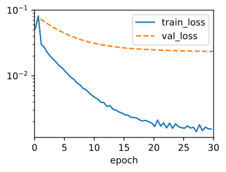
model = WeightDecay(wd=3, lr=0.01)
model.board.yscale='log'
trainer.fit(model, data)

print('L2 norm of w:', float(l2_penalty(model.get_w_b()[0])))
L2 norm of w: 0.011407211422920227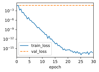
model = WeightDecay(wd=3, lr=0.01)
model.board.yscale='log'
trainer.fit(model, data)

print('L2 norm of w:', float(l2_penalty(model.get_w_b()[0])))
L2 norm of w: 0.0012607135577127337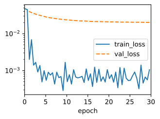
So far we have measured complexity through the norm of a linear function’s weights. The same principle extends to the nonlinear functions a deep network computes: in practice, weight decay is often applied to each layer’s weights. We use this convention throughout the book while treating choices such as bias decay separately.
2.7.5 Summary
Weight decay adds an \(\ell_2\) penalty to the training objective. Geometrically, the penalty expresses a preference for smaller weight norms; under SGD, it appears as multiplicative shrinkage in each update. In linear regression, the spectral view shows that ridge suppresses directions that the data constrain weakly, continuously reducing the effective degrees of freedom.
With Gaussian observation noise and a zero-mean Gaussian prior on the weights, the same objective is MAP estimation, with \(\lambda=\sigma^2/(n\tau^2)\) for the averaged-loss convention used here. Framework optimizers implement weight decay directly and allow parameter groups to follow different update rules. The value of \(\lambda\) is selected on validation data, not from training error alone.
2.7.6 Exercises
[code] The \(\lambda\) sweep. Train
WeightDecayScratchonDatafor \(\lambda \in \{0, 0.1, 0.3, 1, 3, 10, 30\}\). The loss thatWeightDecayScratchreports includes the penalty, so measure the final training and validation losses with the unpenalized squared loss ofd2l.LinearRegressionScratch.- Plot both losses against the nonzero values of \(\lambda\) on a logarithmic \(\lambda\) axis, draw the \(\lambda = 0\) losses as horizontal reference lines, and report the \(\lambda^*\) with the smallest validation loss.
- Compute \(\textrm{df}(\lambda)\) for the same values with the code of Section 2.7.3.5 and re-plot the validation loss against \(\textrm{df}(\lambda)\). Compare the shape with Figure 2.6.1.
- Repeat the search of (a) on two more random train/validation splits of the same data (permute the rows of
data.Xanddata.ywith the same permutation). Report whether \(\lambda^*\) is stable across the three splits and by how much the validation loss differs between \(\lambda^*\) and its runner-up.
The \(\ell_1\) update. Replace the penalty \(\frac{\lambda}{2}\|\mathbf{w}\|^2\) by \(\lambda \sum_i |w_i|\) (\(\ell_1\) regularization).
- Derive the minibatch SGD update for \(\mathbf{w}\), using the subgradient \(\operatorname{sign}(w_i)\) of Section 2.1 in place of the derivative of \(|w_i|\).
- Compare the change that the penalty alone makes to \(w_i\) in one step of this update with the change it makes in the \(\ell_2\) update of this section, once for large and once for small \(|w_i|\).
- The update of (a) almost never sets \(w_i\) exactly to zero. Split it into a gradient step on \(L\) followed by the penalty step, and modify the penalty step so that it sets \(w_i\) to zero whenever it would change the sign of \(w_i\). Relate the result to the feature selection that lasso performs.
Frobenius penalty. Weight decay on a layer with weight matrix \(\mathbf{W} \in \mathbb{R}^{q \times d}\) adds \(\frac{\lambda}{2}\|\mathbf{W}\|_\textrm{F}^2\) to the loss, with the Frobenius norm of Section 1.3.4.
- The trace \(\textrm{tr}(\mathbf{A})\) of a square matrix \(\mathbf{A}\) is the sum of its diagonal entries. Show that \(\|\mathbf{W}\|_\textrm{F}^2 = \textrm{tr}(\mathbf{W}^\top \mathbf{W})\), the matrix analogue of \(\|\mathbf{w}\|^2 = \mathbf{w}^\top \mathbf{w}\).
- Show that \(\|\mathbf{W}\mathbf{v}\| \le \|\mathbf{W}\|_\textrm{F}\,\|\mathbf{v}\|\) for every \(\mathbf{v} \in \mathbb{R}^d\). Use it to bound the change of the output \(\mathbf{W}\mathbf{x}\) when the input \(\mathbf{x}\) is perturbed by \(\boldsymbol{\delta}\).
[code] Early stopping. Train
WeightDecayScratchwith \(\lambda = 0\) as intrain_scratch(0)for at most 30 epochs. Record the validation loss after every epoch, and stop when it has not improved for three consecutive epochs. Report the epoch with the lowest validation loss and that loss. Compare it with the final validation losses oftrain_scratch(0)andtrain_scratch(3), measuring the validation loss oftrain_scratch(3)without its penalty term.Decay of the nullspace. ● Let \(\mathbf{X}\) be the \(20 \times 200\) matrix of training inputs.
- Show that one minibatch SGD step of
WeightDecayScratchmultiplies the component of \(\mathbf{w}\) in the nullspace of \(\mathbf{X}\) by \(1 - \eta\lambda\). WeightDecayScratchdraws its initial weights from \(\mathcal{N}(0, 0.01^2)\). Estimate how much the nullspace component of the initial weights adds to the validation loss, and use the estimate with (a) to explain the comparison of the early-stopped run withtrain_scratch(3)in exercise 4.
- Show that one minibatch SGD step of
[code] Ridge as augmented least squares. Center the columns of
data.Xand the labelsdata.yof the training split so that the intercept drops out, and implement ridge regression two ways.- Use the closed form \((\mathbf{X}^\top\mathbf{X}+\tilde{\lambda}\mathbf{I})^{-1}\mathbf{X}^\top\mathbf{y}\) of Section 2.7.3.5.
- Run ordinary least squares on \(\mathbf{X}\) stacked with \(\sqrt{\tilde{\lambda}}\,\mathbf{I}\) and \(\mathbf{y}\) stacked with \(d\) zeros.
Confirm that the two give matching \(\hat{\mathbf{w}}\) up to numerical precision. With \(\tilde{\lambda} = n\lambda = 60\), compare
l2_penaltyof your solution with the value printed bytrain_scratch(3).Adapted from Hastie, Tibshirani, and Friedman, The Elements of Statistical Learning, Exercise 3.12.
MAP estimation. The derivation in this section gives \(\lambda = \sigma^2/(n\tau^2)\) for the prior \(\mathbf{w} \sim \mathcal{N}(\mathbf{0}, \tau^2\mathbf{I})\) and noise variance \(\sigma^2\).
- For
train_scratch(3)(\(n = 20\), \(\sigma = 0.01\), \(\lambda = 3\)), compute \(\tau\) and compare it with the true weights \(w_i = 0.01\) ofData. Is the implied prior consistent with the data-generating process? Then compute the \(\lambda\) that a prior with \(\tau = 0.01\) implies. - Holding \(\tau\) and \(\sigma\) fixed, describe how \(\lambda\) changes as \(n\) grows and interpret the change in terms of the relative weight of prior and likelihood.
- The bias \(b\) is not penalized. Which prior on \(b\) does this correspond to?
- For
Shrinkage versus penalty. Weight decay can be applied by shrinking the weights before the gradient step or by adding \(\frac{\lambda}{2}\|\mathbf{w}\|^2\) to the loss \(L\).
Show that the weight-decay update \(\mathbf{w} \leftarrow (1-\eta\lambda)\mathbf{w} - \eta\nabla L\) of this section is identical to a gradient step on the penalized loss \(L + \frac{\lambda}{2}\|\mathbf{w}\|^2\).
Suppose that the gradient of \(L\) is rescaled coordinate-wise by fixed constants \(a_i > 0\) before the step. Shrinking and then stepping gives the first update below, and stepping on the penalized gradient gives the second:
\[w_i \leftarrow (1-\eta\lambda)\, w_i - \eta a_i \,\partial_{w_i} L \qquad \textrm{and} \qquad w_i \leftarrow w_i - \eta a_i \left(\partial_{w_i} L + \lambda w_i\right). \tag{2.7.12}\]
Determine for which \(a_i\) the two coincide and the factor by which the second update shrinks coordinate \(i\). Relate your finding to the decoupled weight decay of AdamW (Section 9.7).
Adapted from Simon Prince, Understanding Deep Learning, Problem 9.5.