theta, n = 1.5, 200_000
z = np.random.default_rng().standard_normal(n)     # noise, independent of theta
x = theta + z                                      # samples of N(theta, 1)
pathwise = 2 * x                                   # d/dtheta (theta + z_i)^2
score = x**2 * z                                   # g(x) times the score x - theta
baseline = (x**2 - (theta**2 + 3)) * z             # with the optimal baseline
exact_sd = {'pathwise': 2, 'score': math.sqrt(theta**4 + 14 * theta**2 + 15),
            'score+baseline': math.sqrt(8 * theta**2 + 6)}
print(f'true derivative 2*theta = {2 * theta}')
for name, s in zip(exact_sd, [pathwise, score, baseline]):
    print(f'{name:15s} mean={s.mean():.4f}  sd={s.std():.3f} '
f'(exact {exact_sd[name]:.3f}) se={s.std() / math.sqrt(n):.4f}')34.7 Expectations and Their Gradients
Every loss we have minimized was an average: over a minibatch, over the masks of dropout, over the noise added to an input. As long as the randomness does not depend on the parameters, such an average is easy to differentiate. The derivative of an average is the average of the derivatives, and minibatch gradient descent computes it without a second thought. The difficulty begins when the parameters control the distribution itself. A variational autoencoder draws its latent code from a distribution that its encoder outputs. A policy-gradient method (Section 14.6) draws actions from the very policy it is trying to improve. The loss is then an expectation over samples whose distribution moves with the parameters, and a sample, once drawn, is just a number: it does not remember the parameter that produced it.
Here is the smallest such problem. Let \(X\sim\mathcal N(\theta,1)\), a normal variable with mean \(\theta\), and let the loss be
\[ \ell(\theta)=\mathbb{E}\bigl[X^2\bigr]=\theta^2+1 . \]
The value follows by writing \(X=\theta+Z\) with \(Z\) standard normal: \(\mathbb{E}[(\theta+Z)^2]=\theta^2+2\theta\,\mathbb{E}[Z]+\mathbb{E}[Z^2]\), where \(\mathbb{E}[Z]=0\) by symmetry and \(\mathbb{E}[Z^2]=1\) (Section 34.6.2.3). At \(\theta=1.5\) the derivative is \(\ell'(1.5)=3\). A real model can draw samples of \(X\), but it cannot write \(\ell\) in closed form. How do we estimate \(\ell'(\theta)\) from samples?
Calculus gives two answers, and they differ in kind. Both write the expectation as an integral (Section 34.6) and move the derivative inside it. The score-function estimator then differentiates the density and leaves the samples alone. The pathwise estimator differentiates the samples and leaves the density alone. Neither always wins, and comparing the two (Section 34.7.3) is the main business of this section. Before that we recall what an expectation is, and settle when a derivative may be moved inside an integral, which is the step that needs care.
34.7.1 Expectations as Integrals
Before anything is differentiated we fix what an expectation is. The probability chapter treats the two definitions below at length (Section 36.1); here they are a recall, in the language of the previous section. A probability density on a set \(\mathcal X\) is a nonnegative function whose total integral is \(1\):
\[ p(x)\ge 0, \qquad \int_{\mathcal X} p(x)\,dx = 1 . \tag{34.7.1}\]
A random variable \(X\) with density \(p\) falls in an interval with probability equal to the area above it, \(P(a\le X\le b)=\int_a^bp(x)\,dx\) (Equation 36.1.3). Being a probability per unit length and not a probability, a density can exceed \(1\): the uniform density on \([0,\tfrac12]\) equals \(2\). Our standard example is the standard normal \(\mathcal N(0,1)\) with density \(p(z)=e^{-z^2/2}/\sqrt{2\pi}\), whose constant is the Gaussian integral of Section 34.6.
An expectation averages a function of \(X\), weighting each value by its density:
\[ \mathbb{E}[X] = \int_{\mathcal X} x\,p(x)\,dx, \qquad \mathbb{E}[g(X)] = \int_{\mathcal X} g(x)\,p(x)\,dx . \tag{34.7.2}\]
The expectation \(\mathbb{E}[g(X)]\) is defined when \(\int_{\mathcal X}|g(x)|\,p(x)\,dx<\infty\); the Cauchy density of exercise 3 has no mean for this reason.
Most expectations in deep learning have no closed form, and many are over thousands of dimensions, where no grid is affordable. They are estimated by drawing samples \(x_1,\ldots,x_n\) from \(p\) and averaging, \(\frac1n\sum_ig(x_i)\). This is the Monte Carlo estimate. If one sample \(g(X)\) has standard deviation \(\sigma\), the estimate has root-mean-square error \(\sigma/\sqrt n\), whatever the dimension (Section 36.5.1.7). The gradient estimators of this section are Monte Carlo estimates of this kind. Two unbiased estimators of the same gradient differ only in the spread of a single sample, so its standard deviation \(\sigma\) is what we compare.
34.7.2 Differentiation under the Integral Sign
34.7.2.1 The Swap
The loss \(\ell(\theta)=\mathbb{E}[X^2]\) is an integral that depends on a parameter. A parameter can enter an integral in two places: through the limits of integration, which the fundamental theorem Equation 34.6.3 handles, or through the integrand.
For the integrand, the derivative passes inside the integral:
\[ \frac{d}{d\theta} \int f(x, \theta)\,dx = \int \frac{\partial f}{\partial\theta}(x, \theta)\,dx . \tag{34.7.3}\]
The rate of change of the area is the integral of the rate of change of the height. We call this exchange of derivative and integral the swap, and both gradient estimators rest on it. It looks innocent, since a derivative is a limit of difference quotients and an integral a limit of sums, and finite sums and differences commute. But two limits are being exchanged, and that needs a hypothesis. On a bounded range of \(x\) it holds when \(\partial_\theta f\) is continuous in both variables. On an infinite range it needs in addition an integrable function of \(x\) that bounds \(|\partial_\theta f(x,\theta')|\) for all \(\theta'\) near \(\theta\) (a consequence of dominated convergence, quoted without proof from (Folland 1999)). For \(f(x,\theta)=x^2p_\theta(x)\) with the normal density such a bound exists, because the Gaussian factor dominates every polynomial.
34.7.2.2 The Leibniz Rule
The swap alone is wrong when the limits of integration move with the parameter. The Leibniz rule supplies the correction: the two effects add (Figure 34.7.1).
Proposition (Leibniz rule). Let \(f\) and \(\partial_\theta f\) be continuous on a region containing \(\{(x,\theta):x\in[a(\theta),b(\theta)]\}\) for \(\theta\) in an open interval, and let \(a\) and \(b\) be differentiable. Then
\[ \frac{d}{d\theta} \int_{a(\theta)}^{b(\theta)} f(x, \theta)\,dx = \int_{a(\theta)}^{b(\theta)} \frac{\partial f}{\partial\theta}(x,\theta)\,dx + f\bigl(b(\theta), \theta\bigr)\,b'(\theta) - f\bigl(a(\theta), \theta\bigr)\,a'(\theta) . \tag{34.7.4}\]
Proof. Let \(H(\alpha,\beta,\theta)=\int_\alpha^\beta f(x,\theta)\,dx\). By the fundamental theorem, \(\partial_\beta H=f(\beta,\theta)\) and \(\partial_\alpha H=-f(\alpha,\theta)\). By the swap on the bounded range \([\alpha,\beta]\), \(\partial_\theta H=\int_\alpha^\beta\partial_\theta f\,dx\). All three partial derivatives are continuous, so the chain rule of Section 34.3 applies to \(\theta\mapsto H(a(\theta),b(\theta),\theta)\) and adds the three contributions, weighted by \(a'(\theta)\), \(b'(\theta)\) and \(1\). \(\blacksquare\)
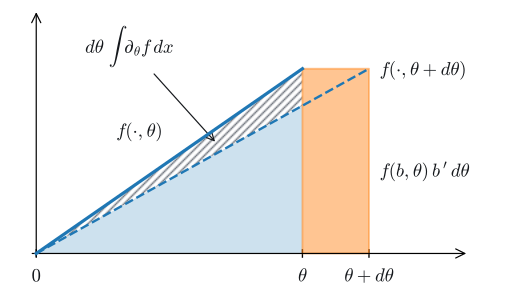
Dropping the boundary term gives a wrong answer. Let \(X\) be uniform on \([0,\theta]\), with density \(1/\theta\) there. Then \(\mathbb{E}[X]=\int_0^\theta\frac x\theta\,dx=\frac\theta2\), with derivative \(+\tfrac12\). Differentiating only the integrand gives \(\int_0^\theta-\frac{x}{\theta^2}\,dx=-\tfrac12\), the wrong sign. The boundary term \(f(\theta,\theta)\,b'(\theta)=\frac\theta\theta\cdot1=1\) restores \(-\tfrac12+1=+\tfrac12\). Whenever the support of a density moves with the parameter, the plain swap is not enough (exercise 1 does \(\mathbb{E}[X^2]\)).
34.7.2.3 Log-Integral-Exp
The swap also gives the continuous version of this chapter’s log-sum-exp. Differentiating \(\log\int e^{\theta x}p(x)\,dx\) with the chain rule and Equation 34.7.3 gives
\[ \frac{d}{d\theta}\log\int e^{\theta x}p(x)\,dx=\frac{\int x\,e^{\theta x}p(x)\,dx}{\int e^{\theta x}p(x)\,dx}, \]
the mean of \(x\) under the tilted density \(e^{\theta x}p(x)/\int e^{\theta x}p\). For the standard normal, completing the square, \(\theta z-\tfrac12z^2=\tfrac12\theta^2-\tfrac12(z-\theta)^2\), shows that the tilted density is \(\mathcal N(\theta,1)\) and that \(\log\mathbb{E}[e^{\theta Z}]=\theta^2/2\), whose derivative \(\theta\) is indeed the tilted mean. The gradient of log-sum-exp is the softmax; the gradient of log-integral-exp is an expectation. This is the derivative \(A'(\eta)\) of the log-partition function in Section 36.4.
34.7.3 Score-Function and Pathwise Gradients
By the swap, the derivative of an expectation is an integral, \(\int g(x)\,\partial_\theta p_\theta(x)\,dx\). Unfortunately it is not an expectation: \(\partial_\theta p_\theta\) is not a density, and we cannot draw samples from it. Two identities turn the integral into an expectation that samples can estimate.
34.7.3.1 The Score-Function Estimator
Write \(p_{\boldsymbol\theta}\) for a density that depends on parameters \(\boldsymbol\theta\). The chain rule for \(\log\) gives the log-derivative identity
\[ \nabla_{\boldsymbol\theta}\,p_{\boldsymbol\theta}(x)=p_{\boldsymbol\theta}(x)\,\nabla_{\boldsymbol\theta}\log p_{\boldsymbol\theta}(x). \tag{34.7.5}\]
The gradient of a density is the density times the gradient of its logarithm, the score \(\nabla_{\boldsymbol\theta}\log p_{\boldsymbol\theta}\). When the swap is valid and the support of \(p_{\boldsymbol\theta}\) does not move with \(\boldsymbol\theta\), the score has mean zero: \(\mathbb{E}[\nabla_{\boldsymbol\theta}\log p_{\boldsymbol\theta}(X)]=\int\nabla_{\boldsymbol\theta}p_{\boldsymbol\theta}\,dx=\nabla_{\boldsymbol\theta}\int p_{\boldsymbol\theta}\,dx=\nabla_{\boldsymbol\theta}1=\mathbf 0\). The uniform density on \([0,\theta]\) shows why the support matters: its score is \(\partial_\theta\log(1/\theta)=-1/\theta\), whose mean is \(-1/\theta\ne0\), because differentiating \(\int_0^\theta p_\theta=1\) also produces the boundary term \(p_\theta(\theta)=1/\theta\). The mean-zero score is the starting point of Fisher information (Section 36.6).
Multiplying the identity by \(g\) and integrating gives the score-function identity, for \(g\) that does not depend on \(\boldsymbol\theta\):
\[ \nabla_{\boldsymbol{\theta}}\,\mathbb{E}_{X\sim p_{\boldsymbol{\theta}}}[g(X)] =\int g(x)\,\nabla_{\boldsymbol\theta}p_{\boldsymbol\theta}(x)\,dx = \mathbb{E}\bigl[g(X)\,\nabla_{\boldsymbol{\theta}}\log p_{\boldsymbol{\theta}}(X)\bigr]. \tag{34.7.6}\]
The gradient of an expected loss is the average loss, weighted by how much the parameter raises the log-probability of each sample. It is estimated by Monte Carlo: sample \(x_i\), average \(g(x_i)\nabla\log p_{\boldsymbol\theta}(x_i)\). This is the REINFORCE estimator of policy-gradient methods (Williams 1992). If \(g\) also depends on \(\boldsymbol\theta\), add \(\mathbb{E}[\nabla_{\boldsymbol\theta}g(X,\boldsymbol\theta)]\).
Because the score has mean zero, any baseline \(b\) that does not depend on \(x\) can be subtracted from \(g\) without changing the mean: \(\mathbb{E}[(g(X)-b)\nabla\log p_{\boldsymbol\theta}(X)]=\mathbb{E}[g(X)\nabla\log p_{\boldsymbol\theta}(X)]\). A good \(b\) lowers the variance.
34.7.3.2 The Pathwise Estimator
The second identity gives the sample its memory back. Often a sample can be produced by transforming noise that does not depend on \(\boldsymbol\theta\): \(x=T_{\boldsymbol\theta}(\mathbf z)\) with \(\mathbf z\sim q\). The normal \(\mathcal N(\mu,\sigma^2)\) is \(\mu+\sigma z\) with \(z\sim\mathcal N(0,1)\). Then the expectation is an integral over \(\mathbf z\), whose density \(q\) does not move, and the swap gives the pathwise identity
\[ \nabla_{\boldsymbol\theta}\, \mathbb{E}_{X\sim p_{\boldsymbol\theta}}[g(X)] =\nabla_{\boldsymbol\theta}\int g\bigl(T_{\boldsymbol\theta}(\mathbf z)\bigr)\,q(\mathbf z)\,d\mathbf z =\mathbb{E}_{\mathbf z\sim q} \Bigl[\nabla_{\boldsymbol\theta}\, g\bigl(T_{\boldsymbol\theta}(\mathbf z)\bigr)\Bigr]. \tag{34.7.7}\]
The estimator differentiates the sample itself: automatic differentiation follows the path from \(\boldsymbol\theta\) through \(T_{\boldsymbol\theta}\) to \(g\). This reparameterization is how variational autoencoders backpropagate through a Gaussian latent variable (Kingma and Welling 2014). It needs \(T\) differentiable in \(\boldsymbol\theta\), \(g\) differentiable along the path (a Lipschitz \(g\) suffices when \(X\) has a density), and a dominating bound for the swap. No boundary term appears, even when the support of \(X\) moves, because the integral is over \(\mathbf z\) and \(q\) stays put.
The hypothesis on \(g\) cannot be dropped. Take \(g(x)=\mathbf{1}(x>0)\), which is \(1\) for positive \(x\) and \(0\) otherwise, and \(X=\theta+z\). Then \(\mathbb{E}[g(X)]=P(z>-\theta)\) has derivative \(\varphi(\theta)=e^{-\theta^2/2}/\sqrt{2\pi}\), which is \(0.13\) at \(\theta=1.5\). The pathwise sample \(\partial_\theta\mathbf{1}(\theta+z>0)\) is \(0\) for every \(z\) except \(z=-\theta\), an event of probability zero, so the pathwise estimator returns \(0\). The score sample \(\mathbf{1}(x>0)\,z\) has mean \(\int_{-\theta}^\infty z\,\varphi(z)\,dz=\bigl[-\varphi(z)\bigr]_{-\theta}^\infty=\varphi(\theta)\), the right answer. The score estimator never differentiates through the sample, which is why it also covers Bernoulli and categorical choices, where no differentiable path from \(\boldsymbol\theta\) to the sample exists.
34.7.3.3 The Two Estimators Compared
We now have two unbiased estimators of the same derivative, and the smallest problem is simple enough to compute the variance of both by hand. For \(\ell(\theta)=\mathbb{E}[X^2]\) with \(X=\theta+z\), one sample contributes \(2X\) to the pathwise estimator, with variance \(\textrm{Var}(2X)=4\). The score of the normal location family is \(\partial_\theta\log p_\theta(X)=X-\theta=z\), so one sample contributes \(X^2z\) to the score-function estimator, and \((X^2-b)z\) with a baseline. The variance of \(X^2z\) needs the Gaussian moments \(\mathbb{E}[z^2]=1\), \(\mathbb{E}[z^4]=3\) and \(\mathbb{E}[z^6]=15\), all from Stein’s identity \(\mathbb{E}[g'(Z)]=\mathbb{E}[Z\,g(Z)]\) (Section 34.6.2.3). The odd powers of \(z\) drop out of the second moment,
\[ \mathbb{E}\bigl[(\theta+z)^4z^2\bigr]=\theta^4\,\mathbb{E}[z^2]+6\theta^2\,\mathbb{E}[z^4]+\mathbb{E}[z^6]=\theta^4+18\theta^2+15, \]
and subtracting the squared mean \((2\theta)^2\) leaves the variance \(\theta^4+14\theta^2+15\). The variance-minimizing constant baseline is \(b^\star=\theta^2+3\), and it leaves \(8\theta^2+6\) (exercise 2). At \(\theta=1.5\) the three standard deviations are \(2\) for the pathwise estimator, \(7.18\) for the score function, and \(4.90\) with the baseline. The baseline helps, but it cannot close the gap for this \(g\), since \(8\theta^2+6>4\) for every \(\theta\).
A simulation can test all of this at once. The pathwise sample is \(\partial_\theta(\theta+z_i)^2=2x_i\), so no automatic differentiation is needed. If the closed forms are right, the three sample standard deviations should come out near \(2\), \(7.18\) and \(4.90\), and each mean should lie within a few standard errors \(\mathrm{sd}/\sqrt n\) of \(3\).
true derivative 2*theta = 3.0
pathwise        mean=3.0041  sd=2.000 (exact 2.000)  se=0.0045
score           mean=3.0068  sd=7.146 (exact 7.181)  se=0.0160
score+baseline  mean=2.9961  sd=4.858 (exact 4.899)  se=0.0109
true derivative 2*theta = 3.0
pathwise mean=3.0086 sd=1.997 (exact 2.000) se=0.0045
score mean=3.0114 sd=7.137 (exact 7.181) se=0.0160
score+baseline mean=2.9887 sd=4.852 (exact 4.899) se=0.0108true derivative 2*theta = 3.0
pathwise mean=3.0029 sd=2.001 (exact 2.000) se=0.0045
score mean=3.0204 sd=7.268 (exact 7.181) se=0.0163
score+baseline mean=3.0128 sd=4.960 (exact 4.899) se=0.0111true derivative 2*theta = 3.0
pathwise mean=3.0042 sd=2.002 (exact 2.000) se=0.0045
score mean=3.0228 sd=7.236 (exact 7.181) se=0.0162
score+baseline mean=3.0117 sd=4.940 (exact 4.899) se=0.0110In most runs the three means lie within about two standard errors of \(3\), and the sample standard deviations match the closed forms to within a few percent. With the same number of samples, the pathwise estimate is about \(3.6\) times more precise than the plain score estimate. Put differently, the score estimate needs about thirteen times as many samples for the same precision.
It would be wrong to conclude that the pathwise estimator always has the smaller variance. Take \(g(x)=\sin(\omega x)\), for which the derivative of the mean is \(\omega\cos(\omega\theta)e^{-\omega^2/2}\). The pathwise sample \(\omega\cos(\omega X)\) has standard deviation close to \(\omega/\sqrt2\), while the score sample \(\sin(\omega X)\,z\) has standard deviation at most \(\sqrt{\mathbb{E}[z^2]}=1\), because \(|\sin|\le1\). An oscillating integrand has large derivatives but bounded values. We compare the two at \(\omega=1\) and \(\omega=3\), reusing the samples.
for omega in [1, 3]:
    true = omega * math.cos(omega * theta) * math.exp(-omega**2 / 2)
    path, score = omega * np.cos(omega * x), np.sin(omega * x) * z
    print(f'omega={omega}  true={true:+.4f}  pathwise {path.mean():+.4f} '
f'(sd {path.std():.2f}) score {score.mean():+.4f} (sd {score.std():.2f})')omega=1 true=+0.0429 pathwise +0.0414 (sd 0.66) score +0.0432 (sd 0.54)
omega=3 true=-0.0070 pathwise -0.0067 (sd 2.12) score -0.0080 (sd 0.71)omega=1 true=+0.0429 pathwise +0.0403 (sd 0.66) score +0.0429 (sd 0.54)
omega=3 true=-0.0070 pathwise -0.0026 (sd 2.12) score -0.0083 (sd 0.70)omega=1 true=+0.0429 pathwise +0.0431 (sd 0.66) score +0.0405 (sd 0.55)
omega=3 true=-0.0070 pathwise -0.0025 (sd 2.12) score -0.0106 (sd 0.71)omega=1 true=+0.0429 pathwise +0.0420 (sd 0.66) score +0.0423 (sd 0.54)
omega=3 true=-0.0070 pathwise -0.0094 (sd 2.12) score -0.0054 (sd 0.71)At \(\omega=1\) the score estimator already has the smaller spread, about \(0.5\) against \(0.7\); at \(\omega=3\) it wins by a factor of three, about \(0.7\) against \(2.1\). Both means agree with the true values within a few standard errors.
Neither estimator wins everywhere, then. The pathwise estimator differentiates \(g\) and suffers where \(g'\) is large; the score-function estimator multiplies \(g\) by noise and suffers where \(g\) itself is large. In both, the standard deviation \(\sigma\) of a single sample decides how many samples are needed. It depends on the distribution the samples are drawn from, and choosing that distribution to make \(\sigma\) small, which is called importance sampling, is taken up in Section 36.8.
34.7.4 Summary
When a parameter moves the distribution of the samples, the gradient of an expected loss has to be rewritten as an expectation before samples can estimate it. Both ways of doing so move the derivative inside the integral, which needs a dominating bound and, when the limits move with the parameter, the boundary term of the Leibniz rule. The score-function identity differentiates the density. It works for any \(g\), including discrete choices, but its samples scale with \(g\) and can have high variance. The pathwise identity differentiates the sample. It needs a differentiable \(g\) and often, though not always, has the lower variance. Either estimate has root-mean-square error \(\sigma/\sqrt n\) (Section 36.5.1.7), so the standard deviation \(\sigma\) of one sample is the quantity to compare.
34.7.5 Exercises
- A moving support. Let \(X\) be uniform on \([0,\theta]\) with \(\theta>0\), so that \(\ell(\theta)=\mathbb{E}[X^2]=\int_0^\theta \tfrac{x^2}{\theta}\,dx=\tfrac{\theta^2}{3}\) and \(\ell'(\theta)=\tfrac{2\theta}{3}\).
- Differentiate \(\ell\) with the Leibniz rule Equation 34.7.4. Which part of the result does the plain swap Equation 34.7.3 produce, and which part does it miss?
- On the support, \(\log p_\theta(x)=-\log\theta\). Compute the expectation of the score-function estimator \(X^2\,\partial_\theta\log p_\theta(X)\) of Equation 34.7.6. Then let \(g\) be continuous on \([0,\infty)\). Show that the mean of \(g(X)\,\partial_\theta\log p_\theta(X)\) equals the plain swap Equation 34.7.3 applied to \(\mathbb{E}[g(X)]=\int_0^\theta g(x)\,p_\theta(x)\,dx\). What is its bias as an estimate of \(\frac{d}{d\theta}\mathbb{E}[g(X)]\), in terms of \(g(\theta)\) and \(\theta\)?
- Write \(X=\theta U\) with \(U\) uniform on \([0,1]\) and compute the expectation of the pathwise estimator of Equation 34.7.7. Why does it need no boundary term, although the support of \(X\) moves with \(\theta\)?
- [code] Estimator variance for a quartic. ● Let \(X\sim\mathcal N(\theta,1)\), write \(X=\theta+z\), and let \(s(X)=\partial_\theta\log p_\theta(X)=z\) be the score.
- Take \(g(X)=X^4\), so that \(\frac{d}{d\theta}\mathbb{E}[X^4]=4\theta^3+12\theta\). Derive the single-sample pathwise estimator from Equation 34.7.7 and the single-sample score-function estimator from Equation 34.7.6. Use the identity of exercise 7 (b) to show that both have mean \(4\theta^3+12\theta\).
- For a constant baseline \(b\), show that the variance of \((g(X)-b)\,s(X)\) is minimized by \(b^\star=\mathbb{E}[g(X)s(X)^2]/\mathbb{E}[s(X)^2]\). For \(g(X)=X^2\) show that \(b^\star=\theta^2+3\), and use \(\mathbb{E}[z^2]=1\), \(\mathbb{E}[z^4]=3\), \(\mathbb{E}[z^6]=15\) to derive the three variances \(4\), \(\theta^4+14\theta^2+15\) and \(8\theta^2+6\) that the text quotes.
- Evaluate \(b^\star\) for \(g(X)=X^4\). With \(10^6\) samples at \(\theta\in\{0,1,2\}\), estimate the standard deviations of the pathwise estimator, the score-function estimator, and the score-function estimator with the baseline. For which \(\theta\) is the baseline’s gain largest, and does it ever close the gap to the pathwise estimator? Explain the ordering from the sizes of \(g'\) and of \(g\).
- Take \(g(x)=\mathbf{1}(x>0)\) at \(\theta=1.5\). The text shows that the pathwise estimator is \(0\) for almost every sample, while the score-function estimator \(\mathbf{1}(x>0)\,z\) has the correct mean \(\varphi(\theta)=0.1295\). Verify both by simulation.
- [extended] Gradients through a coin flip. ●● When \(x\) is a discrete choice there is no differentiable path from \(\theta\) to the sample, so the pathwise estimator does not exist. Continuous relaxations such as Gumbel-softmax (Jang et al. 2017; Maddison et al. 2017) create a differentiable surrogate, and straight-through estimators (Bengio et al. 2013) use the hard sample in the forward pass and the surrogate in the backward pass; both are biased for the original objective. This problem measures that bias. Tucker et al. (2017) illustrate it on a toy problem. A single Bernoulli variable \(b\in\{0,1\}\) has \(P(b=1)=\sigma(\theta)\) for a logit \(\theta\), and the objective is \(\ell(\theta)=\mathbb{E}[(b-t)^2]\) with target \(t=0.45\). Let \(U\) be uniform on \((0,1)\), let \(\zeta=\log U-\log(1-U)\), and, for a temperature \(\tau>0\), let \(z=\sigma\bigl((\theta+\zeta)/\tau\bigr)\), the two-class case of the Gumbel-softmax relaxation.
- Compute \(\ell(\theta)\) and \(\ell'(\theta)\) in closed form. Which probability \(\sigma(\theta)\) minimizes \(\ell\), and does a finite \(\theta\) attain it?
- Show that \(b=\mathbf{1}(z>\tfrac12)\) satisfies \(P(b=1)=\sigma(\theta)\) for every \(\tau\).
- Implement three single-sample estimators of \(\ell'(\theta)\): REINFORCE Equation 34.7.6 with the baseline \(\ell(\theta)\); the relaxed estimator \(\frac{d}{d\theta}(z-t)^2\); and the straight-through estimator \(2(b-t)\frac{dz}{d\theta}\), which uses the hard sample in the loss and the relaxed sample in the derivative. Tabulate the mean and the standard deviation of each estimator against \(\ell'(\theta)\) for \(\theta\in\{-2,0,2\}\) and \(\tau\in\{1,0.5,0.1\}\). How does the bias of each estimator depend on \(\theta\) and \(\tau\)?
- Run stochastic gradient descent on \(\theta\) from \(\theta=0\) with step size \(1\) for \(5000\) steps with REINFORCE and with the relaxed and straight-through estimators at each \(\tau\), replacing the REINFORCE baseline by an exponential moving average of past losses. Plot \(\ell(\theta)\) along each run. Compute the relaxed objective \(R_\tau(\theta)=\mathbb{E}[(z-t)^2]\) by quadrature over \(U\), and compare its minimizer with the values of \(\theta\) at which the relaxed runs settle. How does lowering \(\tau\) trade the bias of the relaxed estimator against its variance?