%matplotlib inline
from d2l import torch as d2l
import numpy as np
import torch
from scipy.spatial.distance import cdist
from scipy.special import digamma, logsumexp28.5 Estimating Mutual Information
The previous section computed mutual information from known densities. In practice we hold only samples: two crops of one photograph, an image and its caption, a sentence and its continuation. We would still like to know how much the two share, and representation learning goes further and trains models to make that amount large. This section asks what samples alone can tell us about dependence.
A familiar loss makes the question concrete. A contrastive model such as SimCLR or CLIP learns to pick the true partner of an example out of a batch of candidates, say \(128\) of them, and reports a cross-entropy loss. Papers often subtract that loss from \(\ln 128 = 4.85\) and quote the difference as the information that the two views share. That number can never exceed \(4.85\) nats, however much the views share, because a model that always picks the right partner has shown only that it can tell \(128\) candidates apart. Since models are trained on such numbers and papers read them as measurements, we need to tell a measurement from a bound, and the slack of a bound from the error of a model.
There are two routes. Nonparametric estimators count nearest neighbors. They are accurate for a pair of numbers, but for pairs of vectors in more than a few dimensions they report far less than the pair shares. Variational estimators replace the unknown densities by a model, a decoder or a critic (a function that scores pairs), chosen so that the result is a lower bound on the information, and then maximize the bound. The bound that contrastive learning uses is the cross-entropy of picking the true partner out of \(N\) candidates, which is why it can never exceed \(\log N\).
The running example is the standard bivariate Gaussian pair of the previous section: \(X\) and \(Y\) are standard normal with correlation \(\rho\), and they share
\[I(X; Y) = -\tfrac{1}{2}\log\left(1 - \rho^2\right) \tag{28.5.1}\]
nats, \(0.83\) at \(\rho = 0.9\) and \(1.96\) at \(\rho = 0.99\). Every estimator below is tested against this value. Logarithms are natural, so information is measured in nats.
%matplotlib inline
from d2l import tensorflow as d2l
import numpy as np
import tensorflow as tf
from scipy.spatial.distance import cdist
from scipy.special import digamma, logsumexp%matplotlib inline
from d2l import jax as d2l
import jax
from jax import numpy as jnp
import numpy as np
import optax
from scipy.spatial.distance import cdist
from scipy.special import digamma, logsumexp%matplotlib inline
from d2l import mxnet as d2l
from mxnet import autograd, gluon, init, npx
from mxnet import np as mnp
import numpy as np
from scipy.spatial.distance import cdist
from scipy.special import digamma, logsumexp
npx.set_np()Every bound below also uses the pointwise mutual information of the previous section, the log ratio \(\textrm{pmi}(x, y) = \log \frac{p(x, y)}{p(x)\,p(y)}\), which compares how likely a particular pair is under the joint distribution and under independence. For the Gaussian pair it is a quadratic in \(x\) and \(y\):
\[\textrm{pmi}(x, y) = -\tfrac{1}{2}\log(1 - \rho^2) - \frac{x^2 - 2\rho x y + y^2}{2(1 - \rho^2)} + \frac{x^2 + y^2}{2}. \tag{28.5.2}\]
Its average over pairs drawn from the joint distribution is \(I(X; Y)\). The average of its exponential over independent draws is \(1\), because \(\int\!\!\int p(x)\,p(y)\,\frac{p(x, y)}{p(x)\,p(y)}\,dx\,dy = \int\!\!\int p(x, y)\,dx\,dy = 1\). The cell checks both facts. For the second, it pairs each \(x\) with the \(y\) of a different sample, which destroys the dependence.
def gauss_pair(rng, rho, n):
    """Samples of the standard Gaussian pair; n is a count or a shape."""
    x = rng.standard_normal(n)
    y = rho * x + np.sqrt(1 - rho**2) * rng.standard_normal(n)
    return x, y

def mi_gauss(rho):
    """I(X;Y) of the pair, in nats."""
    return -0.5 * np.log(1 - rho**2)

def pmi_gauss(x, y, rho):
    """Pointwise mutual information pmi(x, y) of the pair, in nats."""
    c = 1 - rho**2
    return (-0.5 * np.log(c) - (x**2 - 2 * rho * x * y + y**2) / (2 * c)
            + (x**2 + y**2) / 2)

rng = np.random.default_rng()
x, y = gauss_pair(rng, 0.9, 200_000)
print(f'I(X;Y) = {mi_gauss(0.9):.3f} nats, mean pmi over pairs = '
      f'{pmi_gauss(x, y, 0.9).mean():.3f}')
print(f'mean exp(pmi) over independent pairs = '
f'{np.exp(pmi_gauss(x, np.roll(y, 1), 0.9)).mean():.3f}')I(X;Y) = 0.830 nats, mean pmi over pairs = 0.832
mean exp(pmi) over independent pairs = 0.996I(X;Y) = 0.830 nats, mean pmi over pairs = 0.830
mean exp(pmi) over independent pairs = 0.998I(X;Y) = 0.830 nats, mean pmi over pairs = 0.831
mean exp(pmi) over independent pairs = 0.997I(X;Y) = 0.830 nats, mean pmi over pairs = 0.830
mean exp(pmi) over independent pairs = 1.003The average pmi over \(200{,}000\) pairs matches the closed form to about a hundredth of a nat, and the average of \(e^{\textrm{pmi}}\) over independent pairs is \(1\) to about the same precision. Every bound in this section rests on these two identities.
28.5.1 Nonparametric Estimation
The direct approach estimates the probability of small regions from the fraction of samples that fall into them and plugs the fractions into the definition. Fixed regions fail in high dimension, adaptive regions do better in a few dimensions, and without assumptions no estimator can certify much.
28.5.1.1 Histograms in High Dimension
The previous section binned \(200{,}000\) samples of the pair into a \(40 \times 40\) histogram, took the cell frequencies, and applied the discrete formula. At \(\rho = 0.99\) that estimate was about \(0.2\) nats low (roughly \(1.78\) against \(1.96\)), because the probability mass sits on a ridge thinner than the bins. In more dimensions the histogram fails outright. With \(b\) bins per axis, a histogram over a \(d\)-dimensional space has \(b^d\) cells. At \(d = 10\) and \(b = 10\) that is \(10^{10}\) cells, nearly all empty for any sample we can afford, so the estimate is sampling noise in the few occupied cells. A better estimator must let the data choose the resolution, with small cells where samples are dense and large cells where they are sparse.
28.5.1.2 The KSG Estimator
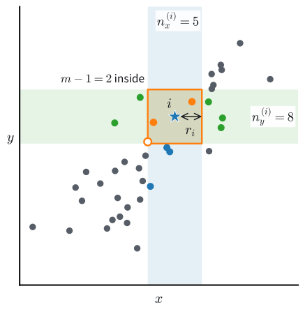
The estimator of Kraskov et al. (2004), KSG for short, replaces fixed cells by neighborhoods. Distances are measured by the largest coordinate difference (the Chebyshev distance), so a ball is a square in the plane and a box in higher dimension. Around sample \(i\) draw the smallest box in the joint \((x, y)\) space that reaches its \(m\)-th nearest neighbor, and call its half-width \(r_i\). The box holds the fraction \(m/n\) of the \(n\) samples, an estimate of the joint probability near the point. The strip \(|x - x_i| < r_i\) of the same half-width holds \(n_x^{(i)}\) other samples and the strip \(|y - y_i| < r_i\) holds \(n_y^{(i)}\); their fractions estimate the two marginal probabilities. The logarithm of the joint fraction over the product of the marginal fractions is a pointwise mutual information computed by counting. Figure 28.5.1 shows the three counts at one point.
Averaging these local log ratios, with the digamma function \(\psi = (\log \Gamma)'\) in place of the logarithm to remove the bias of small counts, gives the estimator
\[\hat{I}_{\textrm{KSG}} = \psi(m) + \psi(n) - \frac{1}{n} \sum_{i=1}^{n} \left(\psi\left(n_x^{(i)} + 1\right) + \psi\left(n_y^{(i)} + 1\right)\right). \tag{28.5.3}\]
Since \(\psi(j) \approx \log j\) for large \(j\), each summand is approximately \(\log\frac{m/n}{(n_x^{(i)}/n)(n_y^{(i)}/n)}\), the box fraction over the product of the strip fractions. The radii \(r_i\) adapt to the data, so there is no bin width or bandwidth to choose. Both strip counts use the strict inequality and exclude the point itself.
How do we count the neighbors of all points at once? The function computes the \(n \times n\) matrices of Chebyshev distances in each space with cdist; the joint distance is their elementwise maximum, because the largest coordinate difference of \((x, y)\) is the larger of the two largest differences.
def ksg_mi(x, y, m=5):
    """KSG nearest-neighbor estimate of I(X;Y) in nats; x, y are (n, d)."""
    n = len(x)
    dx, dy = cdist(x, x, 'chebyshev'), cdist(y, y, 'chebyshev')
    d = np.maximum(dx, dy)                       # joint Chebyshev distance
    np.fill_diagonal(d, np.inf)
    r = np.sort(d, axis=1)[:, m - 1]             # half-width: m-th neighbor
    n_x = (dx < r[:, None]).sum(axis=1) - 1      # strict, self excluded
    n_y = (dy < r[:, None]).sum(axis=1) - 1
    return float(digamma(m) + digamma(n)
                 - (digamma(n_x + 1) + digamma(n_y + 1)).mean())
How large can the estimate be? Each summand of Equation 28.5.3 involves only counts, so counting alone bounds it.
Proposition (sample-size ceiling of KSG). For any sample of \(n\) points in which no two joint distances from the same point are equal,
\[\hat{I}_{\textrm{KSG}} \leq \psi(n) - \psi(m), \tag{28.5.4}\]
with equality when \(Y = X\).
Proof. Without ties, exactly \(m - 1\) samples lie strictly closer to point \(i\) than its \(m\)-th neighbor. Each of them satisfies \(|x_j - x_i| < r_i\) and \(|y_j - y_i| < r_i\), because the joint distance is the larger of the two coordinate distances, so it lies in both strips: \(n_x^{(i)} \geq m - 1\) and \(n_y^{(i)} \geq m - 1\). The digamma function is increasing, so each summand is at most \(\psi(m) + \psi(n) - 2\psi(m) = \psi(n) - \psi(m)\). For \(Y = X\) the three distances coincide, both strips hold exactly the \(m - 1\) points inside the box, and every summand attains the bound. \(\blacksquare\)
At \(n = 2{,}000\) and \(m = 5\) the ceiling is \(\psi(2000) - \psi(5) = 6.09\) nats, close to \(\log(n/m) = 5.99\). A pair with infinite information, \(Y = X\) for continuous \(X\), is reported as \(6.1\) nats, and doubling the sample raises the ceiling by only about \(\log 2\). Counting neighbors can certify only as much information as the sample has distinguishable neighborhoods, about \(n/m\) of them. This is the first ceiling of the section, and every later one has the same shape: an estimator cannot report more than the logarithm of the number of things it can tell apart.
28.5.1.3 KSG in High Dimension
Does the estimator keep its accuracy in more dimensions? Take \(d\) independent copies of the pair, each with \(\rho = 0.9\), so that \(X\) and \(Y\) are \(d\)-dimensional. Information adds over independent coordinates: the joint density and the product of the marginals both factorize over the copies, so the log ratio is a sum of \(d\) terms, and the truth is \(d \times 0.83\) nats. The cell also runs \(Y = X\), which attains the ceiling.
n, rho = 2000, 0.9
for dim in (1, 4, 16):
    x, y = gauss_pair(rng, rho, (n, dim))        # dim independent pairs
    print(f'd = {dim:2d}: true I = {dim * mi_gauss(rho):6.2f}, '
          f'KSG = {ksg_mi(x, y):5.2f} nats')
x = rng.standard_normal((n, 1))
print(f'Y = X:  KSG = {ksg_mi(x, x):.2f}, '
f'ceiling psi(n) - psi(m) = {digamma(n) - digamma(5):.2f} nats')d = 1: true I = 0.83, KSG = 0.83 nats
d = 4: true I = 3.32, KSG = 2.51 nats
d = 16: true I = 13.29, KSG = 2.81 nats
Y = X: KSG = 6.09, ceiling psi(n) - psi(m) = 6.09 natsd = 1: true I = 0.83, KSG = 0.83 nats
d = 4: true I = 3.32, KSG = 2.45 nats
d = 16: true I = 13.29, KSG = 2.79 nats
Y = X: KSG = 6.09, ceiling psi(n) - psi(m) = 6.09 natsd = 1: true I = 0.83, KSG = 0.85 nats
d = 4: true I = 3.32, KSG = 2.51 nats
d = 16: true I = 13.29, KSG = 2.77 nats
Y = X: KSG = 6.09, ceiling psi(n) - psi(m) = 6.09 natsd = 1: true I = 0.83, KSG = 0.85 nats
d = 4: true I = 3.32, KSG = 2.55 nats
d = 16: true I = 13.29, KSG = 2.82 nats
Y = X: KSG = 6.09, ceiling psi(n) - psi(m) = 6.09 natsIn one dimension KSG lands within about \(0.1\) nat of the truth, and it does as well in two (the cell does not print that case). At \(d = 4\) it reports about \(2.5\) for \(3.3\), almost a nat low. At \(d = 16\) it reports \(2.8\) for \(13.3\): below even its \(6.1\)-nat ceiling, and about what it reports at \(d = 8\). The estimator has saturated: its output no longer grows with the information.
The cause is that the neighborhoods stop being local. A box that holds a fraction \(m/n\) of a roughly uniform sample in \(2d\) dimensions has sides about \((m/n)^{1/(2d)}\) times the width of the data: \(0.05\) at \(d = 1\), but \(0.83\) at \(d = 16\). The estimator assumes that the density is nearly constant over each box, and a box that spans most of the data violates that assumption. The strip counts show the effect. They hold about \(70\) of the \(2{,}000\) points at \(d = 1\), about \(31\) at \(d = 4\), and about \(26\) at both \(d = 8\) and \(d = 16\), although the truth doubles between the last two (3). The smoothness that makes neighbor counts consistent needs a sample that grows exponentially with the dimension.
28.5.1.4 Limits of Distribution-Free Estimation
Perhaps a cleverer estimator does better. Ask only for a lower bound: a function \(B\) of \(n\) samples such that \(B \leq I(X; Y)\) with probability at least \(1 - \delta\) for every distribution of the pair, with failure probability \(\delta < \tfrac{1}{2}\). Lower bounds are the useful direction, because a representation learner wants to certify that two views share a lot.
The smallest case shows the obstacle. Let \(Y = X\) be a copy of a discrete variable, so that \(I(X; Y) = H(X)\), and let \(X\) be uniform on \(M\) symbols. Draw \(n\) samples. Two given samples coincide with probability \(1/M\), so by the union bound over the \(n(n-1)/2\) pairs some two coincide with probability at most \(n(n-1)/(2M)\). Suppose that \(B\) looks only at which values repeat in the sample (its type), as must any estimator that treats the symbols as labels without meaning. With \(M = n^2\) the sample consists of \(n\) distinct values with probability more than \(\tfrac{1}{2}\), and \(B \leq \log n^2\) holds with probability at least \(1 - \delta > \tfrac{1}{2}\). The two events overlap, so \(B \leq 2 \log n\) on some all-distinct sample. All such samples have the same type, so \(B\) reports at most \(2 \log n\) on every sample of \(n\) distinct values, whatever source produced it.
Now take \(M = 2^{256}\) symbols, entropy \(256 \ln 2 = 177\) nats. At \(n = 10^6\) the sample is all distinct with probability at least \(1 - 4.3 \times 10^{-66}\), and on that sample \(B\) reports at most \(2 \log 10^6 = 27.6\) nats. A million samples cannot certify \(177\) nats, and they cannot certify \(30\). 6 works through the proof.
McAllester and Stratos (2020) proved the general statement, without the assumption on types:
Theorem (McAllester–Stratos, informal). Any distribution-free lower bound on \(I(X; Y)\) that holds with fixed confidence from \(n\) samples is \(O(\log n)\).
The reparameterization invariance of the previous section is part of the reason: mutual information does not change under an invertible relabelling of either variable, so an estimator must cope with every relabelling of the sample at once, and all it can rely on is which values repeat. Any estimator that reports more than the logarithm of its sample size does so by assuming something: smoothness, as KSG does, or a model family, as the bounds that follow do.
28.5.2 Variational Lower Bounds
Mutual information is an expectation of \(\log\frac{p(x, y)}{p(x)\,p(y)}\), and the densities in it are unknown. Variational methods replace them by an auxiliary model, a decoder that predicts one variable from the other or a critic that scores pairs. The model is chosen so that the result is a lower bound on the information for every model, and optimizing the model tightens the bound. One estimation problem becomes an optimization problem, and the result carries the model’s approximation error and the finite-sample error. Contrastive methods use the resulting bound as their training objective. Poole et al. (2019) give a unified treatment. Every proof below rests on Gibbs’ inequality from the first section of this chapter: the KL divergence \(D_{\textrm{KL}}(P \| Q)\) is nonnegative and is zero only when the two distributions agree.
28.5.2.1 The Barber–Agakov Bound
The first bound replaces the unknown posterior \(p(x \mid y)\) by a model of it.
Proposition (Barber–Agakov bound). For any conditional density \(q(x \mid y)\),
\[I(X; Y) \geq H(X) + \mathbb{E}_{(x,y) \sim P_{X,Y}}\left[\log q(x \mid y)\right], \tag{28.5.5}\]
with equality if and only if \(q(x \mid y) = p(x \mid y)\). For continuous \(X\) the differential entropy \(h(X)\) takes the place of \(H(X)\).
Proof. Write \(I(X; Y) = H(X) - H(X \mid Y)\) and insert the model:
\[ I(X; Y) - H(X) - \mathbb{E}\left[\log q(x \mid y)\right] = \mathbb{E}\left[\log \frac{p(x \mid y)}{q(x \mid y)}\right] = \mathbb{E}_{y}\left[D_{\textrm{KL}}\big(p(\cdot \mid y) \,\|\, q(\cdot \mid y)\big)\right] \geq 0 \]
by Gibbs’ inequality, applied for each value of \(y\) and averaged. Equality holds if and only if every divergence vanishes, that is, when \(q\) is the posterior. \(\blacksquare\)
The bound (Barber and Agakov 2003) is the information-theoretic reading of an encoder–decoder: if a decoder reconstructs \(X\) from \(Y\) with low cross-entropy, the pair must share a lot of information. Its weak point is \(H(X)\), which is unknown in the situations where we need the bound. It is a constant, however, so maximizing the bound over \(q\) never needs it. Substituting \(H(X) = -\mathbb{E}\log p(x)\) gives the equivalent ratio form \(I(X; Y) \geq \mathbb{E}\left[\log \left(q(x \mid y)/p(x)\right)\right]\), which InfoNCE will use.
Two instances show what the bound certifies. First, exchange the roles of the variables, which is allowed because \(I\) is symmetric, and let \(q(y \mid x)\) be the softmax of a classifier over \(k\) balanced classes, so that \(H(Y) = \log k\) and \(-\mathbb{E}\log q(y \mid x) = L\) is its held-out cross-entropy. Then
\[I(X; Y) \geq \log k - L. \tag{28.5.6}\]
A 10-class model with held-out cross-entropy \(0.3\) certifies \(\ln 10 - 0.3 = 2.0\) nats of label information, and since \(L \geq 0\), no classifier certifies more than \(\ln 10 = 2.30\). InfoNCE will have this shape. Second, for the Gaussian pair, a decoder trained by squared error alone is a Gaussian \(q(x \mid y) = \mathcal{N}(x; a y, 1)\) with unit variance. With \(h(X) = \tfrac{1}{2}\log(2\pi e)\) the bound becomes \(\tfrac{1}{2} - \tfrac{1}{2}\mathbb{E}(X - aY)^2 = \tfrac{1}{2} - \tfrac{1}{2}(1 - 2a\rho + a^2)\), which is largest at \(a = \rho\), where it equals \(\rho^2/2\). At \(\rho = 0.9\) this decoder certifies \(0.41\) nats of the true \(0.83\), and it never certifies more than \(\tfrac{1}{2}\) however strong the dependence. The gap is the bias of a decoder whose variance is fixed at \(1\) instead of the true conditional variance \(1 - \rho^2\) (4).
28.5.2.2 The Donsker–Varadhan Bound
The second bound needs neither a normalized model nor \(H(X)\). It writes the KL divergence, and hence mutual information, as a supremum over arbitrary critic functions \(T\), with no requirement that anything integrate to one. This is the convex-duality pattern behind the f-GAN construction of Section 28.3.
Proposition (Donsker–Varadhan representation). For distributions \(P\) and \(Q\) and any function \(T\) with \(\mathbb{E}_Q[e^T] < \infty\),
\[D_{\textrm{KL}}(P \| Q) \geq \mathbb{E}_P[T] - \log \mathbb{E}_Q\left[e^{T}\right], \tag{28.5.7}\]
with equality if and only if \(T = \log \frac{dP}{dQ} + c\) for a constant \(c\); when \(P \ll Q\) and the divergence is finite, the supremum over \(T\) attains \(D_{\textrm{KL}}(P \| Q)\) (Donsker and Varadhan 1983).
Proof. If \(P\) is not absolutely continuous with respect to \(Q\), the left side is infinite. Otherwise, given \(T\), define the Gibbs distribution \(\tilde{Q}\) with density \(\tilde{q}(x) = q(x)\, e^{T(x)} / Z\) and normalizer \(Z = \mathbb{E}_Q[e^T]\): the distribution \(Q\) tilted by the critic. Then
\[ D_{\textrm{KL}}(P \| Q) - \left(\mathbb{E}_P[T] - \log Z\right) = \mathbb{E}_P\left[\log \frac{p}{q} - T + \log Z\right] = \mathbb{E}_P\left[\log \frac{p}{\tilde{q}}\right] = D_{\textrm{KL}}(P \| \tilde{Q}) \geq 0, \]
by Gibbs’ inequality. Equality holds if and only if \(P = \tilde{Q}\), which means \(p/q = e^{T}/Z\), or \(T = \log(p/q) + \log Z\). \(\blacksquare\)
The gap of the bound is the divergence from \(P\) to the tilted distribution, so a critic is good when tilting \(Q\) by \(e^T\) reproduces \(P\). Specializing to \(P = P_{X,Y}\) and \(Q = P_X \otimes P_Y\) bounds mutual information: for any critic \(T(x, y)\),
\[ I(X; Y) \geq \mathbb{E}_{P_{X,Y}}[T] - \log \mathbb{E}_{P_X \otimes P_Y}\left[e^{T}\right]. \]
The first expectation is an average over the sample pairs. The second needs pairs with no dependence, and the code obtains them by pairing each \(x\) with the \(y\) of a different sample, a single roll of the batch, as in the running-example cell. MINE (mutual information neural estimation, Belghazi et al. (2018)) is this bound with a neural network as the critic; its gradient uses a moving average of \(\mathbb{E}_Q[e^T]\) across minibatches, because the minibatch gradient of the logarithm of an average is biased.
28.5.2.3 The NWJ Bound
The logarithm in front of \(\mathbb{E}_Q[e^T]\) couples all the samples of a batch, and it biases the minibatch estimate. By Jensen’s inequality the logarithm of a batch average is on average below the logarithm of the population average, so the minibatch DV value \(\overline{T} - \log \overline{e^T}\) overestimates the bound in expectation. The tangent-line inequality \(\log z \leq z/e\), with equality at \(z = e\), removes the logarithm: applied to \(Z = \mathbb{E}_Q[e^T]\) in Equation 28.5.7, it gives, for every critic \(T\),
\[I(X; Y) \geq \mathbb{E}_{P_{X,Y}}[T] - e^{-1}\, \mathbb{E}_{P_X \otimes P_Y}\left[e^{T}\right]. \tag{28.5.8}\]
This is the NWJ bound (Nguyen et al. 2010), and it is tight at \(T^* = 1 + \log\frac{dP}{dQ}\), the critic for which \(Z = e\). Since \(e^{-1}\, \mathbb{E}_Q[e^T] = \mathbb{E}_Q[e^{T-1}]\), it is the f-GAN bound on the KL divergence, \(D_{\textrm{KL}}(P \| Q) \geq \mathbb{E}_P[T] - \mathbb{E}_Q[e^{T-1}]\), that Section 28.3 derived from the convex conjugate of \(u \log u\). Because no logarithm of an average appears, the minibatch value of Equation 28.5.8 is an unbiased estimate of the bound. The term \(e^T\) has a different problem. For the optimal critic, \(e^{T^*-1}\) is the density ratio, which is enormous on rare pairs and tiny on typical ones, so its average over a batch is dominated by pairs that most batches do not contain. With an exact critic, a typical batch therefore overshoots the bound and a rare batch undershoots it by a lot; Section 28.5.3.4 measures both.
28.5.3 InfoNCE
28.5.3.1 The Contrastive Loss
The \(e^T\) of the DV and NWJ bounds is unnormalized, so a single pair can dominate a batch. InfoNCE normalizes it within the batch: it makes the candidates compete. Draw one positive pair \((x, y^+) \sim P_{X,Y}\) and \(N - 1\) negatives \(y_2, \ldots, y_N\) drawn independently from \(P_Y\). Score every candidate with the critic \(T(x, y)\), and ask a softmax over the \(N\) scores to point at the positive. The InfoNCE loss (Oord et al. 2018) is the resulting cross-entropy,
\[\mathcal{L}_{\textrm{NCE}} = -\mathbb{E}\left[\log \frac{e^{T(x, y^+)}}{e^{T(x, y^+)} + \sum_{j=2}^{N} e^{T(x, y_j)}}\right], \tag{28.5.9}\]
where the expectation is over the positive pair and the negatives. The associated estimate of mutual information is the logarithm of the number of candidates minus the loss,
\[\hat{I}_{\textrm{NCE}} = \log N - \mathcal{L}_{\textrm{NCE}}. \tag{28.5.10}\]
Many papers, following Oord et al. (2018), write the loss with a \(\frac{1}{N}\) inside the logarithm and a compensating \(\log N\) outside; the two conventions give the same number. The loss is an \(N\)-class cross-entropy whose classes are the other examples in the batch rather than fixed labels. It is the loss of CPC, SimCLR and CLIP (Oord et al. 2018; Chen et al. 2020; Radford et al. 2021), where \(x\) and \(y\) are two views or two modalities of one example and the batch supplies the negatives.

Figure 28.5.2 shows the game. Its smallest case is \(N = 2\): one negative, and the loss is the binary cross-entropy of telling the true partner from an impostor. Even a perfect answer shows only that one of two candidates was right, and the estimate is at most \(\ln 2 = 0.69\) nats.
28.5.3.2 The InfoNCE Bound
The proposition says that a small loss certifies information, and that the certificate is capped (Poole et al. 2019).
Proposition (InfoNCE bound). For any measurable critic \(T\) and any \(N \geq 1\),
\[I(X; Y) \geq \log N - \mathcal{L}_{\textrm{NCE}}. \tag{28.5.11}\]
The right-hand side is at most \(\log N\).
Proof. Number the candidates \(y_1 = y^+, y_2, \ldots, y_N\) and write \(V = (Y_1, \ldots, Y_N)\) for the whole bag. The negatives \(Y_{2:N}\) are independent of the pair \((X, Y_1)\). The proof replaces \(Y\) by the bag, finds a normalized model of the bag given \(X\), and applies Barber–Agakov.
Step 1: independent negatives add no information. The chain rule of the previous section splits the information in the bag, \(I(X; Y_1, Y_{2:N}) = I(X; Y_1) + I(X; Y_{2:N} \mid Y_1)\). Given \(Y_1\), the negatives are still independent of \(X\), because they are independent of \((X, Y_1)\); the second term is therefore \(0\), and \(I(X; V) = I(X; Y)\).
Step 2: the softmax ratio is a normalized model. This is the step that is not routine. Define
\[ \gamma(x, v) = \frac{e^{T(x, y_1)}}{\frac{1}{N}\sum_{j=1}^N e^{T(x, y_j)}}, \]
which lies between \(0\) and \(N\). Let \(p(v)\) be the distribution of a bag of \(N\) independent draws from \(P_Y\), the positive slot included. The \(N\) candidates of such a bag are exchangeable, so the \(N\) ratios \(e^{T(x, y_i)} / \frac{1}{N}\sum_j e^{T(x, y_j)}\) have the same expectation, and for every fixed \(x\)
\[ \mathbb{E}_{p(v)}\left[\gamma(x, V)\right] = \frac{1}{N}\sum_{i=1}^{N} \mathbb{E}_{p(v)}\left[\frac{e^{T(x, Y_i)}}{\frac{1}{N}\sum_{j} e^{T(x, Y_j)}}\right] = \mathbb{E}_{p(v)}\left[\frac{\frac{1}{N}\sum_{i} e^{T(x, Y_i)}}{\frac{1}{N}\sum_{j} e^{T(x, Y_j)}}\right] = 1. \]
Hence \(q(v \mid x) = p(v)\, \gamma(x, v)\) is a conditional distribution over bags.
Step 3: Barber–Agakov on the bag. Apply the ratio form of Equation 28.5.5 to the pair \((X, V)\) with the model \(q(v \mid x)\), the two variables’ roles exchanged, which the symmetry of \(I\) allows:
\[ I(X; V) \geq \mathbb{E}_{p(x, v)}\left[\log \frac{q(v \mid x)}{p(v)}\right] = \mathbb{E}\left[\log \gamma(X, V)\right] = \log N - \mathcal{L}_{\textrm{NCE}}. \]
The last equality holds because \(\log \gamma\) is \(\log N\) plus the log-softmax probability of the positive. With Step 1 this proves the bound. The softmax probability of the positive is at most \(1\), so \(\mathcal{L}_{\textrm{NCE}} \geq 0\) and the right-hand side is at most \(\log N\). \(\blacksquare\)
Naming the right partner out of \(N\) candidates, even with certainty, demonstrates \(\log N\) nats, the information in one choice among \(N\); no critic can make the game show more. The loss is smallest for the critics \(T^*(x, y) = \textrm{pmi}(x, y) + c(x)\), with any function \(c\) of the anchor alone (7). A larger \(N\) raises the ceiling, which is one reason CPC, SimCLR and CLIP use large batches.
28.5.3.3 The Ceiling with an Exact Critic
With the exact critic \(T = \textrm{pmi}\), how does the estimate depend on the true information and on \(N\)? The cell scores all \(N \times N\) pairs of a batch at once: row \(i\) holds anchor \(x_i\) against every \(y_j\), its diagonal entry is the positive, and the other \(N - 1\) entries are its negatives. It then sweeps the true information for \(N = 16\), \(128\) and \(1024\), with dotted lines at the three ceilings \(\ln N\).
def infonce_bound(f):
    """log N minus the InfoNCE loss of an N x N score matrix f[i, j]."""
    return np.log(len(f)) + np.mean(np.diag(f) - logsumexp(f, axis=1))

def exact_scores(x, y, rho):
    """The exact critic T = pmi on all N x N pairs (x_i, y_j) of a batch."""
    return pmi_gauss(x[:, None], y[None, :], rho)

true_mi = np.array([0.25, 0.5, 1, 1.5, 2, 2.5, 3, 4, 5, 6, 7])
rhos = np.sqrt(1 - np.exp(-2 * true_mi))                 # invert mi_gauss
Ns = (16, 128, 1024)
ests = [[np.mean([infonce_bound(exact_scores(*gauss_pair(rng, r, N), r))
                  for _ in range(200 if N <= 128 else 50)]) for r in rhos]
        for N in Ns]
d2l.plot(true_mi, ests + [true_mi] + [[np.log(N)] * len(true_mi) for N in Ns],
         'true I(X;Y) (nats)', 'InfoNCE estimate (nats)',
         legend=[f'N = {N}' for N in Ns] + ['truth'],
         fmts=('-', '-', '-', 'k--', 'k:', 'k:', 'k:'), figsize=(5, 3))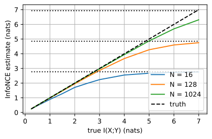
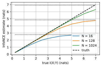
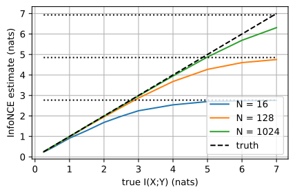
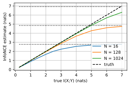
Each curve leaves the diagonal early and smoothly, not at its ceiling. At \(I = 4\) the \(N = 128\) curve reads \(3.7\), although its ceiling is \(4.85\); at \(I = 6\) it reads \(4.6\); and at \(I = 7\) the \(N = 1024\) curve reads \(6.3\) against a ceiling of \(6.93\). Inserting \(T = \textrm{pmi}\) into the loss shows where the gap comes from:
\[\hat{I}_{\textrm{NCE}} = I(X; Y) - \mathbb{E}\left[\log \frac{1}{N}\sum_{j=1}^N e^{\textrm{pmi}(x, y_j)}\right]. \tag{28.5.12}\]
The correction is the bound’s own slack, and it is nonnegative by the proposition. Its average contains the positive’s own term \(e^{\textrm{pmi}(x, y^+)}/N\), so the correction is at least \(\mathbb{E}[\textrm{pmi}(x, y^+)] - \log N = I - \log N\), which is the cap again. The other \(N - 1\) terms average to about \(1\) only when \(N\) is large enough to contain the rare negatives that carry \(\mathbb{E}[e^{\textrm{pmi}}] = 1\), so the slack vanishes only as \(N \to \infty\) (7). The cap is the crudest consequence of this slack.
Fano’s inequality of the previous section turns the cap into a requirement. Features that predict one of \(k\) balanced classes with error probability \(P_e\) must share at least \(\log k - H_b(P_e) - P_e \log(k - 1)\) nats with the label, where \(H_b\) is the binary entropy; \(5\%\) error on \(1{,}000\) classes needs \(6.36\) nats. An InfoNCE bound between the features and the label can certify that much only with \(N \geq e^{6.36} \approx 581\) candidates, and, if its slack behaves like that of the Gaussian curves above, only with more than a thousand: the \(N = 1024\) curve reaches \(6.3\) only when the truth is \(7\).
28.5.3.4 Exact Critics Compared
At \(N = 128\), with the exact critic \(T^* = 1 + \textrm{pmi}\) for all three bounds (adding a constant does not change InfoNCE), how do the batch values of DV, NWJ and InfoNCE behave as the true information grows? The cell draws \(200\) batches at each level and prints the median and the quartiles of the batch values, and the mean for NWJ. With heavy tails, quartiles describe the spread better than a standard deviation does. The plot draws the medians as solid lines and the quartiles as dotted lines of the same colour. The product expectations use the rolled batch, and the DV logarithm of an average is computed with logsumexp so that it cannot underflow.
def quartiles(a):
    """Median and quartiles of a list of batch values, as text."""
    q1, med, q3 = np.percentile(a, [25, 50, 75])
    return f'{med:5.2f} [{q1:5.2f}, {q3:5.2f}]'

N, true_mi = 128, np.array([0.5, 1, 2, 3, 4, 5, 6])
medians, quarts = [], []
print(f'{"I":>3}  {"DV median [IQR]":20}  {"NWJ median [IQR]":20}  '
      f'{"NWJ mean":>8}  {"InfoNCE median [IQR]":20}')
for I in true_mi:
    rho, dv, nwj, nce = np.sqrt(1 - np.exp(-2 * I)), [], [], []
    for _ in range(200):
        x, y = gauss_pair(rng, rho, N)
        T_joint = 1 + pmi_gauss(x, y, rho)               # T* on true pairs
        T_prod = 1 + pmi_gauss(x, np.roll(y, 1), rho)    # T* on mismatched
        dv.append(T_joint.mean() - (logsumexp(T_prod) - np.log(N)))
        nwj.append(T_joint.mean() - np.exp(T_prod - 1).mean())
        nce.append(infonce_bound(exact_scores(x, y, rho)))
    medians.append([np.median(a) for a in (dv, nwj, nce)])
    quarts.append([np.percentile(a, q) for a in (dv, nwj, nce) for q in (25, 75)])
    print(f'{I:3.1f}  {quartiles(dv)}  {quartiles(nwj)}  {np.mean(nwj):8.2f}'
          f'  {quartiles(nce)}')
d2l.plot(true_mi, list(np.array(medians).T) + [true_mi, [np.log(N)] * 7]
         + list(np.array(quarts).T), 'true I(X;Y) (nats)', 'batch value (nats)',
         legend=['DV', 'NWJ', 'InfoNCE', 'truth'], ylim=[0, 8],
         fmts=('C0-', 'C1-', 'C2-', 'k--', 'k:', 'C0:', 'C0:', 'C1:', 'C1:',
'C2:', 'C2:'), figsize=(5, 3)) I DV median [IQR] NWJ median [IQR] NWJ mean InfoNCE median [IQR]
0.5 0.50 [ 0.42, 0.59] 0.50 [ 0.42, 0.59] 0.50 0.50 [ 0.45, 0.55]
1.0 1.03 [ 0.89, 1.16] 1.02 [ 0.89, 1.15] 1.02 0.99 [ 0.94, 1.04]
2.0 2.02 [ 1.82, 2.17] 2.02 [ 1.81, 2.16] 1.98 1.95 [ 1.89, 2.01]
3.0 3.00 [ 2.71, 3.39] 2.99 [ 2.66, 3.33] 2.93 2.88 [ 2.80, 2.92]
4.0 4.18 [ 3.72, 4.84] 4.16 [ 3.69, 4.56] 3.93 3.67 [ 3.62, 3.72]
5.0 5.79 [ 4.83, 9.38] 5.53 [ 4.79, 5.92] 5.21 4.26 [ 4.22, 4.32]
6.0 11.66 [ 5.91, 32.15] 6.90 [ 5.90, 7.01] 6.04 4.60 [ 4.56, 4.64]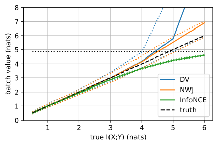
  I  DV median [IQR]       NWJ median [IQR]      NWJ mean  InfoNCE median [IQR]
0.5   0.52 [ 0.44,  0.60]   0.51 [ 0.44,  0.60]      0.52   0.50 [ 0.45,  0.54]
1.0   1.02 [ 0.92,  1.13]   1.02 [ 0.91,  1.13]      1.01   0.99 [ 0.95,  1.04]
2.0   2.06 [ 1.86,  2.25]   2.05 [ 1.85,  2.22]      2.03   1.96 [ 1.90,  2.02]
3.0   3.08 [ 2.78,  3.40]   3.08 [ 2.73,  3.32]      3.01   2.86 [ 2.81,  2.92]
4.0   4.15 [ 3.71,  4.82]   4.13 [ 3.66,  4.57]      4.02   3.68 [ 3.63,  3.73]
5.0   5.42 [ 4.56,  8.51]   5.34 [ 4.43,  5.91]      4.99   4.28 [ 4.23,  4.32]
6.0  11.24 [ 5.93, 32.41]   6.92 [ 5.92,  7.02]      6.04   4.61 [ 4.57,  4.64]
  I  DV median [IQR]       NWJ median [IQR]      NWJ mean  InfoNCE median [IQR]
0.5   0.51 [ 0.44,  0.59]   0.50 [ 0.43,  0.58]      0.50   0.49 [ 0.44,  0.54]
1.0   1.00 [ 0.90,  1.12]   1.00 [ 0.89,  1.11]      1.00   0.99 [ 0.92,  1.04]
2.0   2.05 [ 1.80,  2.25]   2.04 [ 1.78,  2.23]      2.00   1.96 [ 1.90,  2.02]
3.0   3.01 [ 2.73,  3.32]   3.01 [ 2.68,  3.27]      2.96   2.85 [ 2.80,  2.93]
4.0   4.12 [ 3.70,  4.69]   4.12 [ 3.62,  4.50]      3.99   3.67 [ 3.62,  3.72]
5.0   5.56 [ 4.58,  9.28]   5.42 [ 4.46,  5.94]      5.03   4.28 [ 4.23,  4.33]
6.0  13.28 [ 5.69, 36.42]   6.93 [ 5.59,  7.02]      5.89   4.62 [ 4.58,  4.65]
  I  DV median [IQR]       NWJ median [IQR]      NWJ mean  InfoNCE median [IQR]
0.5   0.51 [ 0.43,  0.60]   0.51 [ 0.43,  0.59]      0.51   0.50 [ 0.45,  0.55]
1.0   1.04 [ 0.92,  1.15]   1.04 [ 0.91,  1.13]      1.02   0.99 [ 0.94,  1.05]
2.0   2.09 [ 1.84,  2.27]   2.09 [ 1.83,  2.24]      2.04   1.96 [ 1.91,  2.01]
3.0   3.12 [ 2.84,  3.44]   3.12 [ 2.83,  3.34]      3.07   2.88 [ 2.82,  2.93]
4.0   4.09 [ 3.70,  4.80]   4.09 [ 3.66,  4.58]      3.99   3.68 [ 3.63,  3.74]
5.0   5.77 [ 4.79,  8.37]   5.52 [ 4.76,  5.94]      5.18   4.27 [ 4.22,  4.32]
6.0  14.33 [ 6.28, 47.54]   6.92 [ 6.22,  7.01]      6.29   4.61 [ 4.58,  4.64]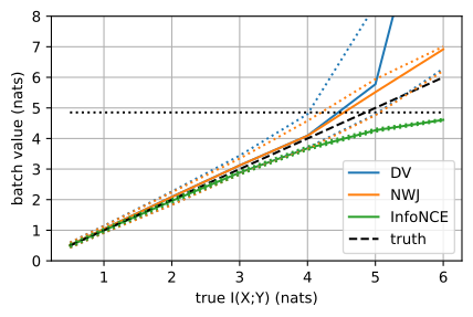
Up to \(I = 3\) the three medians are within about \(0.15\) nat of the truth, and InfoNCE has the narrowest spread (an interquartile range of about \(0.1\) nat, against \(0.15\) to \(0.7\) for the others). At \(I = 4\) the DV and NWJ medians are slightly above \(4\), and InfoNCE reads \(3.7\) under its cap of \(4.85\). At \(I = 6\) InfoNCE reads \(4.6\) with an interquartile range below \(0.1\). NWJ’s median is about \(7 = I + 1\), while its mean is usually within half a nat of \(6\). DV’s median lies several nats above the truth, with an upper quartile in the tens, so its curve leaves the plot. NWJ’s upper quartile at \(I = 6\) sits at \(I + 1\), on top of its median, so half of the batches overshoot by about a nat.
The rare pairs described in the NWJ subsection explain these numbers. The product expectation \(\mathbb{E}_Q[e^{\textrm{pmi}}] = 1\) is carried by the rare independent pairs that happen to look like partners. At \(I = 6\) the typical batch’s average of \(e^{\textrm{pmi}}\) over its \(128\) mismatched pairs is near zero (its median over batches is at most a few hundredths, and more than half of the batches stay below \(0.1\)). On such a batch NWJ reports \(\mathbb{E}_P[T^*] - 0 = 1 + I\), one nat high, and DV reports the average pmi minus the logarithm of a near-zero average, many nats high. About one batch in four holds a single mismatched pair with \(e^{\textrm{pmi}} \geq N\), which alone pulls NWJ down by a nat or more. Such batches, and rarer ones that pull it down much further, hold NWJ’s mean at the truth and make its variance enormous. The mismatched-pair term has variance \((e^{2I} - 1)/N\), a standard deviation of \(36\) nats at \(I = 6\), carried by batches so rare that \(200\) draws seldom include one (2). InfoNCE normalizes within the batch, so a negative that looks like a partner costs at most one wrong softmax, never a factor \(e^{\textrm{pmi}}\).
The population DV and NWJ bounds are valid. The minibatch DV estimate is not a lower bound even in expectation, because of the logarithm of an average. The minibatch NWJ estimate is unbiased for its bound but dominated by rare batches. The minibatch InfoNCE estimate is steady, below the truth even with an exact critic, and at most \(\log N\).
28.5.3.5 Training a Critic
In practice the critic is learned. When a contrastive loss reports less than the truth, is the critic at fault, or the bound? We train a critic of the dual-encoder form that CLIP and SimCLR use: two small networks \(g, h : \mathbb{R} \to \mathbb{R}^{16}\) embed \(x\) and \(y\), and the critic is the inner product \(T(x, y) = g(x)^\top h(y)\). The \(N \times N\) score matrix of a batch is then one matrix product of the two embedding matrices, so \(N\) anchors against \(N\) candidates cost \(2N\) network evaluations instead of \(N^2\). The data are two disjoint pools of \(4{,}096\) pairs at \(\rho = 0.99\), one for training and one for evaluation; the true information is \(1.96\) nats.
rho, n_pool = 0.99, 4096
x_tr, y_tr = (a.astype(np.float32) for a in gauss_pair(rng, rho, n_pool))
x_ev, y_ev = (a.astype(np.float32) for a in gauss_pair(rng, rho, n_pool))
Each encoder is a multilayer perceptron with two hidden layers of \(64\) ReLU units and Glorot-uniform initialization. The loss is the InfoNCE loss of the score matrix, a cross-entropy whose label for row \(i\) is \(i\), the index of the positive; every framework has it as its standard classification loss.
def encoder(d_out=16, hidden=64):
    """An MLP that embeds a scalar in d_out dimensions."""
    net = torch.nn.Sequential(torch.nn.Linear(1, hidden), torch.nn.ReLU(),
                              torch.nn.Linear(hidden, hidden), torch.nn.ReLU(),
                              torch.nn.Linear(hidden, d_out))
    for layer in net[::2]:                          # the Linear layers
        torch.nn.init.xavier_uniform_(layer.weight)
        torch.nn.init.zeros_(layer.bias)
    return net

def scores(g, h, x, y):
    """All N x N critic values T(x_i, y_j) = g(x_i) . h(y_j)."""
    return g(x[:, None]) @ h(y[:, None]).T

def infonce_loss(f):
    """Cross-entropy of each row's softmax at its positive, the diagonal."""
    return torch.nn.functional.cross_entropy(f, torch.arange(len(f)))

g, h = encoder(), encoder()
def encoder(d_out=16, hidden=64):
"""An MLP that embeds a scalar in d_out dimensions."""
return tf.keras.Sequential([
tf.keras.Input((1,)), tf.keras.layers.Dense(hidden, activation='relu'),
tf.keras.layers.Dense(hidden, activation='relu'),
tf.keras.layers.Dense(d_out)])
def scores(g, h, x, y):
"""All N x N critic values T(x_i, y_j) = g(x_i) . h(y_j)."""
return tf.matmul(g(x[:, None]), h(y[:, None]), transpose_b=True)
def infonce_loss(f):
"""Cross-entropy of each row's softmax at its positive, the diagonal."""
return tf.reduce_mean(tf.keras.losses.sparse_categorical_crossentropy(
tf.range(tf.shape(f)[0]), f, from_logits=True))
g, h = encoder(), encoder()def init_encoder(key, sizes=(1, 64, 64, 16)):
"""Glorot-uniform weights and zero biases of an MLP with these widths."""
glorot = jax.nn.initializers.glorot_uniform()
keys = jax.random.split(key, len(sizes) - 1)
return [(glorot(k, (a, b)), jnp.zeros(b))
for k, a, b in zip(keys, sizes[:-1], sizes[1:])]
def encode(params, x):
"""Embed each scalar of x with the MLP."""
z = x[:, None]
for W, b in params[:-1]:
z = jax.nn.relu(z @ W + b)
W, b = params[-1]
return z @ W + b
def scores(params, x, y):
"""All N x N critic values T(x_i, y_j) = g(x_i) . h(y_j)."""
params_g, params_h = params
return encode(params_g, x) @ encode(params_h, y).T
def infonce_loss(params, x, y):
"""Cross-entropy of each row's softmax at its positive, the diagonal."""
f = scores(params, x, y)
return optax.softmax_cross_entropy_with_integer_labels(
f, jnp.arange(len(f))).mean()
key_g, key_h = jax.random.split(jax.random.key(int(rng.integers(2**31))))
params = (init_encoder(key_g), init_encoder(key_h))def encoder(d_out=16, hidden=64):
"""An MLP that embeds a scalar in d_out dimensions."""
net = gluon.nn.HybridSequential()
net.add(gluon.nn.Dense(hidden, activation='relu'),
gluon.nn.Dense(hidden, activation='relu'), gluon.nn.Dense(d_out))
net.initialize(init.Xavier())
net.hybridize()
return net
def scores(g, h, x, y):
"""All N x N critic values T(x_i, y_j) = g(x_i) . h(y_j)."""
return mnp.dot(g(x.reshape(-1, 1)), h(y.reshape(-1, 1)).T)
cross_entropy = gluon.loss.SoftmaxCrossEntropyLoss()
def infonce_loss(f):
"""Cross-entropy of each row's softmax at its positive, the diagonal."""
return cross_entropy(f, mnp.arange(len(f))).mean()
g, h = encoder(), encoder()Training runs \(1{,}000\) Adam steps with learning rate \(10^{-3}\) on batches of \(N = 128\) pairs drawn from the training pool. Afterwards, critic_np evaluates the trained critic on NumPy arrays, so that one evaluation cell serves every framework.
opt = torch.optim.Adam([*g.parameters(), *h.parameters()], lr=1e-3)
N = 128
for step in range(1000):
    idx = rng.choice(n_pool, N, replace=False)
    loss = infonce_loss(scores(g, h, torch.tensor(x_tr[idx]),
                               torch.tensor(y_tr[idx])))
    opt.zero_grad()
    loss.backward()
    opt.step()

def critic_np(a, b):
    """The trained critic on NumPy inputs, as an N x N NumPy array."""
    with torch.inference_mode():
        return scores(g, h, torch.tensor(a), torch.tensor(b)).numpy()
opt = tf.keras.optimizers.Adam(1e-3)
params = g.trainable_variables + h.trainable_variables
@tf.function
def train_step(x, y):
with tf.GradientTape() as tape:
loss = infonce_loss(scores(g, h, x, y))
opt.apply_gradients(zip(tape.gradient(loss, params), params))
N = 128
for step in range(1000):
idx = rng.choice(n_pool, N, replace=False)
train_step(tf.constant(x_tr[idx]), tf.constant(y_tr[idx]))
def critic_np(a, b):
"""The trained critic on NumPy inputs, as an N x N NumPy array."""
return scores(g, h, tf.constant(a), tf.constant(b)).numpy()opt = optax.adam(1e-3)
state = opt.init(params)
@jax.jit
def train_step(params, state, x, y):
grads = jax.grad(infonce_loss)(params, x, y)
updates, state = opt.update(grads, state)
return optax.apply_updates(params, updates), state
N = 128
for step in range(1000):
idx = rng.choice(n_pool, N, replace=False)
params, state = train_step(params, state, x_tr[idx], y_tr[idx])
def critic_np(a, b):
"""The trained critic on NumPy inputs, as an N x N NumPy array."""
return np.asarray(scores(params, a, b))trainer = gluon.Trainer(
list(g.collect_params().values()) + list(h.collect_params().values()),
'adam', {'learning_rate': 1e-3})
N = 128
for step in range(1000):
idx = rng.choice(n_pool, N, replace=False)
with autograd.record():
loss = infonce_loss(scores(g, h, mnp.array(x_tr[idx]),
mnp.array(y_tr[idx])))
loss.backward()
trainer.step(1)
def critic_np(a, b):
"""The trained critic on NumPy inputs, as an N x N NumPy array."""
return scores(g, h, mnp.array(a), mnp.array(b)).asnumpy()Does the learned critic reproduce the exact one? The evaluation cell cuts the evaluation pool into disjoint batches of \(N\) pairs, for \(N\) from \(2\) to \(128\), and computes the InfoNCE bound of the learned critic and of the exact critic on the same batches.
def infonce_eval(score, x, y, N):
    """Mean InfoNCE bound over the disjoint batches of N pairs in (x, y)."""
    return np.mean([infonce_bound(score(x[i:i + N], y[i:i + N]))
                    for i in range(0, len(x), N)])

def exact_np(a, b):
    """The exact critic T = pmi on the evaluation pairs."""
    return exact_scores(a, b, rho)

print('   N   ln N   learned   exact')
for N_ev in (2, 8, 32, 128):
    print(f'{N_ev:4d}  {np.log(N_ev):5.2f}  '
          f'{infonce_eval(critic_np, x_ev, y_ev, N_ev):7.2f}  '
          f'{infonce_eval(exact_np, x_ev, y_ev, N_ev):6.2f}')
print(f'true I(X;Y) = {mi_gauss(rho):.2f} nats') N ln N learned exact
2 0.69 0.57 0.58
8 2.08 1.41 1.42
32 3.47 1.77 1.80
128 4.85 1.89 1.92
true I(X;Y) = 1.96 nats N ln N learned exact
2 0.69 0.55 0.56
8 2.08 1.38 1.41
32 3.47 1.71 1.76
128 4.85 1.81 1.87
true I(X;Y) = 1.96 nats N ln N learned exact
2 0.69 0.57 0.58
8 2.08 1.39 1.41
32 3.47 1.73 1.78
128 4.85 1.84 1.91
true I(X;Y) = 1.96 nats N ln N learned exact
2 0.69 0.57 0.57
8 2.08 1.39 1.41
32 3.47 1.76 1.78
128 4.85 1.87 1.90
true I(X;Y) = 1.96 natsThe learned critic matches the exact one to within a few hundredths of a nat at every \(N\): about \(0.57\) at \(N = 2\), \(1.4\) at \(N = 8\), \(1.75\) at \(N = 32\) and \(1.8\) to \(1.9\) at \(N = 128\). The gap to the true \(1.96\) nats belongs to the bound, and it closes only as \(N\) grows. At \(N = 8\) the ceiling \(\ln 8 = 2.08\) already exceeds the truth, so the shortfall of about \(0.55\) nat there is the slack of the bound, not its cap.
SimCLR-style systems use a different critic: they normalize the two embeddings \(z_x\) and \(z_y\) and divide their cosine similarity by a temperature \(\tau\), \(T(x, y) = \textrm{sim}(z_x, z_y)/\tau\) (Chen et al. 2020). Lowering \(\tau\) sharpens the softmax over the candidates and concentrates the loss on the hardest negatives, those that score closest to the positive. The temperature also caps the bound: a cosine lies in \([-1, 1]\), so a cosine critic certifies less than \(2/\tau\) nats whatever \(N\) is (5). The symbol and its role are those of the distillation temperature of Section 28.1.
A tighter bound does not mean a better representation. Tschannen et al. (2020) found that downstream quality correlates poorly with the tightness of the bound being maximized: looser bounds sometimes give better representations, and the critic architecture and the choice of views matter as much as the information. A contrastive loss is a capped lower bound on the information, and the objective should be judged by the representations it trains.
28.5.4 The Compression-Phase Debate
Estimation pitfalls have shaped a debate about deep learning itself. Shwartz-Ziv and Tishby (2017) binned the activations of each layer \(Z\) of ordinary classifiers during training and plotted the estimated pairs \(\big(I(X; Z), I(Y; Z)\big)\), with input \(X\) and label \(Y\). They reported a fast fitting phase, in which both informations rise, followed by a long compression phase, in which \(I(X; Z)\) falls while \(I(Y; Z)\) holds, and they proposed compression as the mechanism by which deep networks generalize. Saxe et al. (2018) found that the compression appears with saturating activations such as \(\tanh\), which push activations into the edge bins, and disappears with ReLU networks, which generalize just as well.
The binned estimate explains the discrepancy. In a deterministic network the binned layer is a function of the input, so \(H(Z_{\textrm{bin}} \mid X) = 0\) and the binned estimate is \(I(X; Z_{\textrm{bin}}) = H(Z_{\textrm{bin}}) - H(Z_{\textrm{bin}} \mid X) = H(Z_{\textrm{bin}})\), the entropy of a quantization of the layer. It is at most the logarithm of the number of inputs, \(\ln 4096 = 8.3\) nats in the original experiment. For continuous inputs and activations whose distribution has no atoms, the true \(I(X; Z)\) is infinite. The curves therefore track how the activations spread over the bins, which saturating units change as they move into the edge bins (10).
We can now name the two ceilings of a nearest-neighbor estimator, read a contrastive loss as a certified lower bound capped at \(\log N\), and tell the error of a critic from the slack of its bound by evaluating an exact critic on a pair with known information. Two questions remain open: how to estimate a large mutual information in high dimension at all, when every method here is capped by the logarithm of something it can afford, and why loose bounds still train good representations.
28.5.5 Summary
From samples, mutual information can be bounded from below but not measured: nearest-neighbor counts work in a few dimensions and never report more than \(\psi(n) - \psi(m) \approx \log(n/m)\), and a distribution-free lower bound from \(n\) samples certifies at most order \(\log n\) nats (\(2 \log n\) in the smallest case). Variational methods replace the unknown densities by a model whose value is a lower bound and then maximize it: a decoder (Barber–Agakov), a critic (Donsker–Varadhan, NWJ), or a classifier that picks the true partner among \(N\) candidates (InfoNCE). With the optimal critic the population DV and NWJ bounds are exact, but rare pairs carry their expectations, so a typical batch overshoots and the minibatch DV value overshoots even on average. InfoNCE is steady, below the truth even with an exact critic, and at most \(\log N\). A learned critic reproduces the exact one to a few hundredths of a nat, so the gap between a contrastive loss and the truth belongs to the bound, which only a larger \(N\) closes; the tightness of that bound does not predict the quality of the representation it trains.
28.5.6 Exercises
[code] Bias of the histogram estimator. The function
binned_miof Section 28.4.1.3 bins each coordinate into \(b\) equal-width bins over its range, takes the cell frequencies, and applies the discrete formula. Its estimate depends on the sample size \(n\), on \(b\), and on the coordinates of the data; mutual information depends on none of them.- For an independent pair, \(2n\) times the plug-in estimate is the \(G\)-statistic of the test for independence. When every cell’s expected count is large, this statistic is approximately \(\chi^2\)-distributed with \((b-1)^2\) degrees of freedom. Predict the mean estimate at \(\rho = 0\) for \(n = 200{,}000\) and \(b = 40\), run
binned_mion such a pair (it prints about \(0.003\)), and explain why the printed value is smaller than the prediction. - Replace each coordinate by its rank divided by \(n\) before binning, so that every bin of each axis holds the same number of samples. Average the estimate over \(20\) independent pairs with \(\rho = 0\) for \(n \in \{2000, 20{,}000\}\) and \(b \in \{10, 40\}\), and compare with the prediction of (a). For which setting does the prediction fail, and why?
- Apply \(x \mapsto x^3\) to the first coordinate of a pair with \(\rho = 0.9\) and \(n = 200{,}000\), and estimate \(I(X;Y)\) with and without the rank transform. Why is the rank-based estimate exactly unchanged?
- Repeat (c) at \(\rho = 0.99\) with \(b \in \{40, 100\}\), using ranks. Together with (b), what does this suggest about how \(b\) should grow with \(n\)?
- For an independent pair, \(2n\) times the plug-in estimate is the \(G\)-statistic of the test for independence. When every cell’s expected count is large, this statistic is approximately \(\chi^2\)-distributed with \((b-1)^2\) degrees of freedom. Predict the mean estimate at \(\rho = 0\) for \(n = 200{,}000\) and \(b = 40\), run
Heavy tails of the exponentiated pmi. ● Let \((X, Y)\) be the Gaussian pair with correlation \(\rho\), \(I = -\tfrac{1}{2}\log(1 - \rho^2)\), and \(Q = P_X \otimes P_Y\).
- Show that \(\mathbb{E}_Q[e^{\textrm{pmi}}] = 1\) for every \(\rho\), although at \(\rho = 0.99\) a typical independent pair has \(e^{\textrm{pmi}}\) near \(0\). Which pairs carry the expectation?
- Show that \(\mathbb{E}_Q[e^{2\,\textrm{pmi}}] = \int p^2/q = 1/(1 - \rho^2) = e^{2I}\). Hint: the integrand is proportional to a Gaussian density with precision matrix \(2\boldsymbol{\Sigma}^{-1} - \mathbf{I}\), where \(\boldsymbol{\Sigma}\) is the covariance of the pair, and \(\det(2\boldsymbol{\Sigma}^{-1} - \mathbf{I}) = 1\).
- A random permutation of a batch leaves on average one \(y\) paired with its own \(x\). Show that such a fixed point adds \(e^{\textrm{pmi}}/N\) to the batch mean of \(e^{\textrm{pmi}}\) over the permuted pairs, with expectation \(e^{2I}/N\): \(0.43\), \(23\) and \(1270\) at \(I = 2, 4, 6\) with \(N = 128\). Why does
np.rollavoid this? - For the NWJ critic \(T^* = 1 + \textrm{pmi}\), show that the batch estimate has mean \(I\) when the mismatched pairs are independent draws, and that its mismatched-pair term then has variance \((e^{2I} - 1)/N\): standard deviations of \(0.65\), \(4.8\) and \(36\) nats at \(I = 2, 4, 6\) with \(N = 128\). Show that the rolled pairs \((x_j, y_{j+1})\) of the cell give the same variance for \(N \geq 3\), although neighboring terms share a variable. Hint: condition on the shared pair.
- Simulate the batch average of \(e^{\textrm{pmi}}\) over \(128\) rolled pairs at \(I = 6\), and report its median and the fraction of batches that contain a pair with \(e^{\textrm{pmi}} \geq N\). What does each of DV and NWJ report on a batch whose average is near zero, and what does NWJ report on a batch that contains such a pair? Use the answers to explain the medians and the NWJ mean that Section 28.5.3.4 reports.
[code] The sample-size ceiling of KSG. The function
ksg_micounts neighbors with strict inequalities and excludes each point from its own counts.- Run
ksg_mi(x, x)for \(n \in \{500, 2000\}\) and compare with \(\psi(n) - \psi(m)\) and with \(\log(n/m)\) for \(m = 5\). How much does doubling \(n\) add to the ceiling? - Modify
ksg_mito also return the mean ofn_x. Run \(d \in \{1, 4, 16\}\) at \(\rho = 0.9\) and \(n = 2000\). Using \(\psi(j) \approx \log j\) and \(n_x \approx n_y\), show that the estimate is about \(\log\frac{m n}{\bar{n}_x^2}\), and reproduce the reported value at \(d = 16\) from the mean count to within a few tenths of a nat. - Repeat (b) at \(d = 16\) with \(\rho = 0.5\) and with \(\rho = 0.99\), where the truth is \(2.3\) and \(31\) nats. Does the estimate still increase with the dependence? Could it rank the dependence of several pairs, and could it measure it?
- Let \(Y\) be \(X\) plus Gaussian noise of standard deviation \(10^{-6}\), with \(X\) standard normal and one-dimensional. What is the true \(I(X; Y)\), and what does KSG report at \(n = 2000\)? Which ceiling binds?
- Run
Barber–Agakov with a Gaussian decoder. Take the standard bivariate Gaussian pair with correlation \(\rho\), whose information is \(-\tfrac{1}{2}\log(1 - \rho^2)\), and the decoders \(q(x \mid y) = \mathcal{N}(x; a y, s^2)\) with parameters \(a \in \mathbb{R}\) and \(s^2 > 0\). In the bound Equation 28.5.5, use the differential entropy \(h(X) = \tfrac{1}{2}\log(2\pi e)\).
- Evaluate the right-hand side of Equation 28.5.5 as a function of \(a\) and \(s^2\). Maximize it over both parameters and show that the maximum is the true information.
- A decoder trained with the squared error alone corresponds to the fixed variance \(s^2 = 1\). Show that the best bound in this family is \(\rho^2/2\), and compare it with the true value at \(\rho = 0.9\) and \(\rho = 0.99\). How does the gap behave as \(\rho \to 1\)?
- Let \(\hat{x}(y)\) be any predictor of \(X\) with mean squared error \(D\). Use the decoder \(\mathcal{N}(x; \hat{x}(y), D)\) to show that \(I(X; Y) \geq -\tfrac{1}{2}\log D\). What is the corresponding bound when \(X \sim \mathcal{N}(0, v)\)? Compare it with the Gaussian rate–distortion function \(R(D) = \tfrac{1}{2}\log(v/D)\) for \(D < v\) of Section 28.4.3.2, the least information any description of \(X\) needs to reach squared error \(D\).
Temperature of a cosine critic. SimCLR-style systems score candidates with \(T(x, y) = s(x, y)/\tau\), where \(s(x, y) = \textrm{sim}(z_x, z_y) \in [-1, 1]\) is a cosine similarity and \(\tau > 0\) is the temperature. For one anchor \(x\), write \(s_j = s(x, y_j)\), with \(y_1 = y^+\) the positive, and let \(\ell\) be the loss inside the expectation Equation 28.5.9.
Show that \(\mathcal{L}_{\textrm{NCE}} \geq \log\big(1 + (N-1)e^{-2/\tau}\big)\), and hence \(\hat{I}_{\textrm{NCE}} < 2/\tau\) for every \(N\). Evaluate the cap \(\log N - \log\big(1 + (N-1)e^{-2/\tau}\big)\) for \(N = 4096\) and \(\tau \in \{1, 0.5, 0.1\}\) (you should find about \(2.0\), \(4.0\) and \(8.3\) nats). When does the temperature rather than the batch size limit the bound?
Show that \(\partial \ell / \partial s_j = p_j/\tau\) for every negative \(j \geq 2\), where \(p_j\) is the softmax probability of candidate \(j\). Express \(\partial \ell / \partial s_1\) through the \(p_j\).
Show that \(\tau \ell \to \max\{0, \max_{j \geq 2} s_j - s_1\}\) as \(\tau \to 0\), and that
\[\ell = \log N - \frac{1}{\tau}\Big(s_1 - \frac{1}{N}\sum_{j=1}^N s_j\Big) + O(\tau^{-2}) \quad \textrm{as } \tau \to \infty. \tag{28.5.13}\]
Which negatives drive the gradient in each limit (Wang and Liu 2021)?
Entropy bounds from samples. ● Section 28.5.1.4 states the theorem of McAllester and Stratos (2020) informally. This problem proves a version of it for entropy. Draw a sample \(S\) of \(n\) i.i.d. values from a discrete distribution \(p\). The type of \(S\) records, for each \(i \geq 1\), how many distinct values occur exactly \(i\) times in \(S\); it forgets which values these are. Let \(B\) be a function of the type that is a lower confidence bound for every discrete distribution: \(P_{S \sim p^n}\big(B \leq H(p)\big) \geq 1 - \delta\) for every \(p\), with \(\delta < 1/2\).
- Show that \(n\) draws from the uniform distribution on \(M\) values contain a repeated value with probability at most \(n(n-1)/(2M)\).
- Let \(\mathcal{T}_0\) be the type of a sample of \(n\) distinct values. Apply the validity of \(B\) to the uniform distribution on \(n^2\) values and conclude that \(B(\mathcal{T}_0) \leq 2 \log n\).
- Let \(p\) be uniform on \(M = 2^{256}\) values, so that \(H(p) \approx 177\) nats. For \(n = 10^6\), bound the probability that \(B\) reports more than \(2 \log n \approx 27.6\) nats.
- For \(X = Y\) uniform on \(M\) values, \(I(X;Y) = H(X)\). Explain why a distribution-free lower bound on \(I(X;Y)\) that depends on the sample of pairs only through its type obeys the same limit. Which assumption must an estimator add to certify more than \(2 \log n\) nats from \(n\) samples?
Optimal InfoNCE critic. ● For one anchor \(x\) and one bag \(v = (y_1, \ldots, y_N)\) with \(y_1 = y^+\), write \(\ell(x, v) = -\log\big(e^{T(x, y_1)} / \sum_{j=1}^N e^{T(x, y_j)}\big)\), so that \(\mathcal{L}_{\textrm{NCE}}\) of Equation 28.5.9 is its expectation.
Show that replacing \(T(x, y)\) by \(T(x, y) + c(x)\), for any function \(c\), leaves \(\mathcal{L}_{\textrm{NCE}}\) unchanged.
Shuffle the bag so that the positive sits at a uniformly random position \(J\) and the other \(N - 1\) positions hold the negatives. Show that
\[P(J = i \mid x, y_1, \ldots, y_N) = \frac{e^{\textrm{pmi}(x, y_i)}}{\sum_{j=1}^N e^{\textrm{pmi}(x, y_j)}}. \tag{28.5.14}\]
Use Gibbs’ inequality to conclude that every critic \(T(x, y) = \textrm{pmi}(x, y) + c(x)\) minimizes \(\mathcal{L}_{\textrm{NCE}}\).
For this critic, show that
\[\hat{I}_{\textrm{NCE}} = I(X;Y) - \mathbb{E}\left[\log \frac{1}{N}\sum_{j=1}^N e^{\textrm{pmi}(x, y_j)}\right]. \tag{28.5.15}\]
Use the law of large numbers to argue that the correction tends to zero as \(N \to \infty\) when \(I(X;Y)\) is finite. Evaluate the correction by Monte Carlo at \(\rho = 0.99\) and \(N = 8\), and compare it with the gap between the exact-critic value (about \(1.4\)) and the truth (\(1.96\)) in Section 28.5.3.5. How does the correction explain the curves of Section 28.5.3.3?
In-batch negatives and the symmetric loss. The cells of Section 28.5.3.5 score all \(N \times N\) pairs of a batch of \(N\) independent pairs \((x_i, y_i)\) and use row \(i\)’s off-diagonal entries as the negatives of anchor \(x_i\).
- Show that each row satisfies the hypotheses of the InfoNCE proposition: its candidates \(y_j\), \(j \neq i\), are draws from \(P_Y\) that are independent of \((x_i, y_i)\). Conclude that the mean row loss \(\mathcal{L}\) certifies \(I(X; Y) \geq \log N - \mathcal{L}\) in expectation.
- The rows share candidates, so their losses are dependent. Does this affect the validity of the bound, the expectation of the mean row loss, or its variance?
- CLIP uses the symmetric loss, the mean of the row-wise and the column-wise cross-entropies. Show that it bounds \(I(X; Y)\) in the same way, with the same ceiling \(\log N\).
- Count the network evaluations needed for the \(N \times N\) scores of a joint critic \(T(x, y)\), a network applied to the concatenated pair, and of the separable critic \(g(x)^\top h(y)\). CLIP trains with batches of \(N = 32{,}768\). How many evaluations does each critic need per batch?
Negative sampling as shifted PMI. ● Skip-gram with negative sampling of Section 18.3.1 scores a center word \(w\) and a context word \(o\) by \(s(w, o) = \mathbf{u}_o^\top \mathbf{v}_w\) and draws \(K\) noise words from a distribution \(P\). Let \(p(w, o)\) be the frequency of the pair among all (center, context) pairs of the corpus, with marginals \(p(w)\) and \(p(o)\). Averaged over the corpus, the loss of Section 18.3.1 is
\[\ell = -\sum_{w, o} p(w, o) \log \sigma\big(s(w, o)\big) - K \sum_{w} p(w) \sum_{o} P(o) \log \sigma\big(-s(w, o)\big), \tag{28.5.16}\]
where \(\sigma(s) = 1/(1 + e^{-s})\) is the sigmoid. Assume that the embeddings have enough dimensions for every score \(s(w, o)\) to be chosen independently.
- Show that \(\ell\) is minimized at \(s^*(w, o) = \log \frac{p(w, o)}{p(w)\, P(o)} - \log K\), which equals \(\textrm{pmi}(w, o) - \log K\) when \(P\) is the unigram distribution \(p(o)\) (Levy and Goldberg 2014).
- word2vec draws noise words with probability proportional to their count raised to the power \(0.75\) (Section 18.4). Show that \(s^*\) then differs from \(\textrm{pmi}(w, o) - \log K\) by a term that depends on \(o\) alone. For which context words is this term negative? How does it act on the rare pairs of problem 2?
- Compare \(s^*\) with the optimal InfoNCE critic of problem 7b. Why does the binary classification of negative sampling fix the additive term that InfoNCE leaves free?
[extended] Compression phase at small scale. ●● Shwartz-Ziv and Tishby (2017) trained fully connected tanh networks of widths 12-10-7-5-4-3-2 on all \(4096\) binary input patterns of \(12\) bits. For each hidden layer \(Z\) they binned every unit’s activation into \(30\) equal intervals of \([-1, 1]\) and computed \(I(X;Z)\) and \(I(Y;Z)\) from the binned values. Section 28.5.4 describes the debate about the compression phase they reported.
- Let \(X\) be uniform on the \(4096\) patterns and let \(Z_{\textrm{bin}}\) be the binned layer of a deterministic network. Show that the binned estimate of \(I(X;Z)\) equals \(H(Z_{\textrm{bin}})\) and never exceeds \(\ln 4096 \approx 8.32\) nats. When does it decrease during training?
- Fix a random vector \(\mathbf{w} \in \mathbb{R}^{12}\) and let \(Y = 1\) when \(\mathbf{w}^\top \mathbf{x}\) exceeds its median over the \(4096\) patterns. Train the tanh network, with a softmax over its two output units, by SGD with the cross-entropy loss on a random \(85\%\) of the patterns. Plot the trajectory of every hidden layer in the information plane \(\big(I(X;Z), I(Y;Z)\big)\) over training.
- Repeat (b) with ReLU hidden units, binning each unit into \(30\) equal intervals between \(0\) and its largest activation over the run.
- Record the fraction of tanh units with \(|z| > 0.99\) during training. Does the decrease of the binned \(I(X;Z)\) in (b) track this fraction? Which conclusions about compression survive the change of activation in (c) (Saxe et al. 2018)?