%matplotlib inline
from d2l import torch as d2l
import numpy as np

rng = np.random.default_rng()27.8 Uniform Convergence and Generalization
The previous section put an error bar on a number computed from data. A classifier scored on 10,000 held-out images has a true error within about 1.4 percentage points of its test error, with 95% confidence. The guarantee rests on a hypothesis that is easy to overlook: the classifier was fixed before the test images were drawn. Little of what we report is like that. We train many configurations, look at their validation scores, and keep the best one. The reported score belongs to the winner of a contest, and the winner is partly the configuration whose luck was best.
A simple experiment shows how much luck there is to choose from. Flip each of 1,000 fair coins 100 times and report the coin with the most heads. It shows about 66 heads, although every coin is fair and any one coin, named in advance, lands between 37 and 63 heads in at least 95% of experiments. The winning coin is no different from the others; the 66 comes from the selection. A validation set is the same experiment with the roles renamed. Each configuration is a coin, each example is a flip, and the most heads is the fewest errors. How optimistic is the winner’s score, and how much data does it take to correct for the choice?
Vapnik and Chervonenkis answered this question by asking for a guarantee that holds for every candidate function at once, so that it also holds for whichever one the learner picks (Vapnik and Chervonenkis 1971). For a finite list of candidates, the extra data this needs grows only with the logarithm of their number. For the infinite families of functions we train, a later idea measures a family by how well it can fit labels that are pure coin flips. The answers tell us how many configurations a validation set can rank, and why the capacity of a linear model depends on its weight norm rather than on its number of parameters. They also show where this way of arguing stops: at models that fit random labels, as the networks of the main text do. The section ends with the double-descent experiment of Section 4.5.2, repeated in a model small enough that its mechanism can be computed.
The code in this section is plain NumPy, the same in every framework tab.
%matplotlib inline
from d2l import tensorflow as d2l
import numpy as np

rng = np.random.default_rng()%matplotlib inline
from d2l import jax as d2l
import numpy as np
rng = np.random.default_rng()%matplotlib inline
from d2l import mxnet as d2l
import numpy as np
rng = np.random.default_rng()27.8.1 Uniform Convergence
A test-set certificate and a learner differ only in the order of two events: choosing the function and drawing the sample. This part measures how much choosing after the sample distorts the score, and how much more data a guarantee needs once the order is reversed.
27.8.1.1 The Best of Many Coins
We first state the guarantee for one function in the notation of learning, because the rest of the section modifies it. A sample \(S=\{(\mathbf x_1,y_1),\ldots,(\mathbf x_n,y_n)\}\) consists of \(n\) independent draws from an unknown distribution. A loss \(\ell\) with values in \([0,1]\) scores a prediction, for instance the 0-1 loss, which is \(1\) for a mistake and \(0\) otherwise.
The empirical risk of a function \(f\) is its average loss on the sample, \(\hat R(f)=\frac1n\sum_{i=1}^n\ell(f(\mathbf x_i),y_i)\), and its risk is the expected loss on a fresh draw, \(R(f)=\mathbb{E}[\ell(f(\mathbf x),y)]\). If \(f\) is fixed before \(S\) is drawn, \(\hat R(f)\) is an average of \(n\) independent terms in \([0,1]\) with mean \(R(f)\), and Hoeffding’s inequality (Section 27.7) applies:
\[ P\bigl(|\hat R(f)-R(f)|\ge t\bigr)\le 2e^{-2nt^2}. \]
So the empirical risk of a fixed function misses its risk by \(t\) or more with a probability that falls exponentially in \(nt^2\). Setting the right-hand side to \(\delta=0.05\) and solving for \(t\) gives the half-width \(\sqrt{\log(2/\delta)/(2n)}\). For \(n=10{,}000\) it is \(0.0136\), the 1.4 points of the opening.
A learner reverses the order. It searches a class \(\mathcal F\) of functions and returns the \(\hat f\) with the smallest \(\hat R\) on the sample it saw. Each \(\hat R(f)\) fluctuates around its own \(R(f)\), and the learner keeps the function whose fluctuation was most favorable. The empirical risk \(\hat R(\hat f)\) is therefore a minimum of fluctuating quantities, and the inequality above, which holds for each \(f\) separately, says nothing about it.
The coins make this concrete. Let \(k=1{,}000\) fair coins each be flipped \(m=100\) times. For one coin named in advance, Hoeffding at \(\delta=0.05\) allows a deviation of \(\sqrt{\log 40/200}=0.136\) in the fraction of heads, so the coin shows between 37 and 63 heads with probability at least 95% (the exact probability is 99.3%). The cell below repeats the experiment 2,000 times and asks how far the best of the 1,000 coins strays, and how often it leaves the single-coin band.
k, m, repeats = 1000, 100, 2000          # coins, flips per coin, experiments
best = rng.binomial(m, 0.5, size=(repeats, k)).max(axis=1) / m
one = np.sqrt(np.log(2 / 0.05) / (2 * m))       # Hoeffding, one fixed coin
many = np.sqrt(np.log(2 * k / 0.05) / (2 * m))  # union bound over k coins
print(f'best of {k} coins: median {np.median(best):.2f}, 90% of experiments '
      f'in [{np.percentile(best, 5):.2f}, {np.percentile(best, 95):.2f}]')
print(f'95% half-width: one coin {one:.3f}, all {k} coins {many:.3f}')
print(f'experiments in which the best coin leaves the one-coin band: '
f'{np.mean(best > 0.5 + one):.0%}')best of 1000 coins: median 0.66, 90% of experiments in [0.64, 0.69]
95% half-width: one coin 0.136, all 1000 coins 0.230
experiments in which the best coin leaves the one-coin band: 96%best of 1000 coins: median 0.66, 90% of experiments in [0.64, 0.69]
95% half-width: one coin 0.136, all 1000 coins 0.230
experiments in which the best coin leaves the one-coin band: 97%best of 1000 coins: median 0.66, 90% of experiments in [0.64, 0.69]
95% half-width: one coin 0.136, all 1000 coins 0.230
experiments in which the best coin leaves the one-coin band: 96%best of 1000 coins: median 0.66, 90% of experiments in [0.64, 0.69]
95% half-width: one coin 0.136, all 1000 coins 0.230
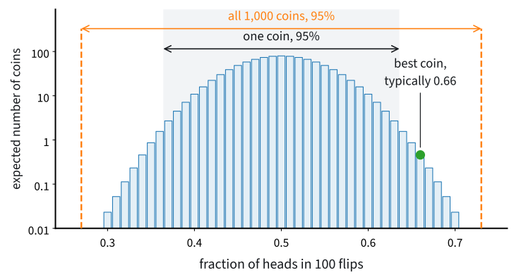
experiments in which the best coin leaves the one-coin band: 96%The best coin shows 66 heads in a typical experiment and between 64 and 69 in nine experiments out of ten. It leaves the single-coin band in about 96% of experiments, so a guarantee that is valid for every coin named in advance fails almost always for the coin chosen afterwards. No coin is biased. The selected coin is off by 16 points because we looked at 1,000 fluctuations and reported the largest.
Figure 27.8.1 shows why. Each coin leaves the band with probability \(0.0033\) on the upper side, a rare event, but among 1,000 coins about \(3.3\) are expected to do so. The tail that one coin almost never reaches is populated when a thousand coins are drawn.
The validation set of the opening differs from the coins in two ways, and neither matters for what follows. The configurations are scored on the same examples, so their scores are correlated, and their true errors differ. The bound below needs neither independence nor equal means.
What would cover the chosen function? If the largest deviation over the whole class,
\[ \sup_{f\in\mathcal F}\ \bigl|\hat R(f) - R(f)\bigr|, \]
is at most \(t\), then every function’s empirical risk is within \(t\) of its risk, including the one the learner picked. Bounds on this supremum are called uniform convergence bounds (Vapnik and Chervonenkis 1971). Choosing after seeing the data is safe if the guarantee was made for all candidates before seeing it, because the one we pick is one of them.
27.8.1.2 Finite Classes and the Union Bound
The simplest class is a finite list of candidates fixed in advance, such as a grid of hyperparameter configurations. For it, one fact from probability suffices: the probability that at least one of several events occurs is at most the sum of their probabilities. This is the union bound.
Proposition (finite-class uniform convergence). Let \(\mathcal F\) be a finite class fixed before the sample is drawn, let the loss take values in \([0,1]\), and let \(S\) be an i.i.d. sample of size \(n\). Then with probability at least \(1-\delta\),
\[ \bigl|\hat R(f) - R(f)\bigr| \le \sqrt{\frac{\log(2|\mathcal F|/\delta)}{2n}} \qquad\textrm{simultaneously for every } f\in\mathcal F . \tag{27.8.1}\]
Proof. For each fixed \(f\), Hoeffding gives \(P(|\hat R(f)-R(f)|\ge t)\le 2e^{-2nt^2}\). The union bound over the \(|\mathcal F|\) bad events bounds the probability that any of them occurs by \(2|\mathcal F|e^{-2nt^2}\). Setting this to \(\delta\) and solving for \(t\) gives the claim. \(\blacksquare\)
The only new step is the union bound; everything else is the single-function inequality. Compared with one function, the half-width has \(\log(2|\mathcal F|/\delta)\) in place of \(\log(2/\delta)\), so choosing among \(|\mathcal F|\) candidates adds \(\log|\mathcal F|\) under the square root.
On the coins, \(|\mathcal F|=1{,}000\) and \(n=100\) give the half-width \(\sqrt{\log(2{,}000/0.05)/200}=0.230\), so with probability at least 95% every coin, the best one included, shows between 27 and 73 heads. The typical best coin, at 66, is inside. The bound is conservative: the exact probability that some coin falls outside 27 to 73 heads is about 0.17%, against the 5% the bound allows. But it is valid, which the single-coin band was not.
At the scale of a validation set the logarithm keeps the extra data small. With \(n=10{,}000\) and \(\delta=0.05\), one function is certified to \(\pm0.0136\), 2,000 configurations to \(\pm0.0238\), and a million to \(\pm0.0296\). The million candidates widen the band by a factor of \(2.18\). Solving the bound for the sample size shows the dependence directly:
\[ n=\frac{\log(2/\delta)+\log|\mathcal F|}{2t^2}. \]
Each additional unit of \(\log|\mathcal F|\) adds \(1/(2t^2)\) examples. At a tolerance of \(t=0.01\), doubling the number of candidates adds \(\log 2/(2\cdot 10^{-4})\approx3{,}500\) validation examples.
The exponential tail of Hoeffding’s inequality is what makes the dependence logarithmic. Chebyshev’s inequality bounds the same deviation by \(\textrm{Var}(\hat R(f))/t^2\le 1/(4nt^2)\), because a \([0,1]\)-valued loss has variance at most \(\tfrac14\). The same union bound then gives \(|\mathcal F|/(4nt^2)=\delta\), that is,
\[ t=\sqrt{\frac{|\mathcal F|}{4n\delta}} . \]
For 2,000 configurations on 10,000 examples at \(\delta=0.05\) this is \(t=1\), which says nothing about a loss in \([0,1]\). Hoeffding gives \(t=0.024\) for the same pool. A polynomial tail makes the sample size grow like \(|\mathcal F|\), an exponential tail like \(\log|\mathcal F|\).
The proof uses one hypothesis in its first step, where Hoeffding is applied to each \(f\) separately: the class is fixed before the sample is drawn. A public leaderboard breaks this hypothesis. Each submission is chosen after seeing the scores of earlier ones on the same test set, so the submissions are not a fixed list and “for each fixed \(f\)” no longer applies. The guarantee then degrades much faster, as the analysis of adaptive data reuse shows (Dwork et al. 2015), and exercise 5 builds a submission that beats a random holdout without any knowledge of the task. The proposition thus turns the test-set-reuse warning of Section 3.6 into a number, and the leaderboard shows where that number stops applying.
27.8.2 Rademacher Complexity
The classes we train are infinite. Every weight vector \(\mathbf w\in\mathbb{R}^d\) defines a different linear classifier, and a union bound over infinitely many events gives nothing. The classical remedies either replace the class by finitely many representatives (covering numbers) or count the labelings it can produce on \(n\) points (the VC dimension, sketched in Section 3.6). The tool of this part is due to Koltchinskii and Panchenko and to Bartlett and Mendelson (2002) . It asks a question a practitioner can act on: how well can the class fit pure noise?
27.8.2.1 Correlation with Random Signs
If a class can fit labels that carry no information, it can also fit the noise in real labels, and then its empirical risks say little about its risks. To measure this we feed the class fictitious labels. Let \(\varepsilon_1,\ldots,\varepsilon_n\) be independent fair random signs, each \(+1\) or \(-1\) with probability \(\tfrac12\); they are called Rademacher variables. For a sign vector \(\boldsymbol\varepsilon\), the quantity \(\frac1n\sum_i\varepsilon_if(\mathbf x_i)\) is the correlation of \(f\) with the signs on the sample, and the best a class can do is its supremum over the class.
Definition. The empirical Rademacher complexity of a class \(\mathcal F\) of real-valued functions on the points \(S=(\mathbf x_1,\ldots,\mathbf x_n)\) is the expected best correlation the class achieves with random signs,
\[ \widehat{\mathfrak R}_S(\mathcal F) = \mathbb{E}_{\boldsymbol\varepsilon}\!\left[\, \sup_{f\in\mathcal F}\ \frac1n \sum_{i=1}^n \varepsilon_i\, f(\mathbf x_i) \right], \tag{27.8.2}\]
and its Rademacher complexity \(\mathfrak R_n(\mathcal F)=\mathbb{E}_S[\widehat{\mathfrak R}_S(\mathcal F)]\) is its average over samples of size \(n\).
A class that can match any sign pattern scores high; a class that cannot choose scores zero. The scale is set by the range of the functions. For a class with values in \([-1,1]\) each correlation is at most \(1\), and the value \(1\) is reached by the class of all functions into \([-1,1]\), which contains \(f(\mathbf x_i)=\varepsilon_i\) for every pattern (when the points are distinct). For a class with values in \([0,1]\) the largest possible value is \(\tfrac12\): the best choice is \(f(\mathbf x_i)=1\) exactly where \(\varepsilon_i=+1\), which scores the fraction of plus signs, \(\tfrac12\) on average. Below, predictors take values in \([-1,1]\) and losses in \([0,1]\).
The smallest case with something to choose is the class of the two constant functions \(\{+1,-1\}\). Its best correlation with a sign vector is \(\max(\bar\varepsilon,-\bar\varepsilon)=|\bar\varepsilon|\), where \(\bar\varepsilon\) is the average of the signs. For \(n=2\) the four patterns \((+,+),(+,-),(-,+),(-,-)\) give \(|\bar\varepsilon|=1,0,0,1\), so \(\widehat{\mathfrak R}_S=\tfrac12\). For \(n=4\) the sum of the signs is \(\pm4\) with probability \(\tfrac2{16}\), \(\pm2\) with probability \(\tfrac8{16}\) and \(0\) otherwise, which gives \(\widehat{\mathfrak R}_S=\tfrac38\). For large \(n\) the average \(\bar\varepsilon\) is approximately normal with variance \(1/n\), so \(\widehat{\mathfrak R}_S\approx\sqrt{2/(\pi n)}\); at \(n=100\) the exact value is \(0.0796\) against \(0.0798\). Even a class with only two members correlates with noise at the rate \(1/\sqrt n\), because the average of \(n\) signs has that spread. A class with one member has complexity \(0\): with nothing to choose, \(\mathbb{E}[\frac1n\sum_i\varepsilon_if(\mathbf x_i)]=0\).
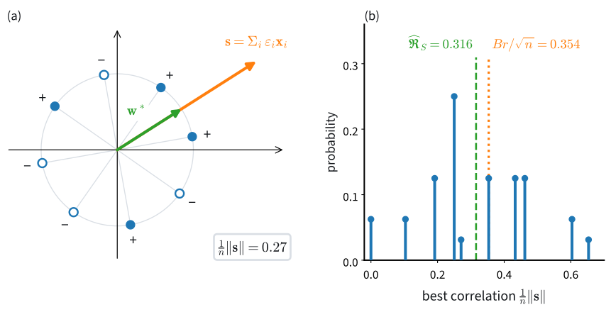
For a linear class the best correlation has a geometric meaning, which Figure 27.8.2 previews: it is the length of a signed sum of the inputs, divided by \(n\). Section 27.8.2.3 proves this.
Two more cases mark the ends of the scale. A finite class with values in \([-1,1]\) obeys Massart’s lemma, \(\widehat{\mathfrak R}_S(\mathcal F)\le\sqrt{2\log|\mathcal F|/n}\) (exercise 2), so its complexity grows only logarithmically with its size. The class of all functions into \([-1,1]\) reaches the maximum \(1\). Rademacher complexity therefore measures how freely the class can vary on the actual sample points, whatever the number of its parameters or members.
27.8.2.2 The Uniform Convergence Theorem
We now show that the Rademacher complexity bounds the largest deviation between empirical risk and risk. One distinction must be made first, because the predictions and the losses live in different classes. The predictor class \(\mathcal F\) contains the functions we fit. The functions whose averages we compare are the losses, so define the loss class
\[ \mathcal G=\bigl\{(\mathbf x,y)\mapsto\ell(f(\mathbf x),y):f\in\mathcal F\bigr\}, \]
with values in \([0,1]\). For \(g\in\mathcal G\) write \(z=(\mathbf x,y)\), \(R(g)=\mathbb{E}[g(z)]\) and \(\hat R_S(g)=\frac1n\sum_ig(z_i)\). The risk of a predictor is the risk of its loss.
Proposition (uniform convergence via Rademacher complexity) (Bartlett and Mendelson 2002). Let \(S=(z_1,\ldots,z_n)\) be an i.i.d. sample and let \(\mathcal G\) be a class of functions with values in \([0,1]\). Then with probability at least \(1-\delta\),
\[ R(g) \le \hat R_S(g) + 2\,\mathfrak R_n(\mathcal G) + \sqrt{\frac{\log(1/\delta)}{2n}} \qquad\textrm{simultaneously for every } g\in\mathcal G . \tag{27.8.3}\]
The bound has the shape of the finite-class one: an empirical risk, a term for the richness of the class, and a confidence term that would be there for a single function. The richness term is twice the class’s ability to fit random signs.
Proof. We show \(\mathbb{E}_S\bigl[\sup_g(R(g)-\hat R_S(g))\bigr]\le2\mathfrak R_n(\mathcal G)\) in three steps; the high-probability form follows afterwards.
I. Ghost sample. Let \(S'=(z'_1,\ldots,z'_n)\) be an independent copy of \(S\), used only inside the proof. Since \(R(g)=\mathbb{E}_{S'}[\hat R_{S'}(g)]\), and a supremum of expectations is at most the expectation of the supremum,
\[ \mathbb{E}_S\Bigl[\sup_{g\in\mathcal G}\bigl(R(g)-\hat R_S(g)\bigr)\Bigr] \le \mathbb{E}_{S,S'}\Bigl[\sup_{g\in\mathcal G}\ \frac1n\sum_{i=1}^n \bigl(g(z'_i)-g(z_i)\bigr)\Bigr]. \tag{27.8.4}\]
The unknown risk has been replaced by a second sample.
- Sign swap. Exchanging \(z_i\) with \(z'_i\) leaves the joint distribution of \((S,S')\) unchanged, because the two points are independent draws from the same distribution. The exchange flips the sign of the \(i\)-th difference \(g(z'_i)-g(z_i)\) for every \(g\) at once. So for any fixed signs \(\varepsilon_1,\ldots,\varepsilon_n\) the right-hand side of Equation 27.8.4 does not change if the \(i\)-th difference is multiplied by \(\varepsilon_i\). Nor does it change when the signs are drawn at random:
\[ \mathbb{E}_{S,S'}\Bigl[\sup_{g}\ \frac1n\sum_i\bigl(g(z'_i)-g(z_i)\bigr)\Bigr] = \mathbb{E}_{S,S',\boldsymbol\varepsilon}\Bigl[\sup_{g}\ \frac1n\sum_i \varepsilon_i\bigl(g(z'_i)-g(z_i)\bigr)\Bigr]. \]
- Split. The supremum of a sum is at most the sum of the suprema, so the right-hand side is at most
\[ \mathbb{E}_{S',\boldsymbol\varepsilon}\Bigl[\sup_{g}\ \frac1n\sum_i \varepsilon_i\,g(z'_i)\Bigr] + \mathbb{E}_{S,\boldsymbol\varepsilon}\Bigl[\sup_{g}\ \frac1n\sum_i (-\varepsilon_i)\,g(z_i)\Bigr] = 2\,\mathfrak R_n(\mathcal G), \]
because \(-\boldsymbol\varepsilon\) has the same distribution as \(\boldsymbol\varepsilon\), so each term is \(\mathfrak R_n(\mathcal G)\). The split produces the factor \(2\).
For the high-probability form, consider \(\Phi(S)=\sup_g(R(g)-\hat R_S(g))\). Changing one sample point changes each \(\hat R_S(g)\) by at most \(1/n\), and therefore changes \(\Phi\) by at most \(1/n\). McDiarmid’s inequality (McDiarmid 1989), the extension of Hoeffding’s inequality from sums to functions that no single input can move much, then gives \(P(\Phi-\mathbb{E}\Phi\ge t)\le e^{-2nt^2}\) (exercise 1). Setting the right-hand side to \(\delta\) and combining with the bound on \(\mathbb{E}\Phi\) gives Equation 27.8.3. \(\blacksquare\)
The intuition is that the ghost sample stands in for the population. Swapping a real point with its ghost changes nothing, because the two are exchangeable, and after the swaps only coin flips remain: the deviation of the class from the truth is controlled by how well it can follow random signs.
The theorem can be checked at its ends. For a class with one member, \(\mathfrak R_n=0\) and Equation 27.8.3 is one-sided Hoeffding. For a finite class, Massart’s lemma turns it into Equation 27.8.1 with larger constants: for 2,000 configurations on 10,000 examples the complexity term alone is \(2\sqrt{2\log 2000/n}=0.078\), against the union bound’s whole half-width of \(0.024\). The Rademacher route is weaker for finite classes, but it also applies to infinite ones. For classes of binary classifiers, counting the labelings the class can realize on \(n\) points gives \(\mathfrak R_n\lesssim\sqrt{d_{\mathrm{VC}}\log n/n}\) (Boucheron et al. 2005). Here \(d_{\mathrm{VC}}\) is the VC dimension, the largest number of points on which the class realizes every labeling.
At the other end, a loss class with values in \([0,1]\) has \(\mathfrak R_n(\mathcal G)\le\tfrac12\). When equality holds, the complexity term is \(1\) and the bound says nothing. For classifiers with the 0-1 loss, the two complexities stand in a fixed ratio. Let the predictors take values in \(\{-1,+1\}\) and use the 0-1 loss, \(g(\mathbf x,y)=(1-yf(\mathbf x))/2\). Then \(\sum_i\varepsilon_ig(z_i)=\tfrac12\sum_i\varepsilon_i+\tfrac12\sum_i(-\varepsilon_iy_i)f(\mathbf x_i)\). The first sum has mean zero and does not depend on \(f\), and for fixed labels \(-\varepsilon_iy_i\) is again a fair random sign, so
\[ \widehat{\mathfrak R}_S(\mathcal G)=\tfrac12\,\widehat{\mathfrak R}_S(\mathcal F). \]
A predictor class that fits every sign pattern on the sample has \(\widehat{\mathfrak R}_S(\mathcal F)=1\), so twice the loss complexity is \(1\) and the theorem guarantees nothing for it.
27.8.2.3 The Linear Class
The theorem is useful only if the complexity can be computed for a class we care about. For linear functions with a bounded weight norm the computation takes four lines, and its answer does not involve the dimension.
Proposition (Rademacher complexity of a norm-bounded linear class). Let \(\mathcal F=\{\mathbf x\mapsto\langle\mathbf w,\mathbf x\rangle : \|\mathbf w\|_2\le B\}\) and suppose the sample satisfies \(\|\mathbf x_i\|_2\le r\) for all \(i\). Then
\[ \widehat{\mathfrak R}_S(\mathcal F) = \frac Bn\,\mathbb{E}_{\boldsymbol\varepsilon}\Bigl\|\sum_{i=1}^n\varepsilon_i\mathbf x_i\Bigr\| \le \frac{B\,r}{\sqrt n}. \tag{27.8.5}\]
Proof. The supremum is explicit. By linearity and Cauchy–Schwarz, with equality at \(\mathbf w\) of length \(B\) aligned with the signed sum,
\[ \sup_{\|\mathbf w\|\le B}\ \frac1n\sum_{i=1}^n \varepsilon_i \langle\mathbf w,\mathbf x_i\rangle = \sup_{\|\mathbf w\|\le B}\ \frac1n \Bigl\langle\mathbf w,\ \sum_i \varepsilon_i\mathbf x_i\Bigr\rangle = \frac Bn\,\Bigl\|\sum_{i=1}^n \varepsilon_i\mathbf x_i\Bigr\| . \]
Taking the expectation gives the equality in the proposition. For the bound, the square root is concave, so \(\mathbb{E}\|\cdot\|\le\sqrt{\mathbb{E}\|\cdot\|^2}\), and expanding the square,
\[ \mathbb{E}_{\boldsymbol\varepsilon}\Bigl\|\sum_i\varepsilon_i\mathbf x_i\Bigr\| \le \sqrt{\sum_{i,j} \mathbb{E}[\varepsilon_i\varepsilon_j]\, \langle\mathbf x_i,\mathbf x_j\rangle} = \sqrt{\sum_i \|\mathbf x_i\|^2} \le r\sqrt n . \]
The cross terms vanish because independent signs have \(\mathbb{E}[\varepsilon_i\varepsilon_j]=0\) for \(i\ne j\). Multiplying by \(B/n\) gives \(Br/\sqrt n\). \(\blacksquare\)
Panel (a) of Figure 27.8.2 draws the first step of this proof: the best weight vector points along the signed sum.
Only one step of the proof loses anything. The identity \(\mathbb{E}\|\sum_i\varepsilon_i\mathbf x_i\|^2=\sum_i\|\mathbf x_i\|^2\) is exact, so the slack is all in the step from the mean length of the signed sum to its root-mean-square length. That step is tight when the length varies little from one sign pattern to the next. For the eight points of the figure the slack is 11% (\(0.316\) against \(0.354\)). In the plane, a signed sum of many unit vectors in spread-out directions is approximately a two-dimensional Gaussian vector, whose length has mean \(\sqrt\pi/2\approx0.89\) times its root-mean-square, so the slack stays near 11% however many points there are. In twenty dimensions the length of the signed sum concentrates, by the thin shell of Section 27.7.2.1, and the slack falls to about 1%.
The dimension \(d\) does not appear in Equation 27.8.5. Two linear classes have the same bound whenever the product \(Br\) is the same, whether they act on ten features or on a million; the dimension matters only through its effect on \(B\) and \(r\). In this bound the capacity of a linear model is set by the product of its weight norm and its input radius, not by its number of parameters. Weight decay (Section 2.7) keeps \(\|\mathbf w\|\) small, and so keeps the class that contains the fitted model small.
A reader may object that the proposition needs \(B\) fixed before the data, while the norm of a trained weight vector is known only afterwards. The objection is right, and a union bound over radii answers it. Apply the bound to each radius \(B_j=2^j\) with failure probability \(\delta_j=\delta/(j(j+1))\), which sum to \(\delta\), and use the smallest radius that contains the fitted vector. For \(\|\mathbf w\|>1\) this loses at most a factor \(2\) in the complexity term and adds a term of order \(\sqrt{\log\log\|\mathbf w\|/n}\) (exercise 3).
The theorem needs the complexity of the loss class, and the proposition computes that of the predictor class. A Lipschitz loss connects them.
Lemma (contraction) (Boucheron et al. 2013). Let \(\phi_1,\ldots,\phi_n:\mathbb{R}\to\mathbb{R}\) each be \(L\)-Lipschitz. Then for any class \(\mathcal F\) and points \(\mathbf x_1,\ldots,\mathbf x_n\),
\[ \mathbb{E}_{\boldsymbol\varepsilon}\Bigl[\sup_{f\in\mathcal F}\sum_{i=1}^n \varepsilon_i\,\phi_i\bigl(f(\mathbf x_i)\bigr)\Bigr] \le L\,\mathbb{E}_{\boldsymbol\varepsilon}\Bigl[\sup_{f\in\mathcal F} \sum_{i=1}^n\varepsilon_i\,f(\mathbf x_i)\Bigr]. \tag{27.8.6}\]
Composing with a function that stretches distances by at most \(L\) multiplies the complexity by at most \(L\). Each \(\phi_i\) may differ, which is what a loss needs: at the point \(i\) the loss is the function \(u\mapsto\ell(u,y_i)\) of the prediction, with the label \(y_i\) fixed. No centering is required, since adding a constant \(c\) to \(\phi_i\) adds \(c\,\varepsilon_i\), whose expectation is zero. We state the lemma without proof.
The theorem also needs losses in \([0,1]\). The hinge and logistic losses are not bounded by \(1\): on the class they reach about \(1+Br\), so they must be divided by that maximum before the theorem applies. A loss that is bounded from the start is the ramp loss on the margin \(u=yf(\mathbf x)\),
\[ \phi_\gamma(u)=\min\bigl\{1,\max\{0,\,1-u/\gamma\}\bigr\}, \]
which is \(1\) for a mistake, \(0\) for a correct prediction with margin at least \(\gamma\), and linear in between. It lies above the 0-1 loss and is \((1/\gamma)\)-Lipschitz.
Write \(\hat R_\gamma(\mathbf w)\) for the average of the ramp loss \(\frac1n\sum_i\phi_\gamma(y_i\langle\mathbf w,\mathbf x_i\rangle)\) on the sample. With \(\|\mathbf x\|\le r\) for every input, the contraction lemma and the linear-class proposition give a loss-class complexity of at most \(Br/(\gamma\sqrt n)\), and the theorem gives, with probability at least \(1-\delta\), for every \(\mathbf w\) with \(\|\mathbf w\|\le B\),
\[ P\bigl(y\langle\mathbf w,\mathbf x\rangle\le0\bigr) \le \hat R_\gamma(\mathbf w) + \frac{2Br}{\gamma\sqrt n} + \sqrt{\frac{\log(1/\delta)}{2n}} . \tag{27.8.7}\]
The left side is the true error rate of the linear classifier; the right side is its training ramp loss plus two terms we can evaluate. For \(Br/\gamma=10\), \(n=50{,}000\) and \(\delta=0.05\), the complexity term is \(0.089\) and the confidence term \(0.005\), together \(0.095\). With \(B=10\gamma/r\) fixed in advance, a linear classifier in the class that separates its training data with margin \(\gamma\) has, with probability at least 95%, a true error below \(9.5\%\). Fitting random labels with a margin forces \(Br/\gamma\) up. Once it passes about \(10.6\) the two terms exceed \(0.1\), and near \(Br/\gamma\approx110\) the complexity term alone reaches \(1\).
27.8.2.4 Rademacher Complexity in Numbers
The proposition gives the complexity of the linear class as an expected length, and the expectation can be estimated by averaging over random sign vectors. The cell below does this for 50 unit-norm points in \(d=2\), \(20\) and \(1{,}000\) dimensions, and compares with the bound \(Br/\sqrt n=1/\sqrt{50}\).
n, B, num_signs = 50, 1.0, 2000
signs = rng.choice([-1.0, 1.0], size=(num_signs, n))  # rows: sign vectors
for d in (2, 20, 1000):
    X = rng.standard_normal((n, d))
    X /= np.linalg.norm(X, axis=1, keepdims=True)       # ||x_i|| = r = 1
    sup_corr = B * np.linalg.norm(signs @ X, axis=1) / n  # closed-form sup
    print(f'd = {d:4d}: Monte-Carlo R_S = {sup_corr.mean():.3f}, '
f'bound B r / sqrt(n) = {B / np.sqrt(n):.3f}')d = 2: Monte-Carlo R_S = 0.124, bound B r / sqrt(n) = 0.141
d = 20: Monte-Carlo R_S = 0.140, bound B r / sqrt(n) = 0.141
d = 1000: Monte-Carlo R_S = 0.141, bound B r / sqrt(n) = 0.141d = 2: Monte-Carlo R_S = 0.125, bound B r / sqrt(n) = 0.141
d = 20: Monte-Carlo R_S = 0.140, bound B r / sqrt(n) = 0.141
d = 1000: Monte-Carlo R_S = 0.141, bound B r / sqrt(n) = 0.141d = 2: Monte-Carlo R_S = 0.129, bound B r / sqrt(n) = 0.141
d = 20: Monte-Carlo R_S = 0.140, bound B r / sqrt(n) = 0.141
d = 1000: Monte-Carlo R_S = 0.141, bound B r / sqrt(n) = 0.141d = 2: Monte-Carlo R_S = 0.125, bound B r / sqrt(n) = 0.141
d = 20: Monte-Carlo R_S = 0.140, bound B r / sqrt(n) = 0.141
d = 1000: Monte-Carlo R_S = 0.141, bound B r / sqrt(n) = 0.141The estimate is about \(0.125\) in the plane and \(0.139\) to \(0.141\) in 20 and 1,000 dimensions, against the bound \(0.141\). The value in the plane is the Gaussian prediction \(0.89\times0.141=0.125\), and in higher dimensions the bound is nearly exact. Going from 20 to 1,000 dimensions leaves the complexity unchanged. A unit-norm linear class on fifty unit-norm points reaches an average correlation of about \(0.14\) with pure noise, and in 2 and 20 dimensions single sign draws reach above \(0.2\).
The other end of the scale is a class rich enough to interpolate, that is, to reproduce any labels exactly on the sample. Least squares on \(p=2n\) Gaussian features, fit with the pseudoinverse of Section 24.4.3.1, returns for every sign vector the interpolant \(\mathbf w=\boldsymbol\Phi^+\boldsymbol\varepsilon\) of smallest norm, where \(\boldsymbol\Phi\in\mathbb{R}^{n\times p}\) holds the features of the points as rows. Its correlation with the signs is \(1\) for every pattern, by construction. The informative number is the norm the fits need. Since \(\mathbf w=\boldsymbol\Phi^\top(\boldsymbol\Phi\boldsymbol\Phi^\top)^{-1}\boldsymbol\varepsilon\),
\[ \|\mathbf w\|^2=\boldsymbol\varepsilon^\top(\boldsymbol\Phi\boldsymbol\Phi^\top)^{-1}\boldsymbol\varepsilon, \qquad \mathbb{E}\|\mathbf w\|^2=\operatorname{tr}\,\mathbb{E}\bigl[(\boldsymbol\Phi\boldsymbol\Phi^\top)^{-1}\bigr]=\frac{n}{p-n-1}, \]
where the last step uses the mean of an inverse Wishart matrix, \(\mathbb{E}[(\boldsymbol\Phi\boldsymbol\Phi^\top)^{-1}]=\mathbf I_n/(p-n-1)\) for standard Gaussian entries and \(p>n+1\) (exercise 4). For \(n=50\) and \(p=100\) the prediction is \(\|\mathbf w\|\approx\sqrt{50/49}=1.01\). The cell measures the norms and the bound \(Br/\sqrt n\) of the smallest ball that contains all 2,000 fits.
p = 2 * n                                     # more features than points
Phi = rng.standard_normal((n, p))
W = np.linalg.pinv(Phi) @ signs.T             # min-norm fit of each sign vector
w_norm = np.linalg.norm(W, axis=0)
r = np.linalg.norm(Phi, axis=1).max()         # input radius: largest row norm
print(f'mean ||w|| = {w_norm.mean():.2f} (predicted '
      f'{np.sqrt(n / (p - n - 1)):.2f}), largest {w_norm.max():.2f}')
print(f'r = {r:.1f}, B r / sqrt(n) with B = largest ||w||: '
f'{w_norm.max() * r / np.sqrt(n):.1f}')mean ||w|| = 0.98 (predicted 1.01), largest 1.39
r = 11.8, B r / sqrt(n) with B = largest ||w||: 2.3mean ||w|| = 1.03 (predicted 1.01), largest 1.47
r = 11.2, B r / sqrt(n) with B = largest ||w||: 2.3mean ||w|| = 1.01 (predicted 1.01), largest 1.45
r = 11.5, B r / sqrt(n) with B = largest ||w||: 2.4mean ||w|| = 0.99 (predicted 1.01), largest 1.42
r = 11.5, B r / sqrt(n) with B = largest ||w||: 2.3The mean norm matches the prediction, \(1.0\) against \(1.01\). The rows of \(\boldsymbol\Phi\) have length about \(\sqrt p=10\), the longest about 11 to 12.5, and the ball that holds the 2,000 fits gives \(Br/\sqrt n\) between about 2 and 2.8. A ball that holds an interpolant of every one of the \(2^{50}\) sign vectors is at least as large, and for that ball the value must be at least \(1\). The class then fits every sign pattern, so its \(\widehat{\mathfrak R}_S\) is at least \(1\), and the proposition bounds \(\widehat{\mathfrak R}_S\) by \(Br/\sqrt n\).
The same arithmetic applies to networks. In Section 4.5.1.1 an MLP was trained to zero error on random labels of its training images, as Zhang et al. (2021) did for image classifiers. The class “this architecture, trained this way” therefore fits every sign pattern on those inputs, and its Rademacher complexity there is about \(1\). Twice the complexity of the loss class is then also about \(1\), and Equation 27.8.3 certifies nothing. Yet the same network generalizes on real labels. What decides its test error is therefore invisible to a bound over the whole class: the data, the optimizer, and the solution it reached. The next part examines a model in which the solution can be computed in closed form. There, the solution’s norm and the conditioning of the fit explain a test curve that the class bound cannot.
27.8.3 Interpolation and Double Descent
In Section 2.6, the test error of polynomial fits followed a U: it fell as the degree grew, then rose sharply as the fit approached an exact match of the training points. Section 4.5.2 continued past that point with a network whose hidden layer stayed frozen at its random initialization. The test error peaked at the width \(h=n\) at which an exact fit first became possible and fell again beyond it, and the smallest singular value of the hidden representation was tiny at the peak. Here we repeat the construction on synthetic data, where every quantity in the mechanism can be computed. The features are \(\boldsymbol\phi(\mathbf x)=\mathrm{ReLU}(\mathbf V\mathbf x)\) with a frozen random matrix \(\mathbf V\), a random-features model (Rahimi and Recht 2007), and only the linear head \(\mathbf w\) is fit.
27.8.3.1 The Minimum-Norm Interpolant
To see why the threshold is special we need the solution in closed form. With \(p\) features and \(n\) points, the feature matrix \(\boldsymbol\Phi\in\mathbb{R}^{n\times p}\) has the feature vectors of the training points as rows, and we fit \(\mathbf w=\boldsymbol\Phi^+\mathbf y\). Below \(p=n\) least squares cannot match all \(n\) labels and returns the best compromise. At \(p=n\) it must invert a square matrix. Above \(p=n\) infinitely many weight vectors fit exactly, and the pseudoinverse returns the one of smallest norm.
The singular value decomposition shows all three cases at once. Let \(\boldsymbol\Phi\) have full rank \(q=\min(n,p)\) and singular value decomposition \(\boldsymbol\Phi=\sum_{i=1}^q\sigma_i\mathbf u_i\mathbf v_i^\top\), with \(\sigma_1\ge\cdots\ge\sigma_q>0\). Then
\[ \mathbf w=\boldsymbol\Phi^+\mathbf y=\sum_{i=1}^{q} \frac{\langle\mathbf u_i,\mathbf y\rangle}{\sigma_i}\,\mathbf v_i . \tag{27.8.8}\]
Every component of \(\mathbf y\) along a left singular vector is divided by its singular value, so the smallest singular value \(\sigma_{\min}=\sigma_q\) amplifies most. Whatever part of \(\mathbf y\) lies along \(\mathbf u_q\) enters the solution with the factor \(1/\sigma_{\min}\). This holds for label noise and equally for the part of the target that the features represent badly.
For \(p<n\) the fit \(\boldsymbol\Phi\mathbf w\) is the projection of \(\mathbf y\) onto the \(p\) directions \(\mathbf u_i\), and the rest of \(\mathbf y\) is left as residual. At \(p=n\) there are \(n\) directions, the fit is exact, and nothing is left over to absorb the badly represented part. A random square ReLU-feature matrix is invertible with overwhelming probability, but almost never well invertible: its smallest singular value is small, and the condition-number analysis of Section 24.4.3.2 says that the solution then moves far in the direction \(\mathbf v_q\). Adding features beyond \(n\) gives the matrix more room, and its smallest singular value grows again.
Past the threshold the norm of the solution can only fall as features are added, provided the features are nested: the model with \(p+1\) features uses the first \(p\) features of the model with \(p\), plus one more.
Proposition (nesting). For nested features and \(p\ge n\), with \(\boldsymbol\Phi_p\) of full row rank, the minimum-norm interpolants satisfy \(\|\mathbf w^{(p+1)}_{\min}\|\le\|\mathbf w^{(p)}_{\min}\|\).
Proof. Padding \(\mathbf w^{(p)}_{\min}\) with a zero weight for the new feature gives an interpolant with \(p+1\) features of the same norm. The minimum-norm interpolant with \(p+1\) features is no longer than any interpolant, in particular this one. \(\blacksquare\)
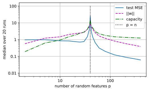
The argument needs exact interpolation. Below \(p=n\) the least-squares solution is not an interpolant, and its norm grows with \(p\): in the sweep below it rises from about \(0.5\) at \(p=2\) to about \(2\) at \(p=15\).
The linear-class bound suggests what to track along the sweep. Its capacity term for the class that contains the fitted head is the product \(\|\mathbf w\|\cdot\max_i\|\boldsymbol\phi(\mathbf x_i)\|/\sqrt n\): the norm of the solution times the radius of the features, divided by \(\sqrt n\). The feature radius grows like \(\sqrt p\) as features are added, while the norm of the solution falls past the threshold, so the product could go either way. We measure it.
27.8.3.2 A Double-Descent Sweep
We now compute the whole curve. The data are forty training points from a linear teacher \(y=\langle\boldsymbol\beta,\mathbf x\rangle\) in fifteen dimensions, with \(\|\boldsymbol\beta\|=1\) and label noise of standard deviation \(0.1\). The features are ReLU random features with nested columns, and the head is fit by pinv: least squares below the threshold, the minimum-norm interpolant above it. We sweep \(p\) from \(2\) to \(400\) through \(p=n=40\), with the neighbours \(p=39\) and \(41\) included so that the peak is resolved. For every fit we record the test error, the training error, \(\|\mathbf w\|\), \(\sigma_{\min}\) and the capacity product. We also record the two parts of the test error that Section 27.8.3.3 separates: the clean part, the error of the same fit made to noise-free labels, and the noise part, the extra error that the label noise adds. Medians over 20 independent runs keep the curve readable.
n, n_test, d_in, p_max, trials, noise = 40, 500, 15, 400, 20, 0.1
p_grid = np.array([2, 5, 10, 15, 20, 25, 30, 35, 38, 39, 40, 41, 42, 45, 50,
                   60, 80, 120, 200, 400])
keys = ('test', 'train', 'norm', 's_min', 'capacity', 'clean', 'noise')
stats = np.zeros((len(keys), trials, len(p_grid)))
for tr in range(trials):
    beta = rng.standard_normal(d_in)
    beta /= np.linalg.norm(beta)                     # teacher: y = <beta, x>
    X, X_te = (rng.standard_normal((size, d_in)) for size in (n, n_test))
    y_clean, y_te = X @ beta, X_te @ beta
    y = y_clean + noise * rng.standard_normal(n)     # noisy training labels
    V = rng.standard_normal((p_max, d_in)) / np.sqrt(d_in)
    Phi, Phi_te = np.maximum(X @ V.T, 0), np.maximum(X_te @ V.T, 0)
    for j, p in enumerate(p_grid):                   # nested feature prefixes
        F, F_te = Phi[:, :p], Phi_te[:, :p]
        P = np.linalg.pinv(F)                        # least squares / min norm
        w = P @ y
        r = np.linalg.norm(F, axis=1).max()          # feature radius
        stats[:, tr, j] = (
            np.mean((F_te @ w - y_te) ** 2),                 # test MSE
            np.mean((F @ w - y) ** 2),                       # training MSE
            np.linalg.norm(w),                               # ||w||
            np.linalg.svd(F, compute_uv=False).min(),        # sigma_min
            np.linalg.norm(w) * r / np.sqrt(n),              # capacity
            np.mean((F_te @ (P @ y_clean) - y_te) ** 2),     # clean part
            noise ** 2 * np.linalg.norm(F_te @ P) ** 2 / n_test)  # noise part
med = dict(zip(keys, np.median(stats, axis=1)))
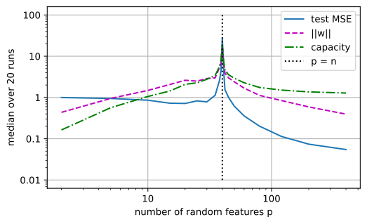
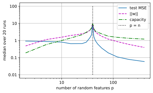
The plot shows the medians of the test error, the solution norm, and the capacity product against \(p\) on logarithmic axes, with the threshold \(p=n\) marked.
d2l.plot([p_grid] * 3 + [[n, n]],
         [med['test'], med['norm'], med['capacity'], [1e-2, 1e2]],
         'number of random features p', 'median over 20 runs',
         legend=['test MSE', '||w||', 'capacity', 'p = n'], xscale='log',
         yscale='log', fmts=('-', 'm--', 'g-.', 'k:'), figsize=(6, 3.5))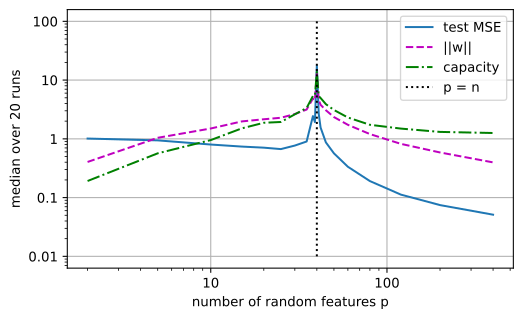
The table lists the medians at seven feature counts: below the threshold, at it, and above it.
print('   p ' + ' '.join(f'{key:>8}' for key in keys))
for p in (15, 38, 40, 42, 50, 80, 400):
    row = [med[key][p_grid == p][0] for key in keys]
print(f'{p:4d} ' + ' '.join(f'{v:8.2g}' for v in row)) p test train norm s_min capacity clean noise
15 0.74 0.26 2 0.89 1.5 0.73 0.0071
38 2.4 0.0028 4.9 0.08 5.4 1.7 0.25
40 18 4.6e-29 13 0.02 14 8.3 3.3
42 1.6 1.4e-29 3.8 0.095 5 1.4 0.21
50 0.57 1.2e-29 2.3 0.24 3.1 0.47 0.062
80 0.19 9.6e-30 1.2 0.7 1.7 0.16 0.021
400 0.051 5.2e-30 0.4 2.7 1.3 0.045 0.0093 p test train norm s_min capacity clean noise
15 0.73 0.29 2.1 0.89 1.4 0.7 0.0069
38 2.6 0.005 5.4 0.099 5.7 2.3 0.19
40 28 7e-29 18 0.019 19 23 3.4
42 1.6 1.1e-29 3.9 0.099 4.6 1.8 0.19
50 0.61 1.6e-29 2.4 0.27 2.9 0.6 0.059
80 0.2 1.6e-29 1.1 0.73 1.7 0.17 0.021
400 0.055 8.1e-30 0.4 2.8 1.3 0.044 0.0096 p test train norm s_min capacity clean noise
15 0.83 0.28 2 0.99 1.5 0.81 0.0067
38 3.6 0.0068 5.6 0.086 6.8 3.5 0.26
40 25 9.9e-29 14 0.023 16 23 2.2
42 3 2.9e-29 5.5 0.076 6.3 3.4 0.34
50 0.66 1.8e-29 2.6 0.25 3.1 0.65 0.063
80 0.2 1e-29 1.2 0.75 1.8 0.19 0.02
400 0.062 1.5e-29 0.39 2.8 1.2 0.056 0.0087 p test train norm s_min capacity clean noise
15 0.65 0.25 2 0.98 1.4 0.65 0.0067
38 2.1 0.0042 5.1 0.066 5.5 3 0.3
40 9.1 4.3e-29 9.1 0.023 9.4 10 2
42 1.7 1.3e-29 4.2 0.075 5 1.9 0.23
50 0.62 1.2e-29 2.4 0.25 3 0.58 0.056
80 0.19 1.1e-29 1.2 0.75 1.8 0.16 0.021
400 0.059 8.9e-30 0.39 2.7 1.2 0.053 0.0093Below the threshold the test error first falls, from about \(1\) at \(p=2\) to a minimum of roughly \(0.6\) to \(0.8\) somewhere between \(p=15\) and \(p=30\), then rises, as the U-curve leads us to expect. At \(p=40=n\) the training error drops from a few times \(10^{-3}\) at \(p=38\) to about \(10^{-28}\), which is exact interpolation up to floating point. At the same point the test error peaks, typically one to two orders of magnitude above the underparameterized minimum. The median over 20 trials lands anywhere between about 5 and 50 from one run of the cell to the next, because the peak is heavy-tailed: for a square Gaussian matrix \(\mathbb{E}[1/\sigma_{\min}^2]\) is infinite. The solution norm jumps to between about 6 and 20, and \(\sigma_{\min}\) falls to about \(0.01\) to \(0.04\), against \(0.05\) to \(0.12\) at \(p=38\) and about \(2.8\) at \(p=400\).
Past the threshold the norm falls steadily, as the nesting proposition requires (it does so in every trial, not only in the medians), down to about \(0.4\) at \(p=400\). The test error follows: between about \(0.5\) and \(0.9\) at \(p=50\), \(0.2\) at \(p=80\), about \(0.12\) at \(p=120\), and \(0.04\) to \(0.07\) at \(p=400\), roughly ten times below the best underparameterized model. The training error is zero up to floating point everywhere past the threshold, so no criterion based on the training error can tell \(p=42\) from \(p=400\). The norm, the smallest singular value and the capacity product all can. The best model in the experiment is the most overparameterized one, fitting noisy data exactly, with ten times more parameters than data points.
The capacity product peaks at the threshold with values of about 8 to 25, falls past it, and reaches about \(1.2\) to \(1.3\) at \(p=400\). It follows the shape of the test curve, but it certifies nothing, for two reasons. First, past the threshold it stays above \(1\). A complexity bound of \(1\) or more allows the class to fit every sign pattern, so the resulting bound on the test error is empty. Second, its \(B\) was read off the fit rather than fixed in advance.
The peak is not caused by the label noise. Rerunning the sweep with noise = 0 leaves a peak of the same size, and the table shows why. At \(p=40\) the clean part of the test error is larger than the noise part, usually several times larger. The linear teacher is not a combination of finitely many ReLU features, and the part of the target that the features represent badly is what \(\sigma_{\min}\) divides. With a target that is an exact combination of the first ten features and no noise, there is no peak at all (exercise 8).
27.8.3.3 Benign Overfitting
One puzzle remains. The \(p=400\) model reproduces every noisy training label exactly, yet it tests best. Why does fitting the noise cost so little there?
The test error separates into two parts we can compute. Write the training labels as \(\mathbf y=\mathbf y_0+\boldsymbol\xi\), with \(\mathbf y_0\) the noise-free labels and \(\boldsymbol\xi\) independent noise of variance \(\sigma_\xi^2=0.01\) per label. Then \(\mathbf w=\boldsymbol\Phi^+\mathbf y_0+\boldsymbol\Phi^+\boldsymbol\xi\), and the predictions at the test points are \(\boldsymbol\Phi_{\mathrm{te}}\boldsymbol\Phi^+\mathbf y_0+\boldsymbol\Phi_{\mathrm{te}}\boldsymbol\Phi^+\boldsymbol\xi\). In the squared test error, the cross term between these two parts has mean zero because \(\boldsymbol\xi\) does. Averaged over the noise, the test error over \(n_{\mathrm{te}}\) test points is
\[ \mathbb{E}_{\boldsymbol\xi}\bigl[\textrm{test error}\bigr] = \underbrace{\frac{1}{n_{\mathrm{te}}}\bigl\|\boldsymbol\Phi_{\mathrm{te}}\boldsymbol\Phi^+\mathbf y_0-\mathbf y_{\mathrm{te}}\bigr\|^2}_{\textrm{clean part}} + \underbrace{\frac{\sigma_\xi^2}{n_{\mathrm{te}}}\bigl\|\boldsymbol\Phi_{\mathrm{te}}\boldsymbol\Phi^+\bigr\|_F^2}_{\textrm{noise part}} . \]
The clean part is the error the same procedure would make with noise-free labels; the noise part is what the noise adds. The last two columns of the table print them. At \(p=40\) the noise part is about \(1\) to \(4\), a hundred times or more the noise variance \(0.01\), and the clean part is larger still. At \(p=42\) the noise part is a few tenths, at \(p=80\) about \(0.02\), and at \(p=400\) just under \(0.01\). Far past the threshold, interpolating the noise adds about the noise variance itself to the test error.
The clean part falls from about 5 to 40 at the peak to about \(0.04\) to \(0.06\) at \(p=400\). Most of the gain past the threshold therefore comes from a better approximation of the target.
Equation 27.8.8 explains why the noise costs so little. The signal is carried by the few directions with large \(\sigma_i\). Minimizing the norm spreads the interpolated noise across the many directions with small \(\sigma_i\), and each of them changes the predictions at new points only slightly. Overfitting is benign when the spectrum has this shape: a few strong directions to carry the signal, and many weak ones to absorb the noise.
Bartlett et al. (2020) make this precise for linear regression, through two effective ranks of the covariance of the inputs, and exercise 9 measures them. In deep networks the features are learned and change the spectrum during training, and a theory that predicts a given network’s test error from first principles is still open.
We can now say how much more data a choice among a fixed list of candidates requires: a \(\log|\mathcal F|\) under the square root. We can compute the Rademacher complexity of a norm-bounded linear class and turn it into a margin bound with numbers. We can also read a double-descent curve as a conditioning event at the threshold, followed by a shrinking minimum-norm solution. Every bound in this section covers the worst function in a class fixed before the data, while the function we use is the one an algorithm reached, and the sweep shows that this function can be excellent while the class bound stays above \(1\). A guarantee that depends on the algorithm and the data, rather than on the class alone, is the open question this section leaves.
27.8.4 Summary
A guarantee for one function fixed before the data says nothing about the function chosen because it looked best on the data. The best of 1,000 fair coins shows about 66 heads in 100 flips, outside the band that holds for each coin named in advance. Uniform convergence repairs this by asking for a guarantee that holds for every function in the class at once. For a finite class the union bound and Hoeffding’s inequality give it with an extra \(\log|\mathcal F|\) under the square root, which lets a 10,000-example validation set rank a million configurations, fixed in advance, to within three points. For infinite classes, symmetrization with a ghost sample turns the unknown risk into a correlation with random signs, and the bound adds twice the Rademacher complexity. For the linear class with weight norm \(B\) and inputs of norm \(r\), the complexity is at most \(Br/\sqrt n\), with no dependence on the dimension. The bound certifies nothing for a class that fits every sign pattern, such as a network that fits random labels. In the random-features sweep the minimum-norm interpolant tests roughly ten times better than the best classical fit while its capacity product stays above \(1\). The quantities that explain the curve, \(\sigma_{\min}\) and the norm of the solution, belong to the solution rather than to the class.
27.8.5 Exercises
McDiarmid’s inequality. ● The inequality of McDiarmid (1989) extends Hoeffding’s from sums to functions with bounded differences. Suppose that changing only the \(i\)-th argument of \(g(x_1,\ldots,x_n)\) moves its value by at most \(c_i\), and that \(X_1,\ldots,X_n\) are independent. Then
\[P\bigl(g(X_1,\ldots,X_n)-\mathbb{E}[g(X_1,\ldots,X_n)]\ge t\bigr)\le\exp\left(-\frac{2t^2}{\sum_{i=1}^n c_i^2}\right), \tag{27.8.9}\]
and the same bound holds for the lower tail. Take this statement on faith; its proof uses martingales.
- Recover Hoeffding’s inequality for an average of independent terms \(X_i\in[a_i,b_i]\) from it.
- Let \(\Phi(S)=\sup_{g\in\mathcal G}\bigl(R(g)-\hat R_S(g)\bigr)\) for a loss class \(\mathcal G\) with values in \([0,1]\). Show that \(\Phi\) has bounded differences \(c_i=1/n\). Combine McDiarmid’s inequality with the symmetrization bound \(\mathbb{E}_S[\Phi(S)]\le 2\mathfrak R_n(\mathcal G)\) of the text and derive Equation 27.8.3.
- For data in \([0,1]\), the sample mean has bounded differences \(1/n\). Construct a sample of odd size \(n\) in \([0,1]\) in which changing one point moves the sample median by \(1\). What does this imply for using McDiarmid’s inequality to put an error bar on the bootstrap estimate of the median in Section 27.4?
Massart’s lemma and \(\ell_1\) balls. ● Massart’s lemma for finite classes and the Rademacher complexity of \(\ell_1\)-bounded linear classes rest on one bound for the expected maximum of sub-Gaussian variables.
- Let \(Z_1,\ldots,Z_N\) be centered and sub-Gaussian with variance proxy \(\sigma^2\), that is, \(\mathbb{E}[e^{\lambda Z_j}]\le e^{\lambda^2\sigma^2/2}\) for all \(\lambda\), but not necessarily independent. Show that \(\mathbb{E}[\max_j Z_j]\le\sigma\sqrt{2\log N}\) by bounding \(e^{\lambda \mathbb{E}[\max_j Z_j]}\) by \(\sum_j \mathbb{E}[e^{\lambda Z_j}]\) and optimizing over \(\lambda>0\). Deduce Massart’s lemma, \(\widehat{\mathfrak R}_S(\mathcal F)\le\sqrt{2\log|\mathcal F|/n}\), for a finite class with values in \([-1,1]\).
- Let \(\mathcal F=\{\mathbf x\mapsto\langle\mathbf w,\mathbf x\rangle: \|\mathbf w\|_1\le B\}\) and \(\|\mathbf x_i\|_\infty\le r\) for all \(i\). Follow the proof of Equation 27.8.5, with the duality \(\sup_{\|\mathbf w\|_1\le B}\langle\mathbf w,\mathbf v\rangle=B\|\mathbf v\|_\infty\) in place of Cauchy–Schwarz, and show that \(\widehat{\mathfrak R}_S(\mathcal F)\le Br\sqrt{2\log(2d)/n}\). Why does the dimension \(d\) now enter, and why only logarithmically?
- Let the inputs lie in \(\{-1,+1\}^d\) and let the target weight vector have \(k\) nonzero entries, each equal to \(\pm1\). Compare the bound of (b) with Equation 27.8.5, each with the smallest radius \(B\) that contains the target. For which \(k\) is the \(\ell_1\) bound smaller when \(d=10^4\)?
Margin bound. ● Let \(\mathcal F=\{\mathbf x\mapsto\langle\mathbf w,\mathbf x\rangle:\|\mathbf w\|_2\le B\}\) with \(\|\mathbf x\|_2\le r\), let the labels be \(y\in\{-1,+1\}\), and let the ramp loss \(\phi_\gamma(u)=\min\{1,\max\{0,1-u/\gamma\}\}\) with a fixed \(\gamma>0\) act on the margin \(u=yf(\mathbf x)\).
- Show that \(\phi_\gamma(yf(\mathbf x))\) is at least the 0-1 loss \(\mathbf 1\{yf(\mathbf x)\le 0\}\) and that \(\phi_\gamma\) is \((1/\gamma)\)-Lipschitz. Show that multiplying each prediction \(f(\mathbf x_i)\) by a fixed label \(y_i\) leaves \(\widehat{\mathfrak R}_S(\mathcal F)\) unchanged.
- Combine (a), the contraction lemma Equation 27.8.6, Equation 27.8.3, and Equation 27.8.5 into Equation 27.8.7. For \(n=50{,}000\) and \(\delta=0.05\), find the largest ratio \(Br/\gamma\) for which the complexity and confidence terms together stay below \(0.1\).
- The bound holds for a radius \(B\) fixed before the data are drawn, whereas the norm of a trained weight vector is known only afterwards. Apply the bound with radius \(B_j=2^j\) and confidence \(\delta_j=\delta/(j(j+1))\) for every \(j\ge1\), and take a union bound over \(j\). State the bound that holds for a weight vector with \(\|\mathbf w\|>1\) chosen after seeing the data. Show that the freedom to choose the radius costs at most a factor \(2\) in the complexity term and an additional term of order \(\sqrt{\log\log\|\mathbf w\|/n}\).
[code] Fitting random signs. ● The second cell of Section 27.8.2.4 fits \(2{,}000\) sign vectors \(\boldsymbol\varepsilon\in\{-1,+1\}^n\) with \(\mathbf w=\boldsymbol\Phi^+\boldsymbol\varepsilon\) on \(p=2n\) standard Gaussian features and measures the norms of the fits.
- Let \(p<n\) and let \(\boldsymbol\Phi\) have full column rank. Show that the correlation \(\frac1n\sum_i\varepsilon_i(\boldsymbol\Phi\mathbf w)_i\) has expectation \(p/n\) over the signs. The matrix \(\boldsymbol\Phi\boldsymbol\Phi^+\) is a projection.
- Let \(p>n\), let \(r\) be the largest row norm of \(\boldsymbol\Phi\), and let \(B\) be large enough that the class \(\{\|\mathbf w\|\le B\}\) contains an interpolant of every sign vector. Explain why \(Br/\sqrt n\) cannot then be smaller than \(1\). For a standard Gaussian \(\boldsymbol\Phi\) with \(p>n+1\), \(\mathbb{E}[(\boldsymbol\Phi\boldsymbol\Phi^\top)^{-1}]=\mathbf I_n/(p-n-1)\). Use this identity to predict the typical \(\|\mathbf w\|\), and the typical value of \(\|\mathbf w\|\) times a typical row norm of \(\boldsymbol\Phi\) divided by \(\sqrt n\), as functions of \(p\) and \(n\).
- Rerun the cell with \(n=50\) for \(p\in\{10,25,45,55,100,400,1000\}\) (for \(p<n\) print the correlation instead of the norm) and compare with (a) and (b). What happens to the capacity value of (b) as \(p\to\infty\), and why does the version with the largest row norm stay above \(1\)?
[code] Leaderboard attack. ●● A leaderboard reports the 0-1 loss of each submitted label vector on a holdout set of \(n=4{,}000\) examples with labels \(\mathbf y\in\{0,1\}^n\). The boosting attack of Blum and Hardt (2015) uses no knowledge of the task: submit \(k\) uniformly random label vectors, keep those with reported loss at most \(\tfrac12\), and submit their coordinatewise majority vote. On fresh data, the majority vote has loss \(\tfrac12\).
- Implement the attack for uniformly random \(\mathbf y\) and \(k\in\{10,30,100,300,1000,3000\}\), and record the reported loss of the majority vote. Compare its distance from \(\tfrac12\) with the deviation that Equation 27.8.1 allows for a pre-registered pool of \(k+1\) models at \(\delta=0.05\). From which \(k\) on does the attack exceed this deviation, and which hypothesis of the proposition does it violate?
- Blum and Hardt (2015) prove that the reported loss is \(\tfrac12-\Omega(\sqrt{k/n})\) but do not give the constant. Derive it heuristically with Gaussian approximations: estimate the expected excess agreement with \(\mathbf y\) of a kept vector, then the probability that the majority of about \(k/2\) such vectors is correct on one coordinate. Compare the constant with the measurements of (a).
- The Ladder mechanism of Blum and Hardt (2015) releases a new score only when a submission beats the best released score by more than a step \(\eta\), rounds it to a multiple of \(\eta\), and otherwise repeats the previous score. Against the Ladder, the attacker can only keep the vectors that lowered the released score. Implement both for \(\eta\in\{0.005,0.01\}\) and \(k\in\{100,1000,3000\}\). How far below \(\tfrac12\) does the majority vote now get, and how does this compare with the deviation of (a)?
Ranking configurations on a holdout. ● A validation set has \(n=10{,}000\) examples, the loss takes values in \([0,1]\), and \(\delta=0.05\).
- From Equation 27.8.1, how many configurations, fixed in advance, can be ranked with a simultaneous guarantee of \(\pm2\%\), \(\pm2.5\%\) and \(\pm3\%\)? Why is the count so sensitive to the tolerance?
- Repeat (a) with Chebyshev’s inequality (variance at most \(\tfrac14\)) in place of Hoeffding’s, with the same union bound. How many configurations does it allow at \(\pm2\%\), and how many at \(\pm5\%\)?
- The winner’s curse. Let all \(k\) configurations have true error \(10\%\), and treat their validation errors as independent. With the Gaussian approximation to each error and the estimate \(\mathbb{E}[\max]\approx\sqrt{2\log k}\) for the maximum of \(k\) independent standard normals, show that the best reported error is about \(10\%-0.3\%\cdot\sqrt{2\log k}\), and evaluate it at \(k=1{,}000\). Then compute the exact median and the 5th and 95th percentiles of the minimum of \(k=1{,}000\) independent \(\textrm{Binomial}(10{,}000,0.1)\) counts, divided by \(n\), from the distribution function of the binomial.
- The reported score of the chosen configuration is biased downward by about one point. Explain in one sentence why scoring it on a fresh test set removes the bias. Does the bias violate a hypothesis of Equation 27.8.1, and does the bound cover it?
Thresholds on the line. ● Let \(\mathcal F=\{x\mapsto\mathbf 1\{x\ge\theta\}:\theta\in\mathbb{R}\}\) act on \(n\) distinct real points \(x_1<\cdots<x_n\).
- Show that \(\mathcal F\) realizes exactly \(n+1\) labelings of the points and that its VC dimension (the largest number of points on which it realizes all labelings) is \(1\). Show that with both orientations, \(\mathbf 1\{x\ge\theta\}\) and \(\mathbf 1\{x\le\theta\}\), the count is \(2n\) and the VC dimension is \(2\).
- Compute \(\widehat{\mathfrak R}_S(\mathcal F)\) for the one-sided class exactly for \(n=2\) and \(n=3\) by enumerating the sign patterns.
- Show that in general \(\widehat{\mathfrak R}_S(\mathcal F)=\frac1n\mathbb{E}\bigl[\max(0,\max_kT_k)\bigr]\), where \(T_k\) is the sum of the signs at the \(k\) largest points, a simple random walk. Argue with the reflection principle, or simulate, that this is about \(\sqrt{2/(\pi n)}\) for large \(n\), and check the values at \(n=100\) and \(n=1{,}000\).
- Compare with Massart’s lemma applied to the \(n+1\) labelings. By what factor is it loose at \(n=100\), and which property of the labelings does it ignore?
[code] The square case. ● Use the sweep of the double-descent experiment in Section 27.8.3.2.
- Show from the stored norms that the nesting monotonicity fails below the threshold, and explain why the proof does not apply there.
- At \(p=n\), decompose \(\mathbf w\) along Equation 27.8.8. Report, as a median over trials, the coefficient \(|\langle\mathbf u_n,\mathbf y\rangle|/\sigma_{\min}\) of the smallest singular direction next to \(\|\mathbf w\|\). Which share of the norm does this one direction carry?
- Rerun the sweep with
noise = 0. Then replace the teacher by a target \(y=\langle\mathbf c,\boldsymbol\phi_{1:10}(\mathbf x)\rangle\) that is an exact combination of the first ten features, with \(\|\mathbf c\|=1\) and no noise. Describe the two curves. In each case, what does \(\sigma_{\min}\) divide? Why does the minimum-norm interpolant become worse as features are added when the target uses only ten of them? - Add label noise of standard deviation \(0.1\) to the target of (c). Where is the test error now highest, how does the peak compare with the noise variance, and where is the error lowest?
[extended] Benign spectra. ●● Bartlett et al. (2020) characterize when the minimum-norm interpolant in linear regression has small excess risk, the mechanism that Section 27.8.3.3 describes in words. Let \(\mathbf x\sim\mathcal N(\mathbf 0,\boldsymbol\Sigma)\) with \(\boldsymbol\Sigma=\operatorname{diag}(\lambda_1,\ldots,\lambda_p)\) and \(\lambda_1\ge\lambda_2\ge\cdots\), let \(y=\langle\boldsymbol\theta^*,\mathbf x\rangle+\xi\) with \(\xi\sim\mathcal N(0,\sigma^2)\), stack \(n<p\) training inputs into \(\mathbf X\in\mathbb R^{n\times p}\), and let \(\hat{\boldsymbol\theta}=\mathbf X^+\mathbf y\). The excess risk is \((\hat{\boldsymbol\theta}-\boldsymbol\theta^*)^\top\boldsymbol\Sigma (\hat{\boldsymbol\theta}-\boldsymbol\theta^*)\).
- Show that its expectation over the noise is the sum of a bias term \(\boldsymbol\theta^{*\top}(\mathbf I-\mathbf P)\boldsymbol\Sigma (\mathbf I-\mathbf P)\boldsymbol\theta^*\), where \(\mathbf P=\mathbf X^+\mathbf X\), and a variance term \(\sigma^2\operatorname{tr}\bigl((\mathbf X^+)^\top\boldsymbol\Sigma \mathbf X^+\bigr)\). Implement both terms; no test set is needed.
- The paper’s effective ranks are \(\rho_k=\sum_{i>k}\lambda_i/\lambda_{k+1}\) and \(\varrho_k=\bigl(\sum_{i>k}\lambda_i\bigr)^2/\sum_{i>k}\lambda_i^2\). With \(k^*\) the smallest \(k\) such that \(\rho_k\ge bn\), the variance term is of order \(\sigma^2(k^*/n+n/\varrho_{k^*})\) up to constants; take \(b=1\). Use \(n=100\), \(\sigma=1\), five strong directions with \(\lambda_i=1\) that contain a unit-norm \(\boldsymbol\theta^*\), and \(q\) weak directions with \(\lambda_i=1/q\) each, for \(q\in\{100,300,10^3,3\cdot10^3,10^4\}\). Compare the measured variance with \(\sigma^2(k^*/n+n/\varrho_{k^*})\). What happens at \(q=100\), and why?
- Repeat with power-law spectra \(\lambda_i=i^{-\alpha}\) truncated at \(p=40n\), for \(\alpha\in\{0.5,1,2\}\), \(\boldsymbol\theta^*=\mathbf e_1\), and \(n\in\{50,100,200,400\}\). For which spectra does the excess risk decrease with \(n\)? For the others, does the bias or the variance fail, and how do \(\rho_0/n\), \(k^*/n\), and \(n/\varrho_{k^*}\) show it?
Norms, not widths: a two-layer network. ●● Let \(\mathcal F_1=\{\mathbf x\mapsto\mathrm{ReLU}(\langle\mathbf v,\mathbf x\rangle):\|\mathbf v\|_2\le B_2\}\) and \(\mathcal F_2=\{\mathbf x\mapsto\sum_{j=1}^hw_j\,\mathrm{ReLU}(\langle\mathbf v_j,\mathbf x\rangle):\|\mathbf w\|_1\le B_1,\ \|\mathbf v_j\|_2\le B_2\}\), on points with \(\|\mathbf x_i\|\le r\).
- Show that \(\widehat{\mathfrak R}_S(\mathcal F_1)\le B_2r/\sqrt n\).
- Show that \(\mathcal F_2\) is contained in \(B_1\) times the convex hull of \(\mathcal F_1\cup(-\mathcal F_1)\), and that taking the convex hull of a class does not change its empirical Rademacher complexity. Hint: \(\sum_jw_jf_j=\|\mathbf w\|_1\sum_j\frac{|w_j|}{\|\mathbf w\|_1}(\pm f_j)\).
- Using \(0\in\mathcal F_1\), show that \(\mathbb{E}_{\boldsymbol\varepsilon}\sup_{f\in\mathcal F_1}|\sum_i\varepsilon_if(\mathbf x_i)|\le2n\,\widehat{\mathfrak R}_S(\mathcal F_1)\), and conclude that \(\widehat{\mathfrak R}_S(\mathcal F_2)\le2B_1B_2r/\sqrt n\).
- The width \(h\) does not appear in the bound. What does the bound say about weight decay on both layers? Why does it not explain the random-label experiment of Section 4.5.1.1?