from d2l import torch as d2l
import torch
from torch import nn4.6 Dropout
The purpose of a predictive model is to perform well on unseen data. Classical generalization theory suggests that to close the gap between train and test performance, we should aim for a simple model. Simplicity can come in the form of a small number of dimensions. We explored this when discussing the monomial basis functions of linear models in Section 2.6. Additionally, as we saw when discussing weight decay (\(\ell_2\) regularization) in Section 2.7, the (inverse) norm of the parameters also represents a useful measure of simplicity. Another useful notion of simplicity is smoothness, i.e., that the function should not be sensitive to small changes to its inputs. For instance, when we classify images, we would expect that adding some random noise to the pixels should be mostly harmless.
Bishop (1995) formalized this idea for small additive input noise under a sum-of-squares loss, where the expected noisy objective is approximated by a generalized Tikhonov regularizer. This work drew a clear mathematical connection between the requirement that a function be smooth (and thus simple), and the requirement that it be resilient to perturbations in the input.
Building on related noise-injection ideas, Srivastava et al. (2014) applied random perturbations to a network’s internal layers. Their idea, called dropout, involves injecting noise while computing each internal layer during forward propagation, and it has become a standard technique for training neural networks. The method is called dropout because we literally drop out some neurons during training. Throughout training, on each iteration, standard dropout consists of zeroing out some fraction of the nodes in each layer before calculating the subsequent layer.
For an activation \(h\) and dropout probability \(p\), inverted dropout draws
\[h' = \begin{cases}0 & \text{with probability }p,\\ h/(1-p) & \text{with probability }1-p. \end{cases} \tag{4.6.1}\]
Thus \(\mathbb{E}[h'\mid h]=h\) exactly at this layer. The equality does not generally extend through later nonlinear layers to the output of the whole network.
The original paper proposed co-adaptation and an analogy to sexual reproduction as motivation. These are historical intuitions, not consequences of the dropout definition. A second interpretation treats the masked networks as an implicit ensemble. A network with \(n\) hidden units has \(2^n\) possible dropout masks, each defining a thinned subnetwork that shares its weights with all the others. On each training step we sample one such mask, so the gradient update nudges the shared weights in a direction that helps that particular thinned network. Running the full network at test time is a computational approximation motivated by model averaging; in a nonlinear network it is not generally equal to the arithmetic or geometric mean of all masked-network predictions. The scaling identity is exact only at the individual dropped activation. From this perspective, dropout approximates model averaging and may reduce variance by combining the behavior of many subnetworks. The analogy is loose rather than literal, though: the \(2^n\) subnetworks share a single set of weights and are trained jointly, not fit independently the way the members of a bagging ensemble are.
The key challenge is how to inject this noise. One idea is to inject it in an unbiased manner so that the expected value of each layer (while fixing the others) equals the value it would have taken absent noise. In Bishop’s work, he added Gaussian noise to the inputs to a linear model. At each training iteration, he added noise sampled from a distribution with mean zero \(\epsilon \sim \mathcal{N}(0,\sigma^2)\) to the input \(\mathbf{x}\), yielding a perturbed point \(\mathbf{x}' = \mathbf{x} + \epsilon\). In expectation, \(E[\mathbf{x}'] = \mathbf{x}\).
In standard dropout regularization, one zeros out some fraction of the nodes in each layer and then debiases each layer by normalizing by the fraction of nodes that were retained (not dropped out). In other words, with dropout probability \(p\), each intermediate activation \(h\) is replaced by a random variable \(h'\) as follows:
\[ \begin{aligned} h' = \begin{cases} 0 & \textrm{ with probability } p \\ \frac{h}{1-p} & \textrm{ otherwise} \end{cases} \end{aligned} \]
By design, the expectation remains unchanged, since \(E[h'] = p \cdot 0 + (1-p) \cdot \frac{h}{1-p} = h\). This is why we divide by \(1-p\) and by no other constant: it is the unique factor that restores the original expected value. Applying the rescaling during training is known as inverted dropout, and it is what every modern framework implements. The original formulation (Srivastava et al. 2014) left activations untouched during training and instead multiplied the weights by \(1-p\) at test time. The two are equivalent in expectation, but inverting moves all of the bookkeeping into training, so the inference code never has to change, which is exactly why a Dropout layer can be a no-op in evaluation mode.
from d2l import tensorflow as d2l
import tensorflow as tf
from d2l import jax as d2l
from flax import nnx
import jax
from jax import numpy as jnpfrom d2l import mxnet as d2l
from mxnet import autograd, gluon, init, np, npx
from mxnet.gluon import nn
npx.set_np()4.6.1 Dropout in Practice
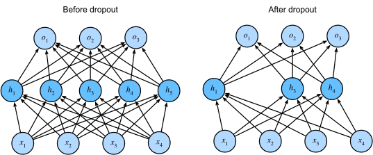
Recall the MLP with a hidden layer and five hidden units from Figure 4.1.1. When we apply dropout to a hidden layer, zeroing out each hidden unit with probability \(p\), the result can be viewed as a network containing only a subset of the original neurons. In Figure 4.6.1, \(h_2\) and \(h_5\) are removed. Consequently, the calculation of the outputs no longer depends on \(h_2\) or \(h_5\) and their respective gradient also vanishes when performing backpropagation. In this way, the calculation of the output layer cannot be overly dependent on any one element of \(h_1, \ldots, h_5\).
Typically, we disable dropout at test time, running the full network with no masking and no rescaling. (The exercises explore one notable exception, keeping dropout on at test time to estimate prediction uncertainty.)
4.6.2 Implementation from Scratch
To implement the dropout function for a single layer, we must draw as many samples from a Bernoulli (binary) random variable as our layer has dimensions, where the random variable takes value \(1\) (keep) with probability \(1-p\) and \(0\) (drop) with probability \(p\). One easy way to implement this is to first draw samples from the uniform distribution \(U[0, 1]\). Then we can keep those nodes for which the corresponding sample is greater than \(p\), dropping the rest.
In the following code, we implement a dropout_layer function that drops out the elements in the tensor input X with probability dropout, rescaling the remainder as described above: dividing the survivors by 1.0-dropout.
def dropout_layer(X, dropout):
    assert 0 <= dropout <= 1
    if dropout == 1: return torch.zeros_like(X)
    mask = (torch.rand_like(X) > dropout).to(X.dtype)
    return mask * X / (1.0 - dropout)
def dropout_layer(X, dropout):
assert 0 <= dropout <= 1
if dropout == 1: return tf.zeros_like(X)
mask = tf.random.uniform(
shape=tf.shape(X), minval=0, maxval=1) < 1 - dropout
return tf.cast(mask, dtype=X.dtype) * X / (1.0 - dropout)def dropout_layer(X, dropout, key):
assert 0 <= dropout <= 1
if dropout == 1: return jnp.zeros_like(X)
mask = jax.random.uniform(key, X.shape) > dropout
return jnp.asarray(mask, dtype=X.dtype) * X / (1.0 - dropout)def dropout_layer(X, dropout):
assert 0 <= dropout <= 1
if dropout == 1: return np.zeros_like(X)
mask = np.random.uniform(0, 1, X.shape) > dropout
return mask.astype(np.float32) * X / (1.0 - dropout)We can test out the dropout_layer function on a few examples. In the following lines of code, we pass our input X through the dropout operation, with probabilities 0, 0.5, and 1, respectively.
X = torch.arange(16, dtype = torch.float32).reshape((2, 8))
print('dropout_p = 0:', dropout_layer(X, 0))
print('dropout_p = 0.5:', dropout_layer(X, 0.5))
print('dropout_p = 1:', dropout_layer(X, 1))
dropout_p = 0: tensor([[ 0., 1., 2., 3., 4., 5., 6., 7.],
[ 8., 9., 10., 11., 12., 13., 14., 15.]])
dropout_p = 0.5: tensor([[ 0., 0., 0., 6., 8., 10., 12., 0.],
[ 0., 18., 20., 22., 24., 0., 28., 0.]])
dropout_p = 1: tensor([[0., 0., 0., 0., 0., 0., 0., 0.],
[0., 0., 0., 0., 0., 0., 0., 0.]])X = tf.reshape(tf.range(16, dtype=tf.float32), (2, 8))
print('dropout_p = 0:', dropout_layer(X, 0))
print('dropout_p = 0.5:', dropout_layer(X, 0.5))
print('dropout_p = 1:', dropout_layer(X, 1))dropout_p = 0: tf.Tensor(
[[ 0. 1. 2. 3. 4. 5. 6. 7.]
[ 8. 9. 10. 11. 12. 13. 14. 15.]], shape=(2, 8), dtype=float32)
dropout_p = 0.5: tf.Tensor(
[[ 0. 0. 4. 6. 8. 10. 12. 0.]
[16. 0. 0. 0. 24. 0. 0. 30.]], shape=(2, 8), dtype=float32)
dropout_p = 1: tf.Tensor(
[[0. 0. 0. 0. 0. 0. 0. 0.]
[0. 0. 0. 0. 0. 0. 0. 0.]], shape=(2, 8), dtype=float32)X = jnp.arange(16, dtype=jnp.float32).reshape(2, 8)
keys = jax.random.split(d2l.get_key(), 3)
print('dropout_p = 0:', dropout_layer(X, 0, keys[0]))
print('dropout_p = 0.5:', dropout_layer(X, 0.5, keys[1]))
print('dropout_p = 1:', dropout_layer(X, 1, keys[2]))dropout_p = 0: [[ 0. 1. 2. 3. 4. 5. 6. 7.]
[ 8. 9. 10. 11. 12. 13. 14. 15.]]
dropout_p = 0.5: [[ 0. 0. 4. 0. 0. 0. 12. 14.]
[ 0. 0. 20. 22. 24. 26. 0. 30.]]
dropout_p = 1: [[0. 0. 0. 0. 0. 0. 0. 0.]
[0. 0. 0. 0. 0. 0. 0. 0.]]X = np.arange(16).reshape(2, 8)
print('dropout_p = 0:', dropout_layer(X, 0))
print('dropout_p = 0.5:', dropout_layer(X, 0.5))
print('dropout_p = 1:', dropout_layer(X, 1))dropout_p = 0: [[ 0. 1. 2. 3. 4. 5. 6. 7.]
[ 8. 9. 10. 11. 12. 13. 14. 15.]]
dropout_p = 0.5: [[ 0. 2. 0. 6. 8. 0. 0. 14.]
[16. 0. 20. 22. 0. 26. 28. 0.]]
dropout_p = 1: [[0. 0. 0. 0. 0. 0. 0. 0.]
[0. 0. 0. 0. 0. 0. 0. 0.]]4.6.2.1 Defining the Model
The model below applies dropout to the output of each hidden layer (following the activation function). We can set dropout probabilities for each layer separately. A common choice is to set a lower dropout probability closer to the input layer. We ensure that dropout is only active during training.
class DropoutMLPScratch(d2l.Classifier):
    def __init__(self, num_outputs, num_hiddens_1, num_hiddens_2,
                 dropout_1, dropout_2, lr):
        super().__init__()
        self.save_hyperparameters()
        self.lin1 = nn.LazyLinear(num_hiddens_1)
        self.lin2 = nn.LazyLinear(num_hiddens_2)
        self.lin3 = nn.LazyLinear(num_outputs)
        self.relu = nn.ReLU()

    def forward(self, X):
        H1 = self.relu(self.lin1(X.reshape((X.shape[0], -1))))
        if self.training:
            H1 = dropout_layer(H1, self.dropout_1)
        H2 = self.relu(self.lin2(H1))
        if self.training:
            H2 = dropout_layer(H2, self.dropout_2)
        return self.lin3(H2)
class DropoutMLPScratch(d2l.Classifier):
def __init__(self, num_outputs, num_hiddens_1, num_hiddens_2,
dropout_1, dropout_2, lr):
super().__init__()
self.save_hyperparameters()
self.lin1 = tf.keras.layers.Dense(num_hiddens_1, activation='relu')
self.lin2 = tf.keras.layers.Dense(num_hiddens_2, activation='relu')
self.lin3 = tf.keras.layers.Dense(num_outputs)
def forward(self, X):
H1 = self.lin1(tf.reshape(X, (tf.shape(X)[0], -1)))
if self.training:
H1 = dropout_layer(H1, self.dropout_1)
H2 = self.lin2(H1)
if self.training:
H2 = dropout_layer(H2, self.dropout_2)
return self.lin3(H2)class DropoutMLPScratch(d2l.Classifier):
def __init__(self, num_outputs, num_hiddens_1, num_hiddens_2,
dropout_1, dropout_2, lr, num_inputs=784, rngs=None):
super().__init__()
self.save_hyperparameters(ignore=['rngs'])
rngs = nnx.Rngs(params=d2l.get_key(), dropout=d2l.get_key()) \
if rngs is None else rngs
self.lin1 = nnx.Linear(num_inputs, num_hiddens_1, rngs=rngs)
self.lin2 = nnx.Linear(num_hiddens_1, num_hiddens_2, rngs=rngs)
self.lin3 = nnx.Linear(num_hiddens_2, num_outputs, rngs=rngs)
self.rngs = rngs
self.deterministic = False
def set_view(self, *, deterministic):
self.deterministic = deterministic
def forward(self, X):
H1 = nnx.relu(self.lin1(X.reshape(X.shape[0], -1)))
if not self.deterministic:
H1 = dropout_layer(H1, self.dropout_1, self.rngs.dropout())
H2 = nnx.relu(self.lin2(H1))
if not self.deterministic:
H2 = dropout_layer(H2, self.dropout_2, self.rngs.dropout())
return self.lin3(H2)class DropoutMLPScratch(d2l.Classifier):
def __init__(self, num_outputs, num_hiddens_1, num_hiddens_2,
dropout_1, dropout_2, lr):
super().__init__()
self.save_hyperparameters()
self.lin1 = nn.Dense(num_hiddens_1, activation='relu')
self.lin2 = nn.Dense(num_hiddens_2, activation='relu')
self.lin3 = nn.Dense(num_outputs)
self.initialize()
def forward(self, X):
H1 = self.lin1(X)
if autograd.is_training():
H1 = dropout_layer(H1, self.dropout_1)
H2 = self.lin2(H1)
if autograd.is_training():
H2 = dropout_layer(H2, self.dropout_2)
return self.lin3(H2)4.6.2.2 Training
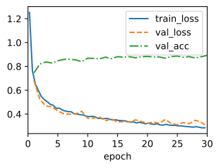
The following is similar to the training of MLPs described previously. Following the convention above, we drop out the layer closer to the input more gently (\(p = 0.2\)) than the deeper one (\(p = 0.5\)).
hparams = {'num_outputs':10, 'num_hiddens_1':256, 'num_hiddens_2':256,
           'dropout_1':0.2, 'dropout_2':0.5, 'lr':0.1}
model = DropoutMLPScratch(**hparams)
data = d2l.FashionMNIST(batch_size=256)
trainer = d2l.Trainer(max_epochs=30)
trainer.fit(model, data)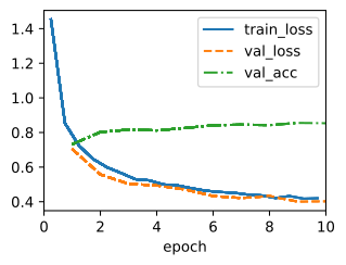
hparams = {'num_outputs':10, 'num_hiddens_1':256, 'num_hiddens_2':256,
           'dropout_1':0.2, 'dropout_2':0.5, 'lr':0.1}
model = DropoutMLPScratch(**hparams)
data = d2l.FashionMNIST(batch_size=256)
trainer = d2l.Trainer(max_epochs=30)
trainer.fit(model, data)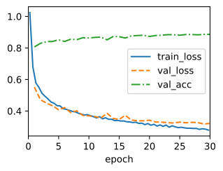
hparams = {'num_outputs':10, 'num_hiddens_1':256, 'num_hiddens_2':256,
           'dropout_1':0.2, 'dropout_2':0.5, 'lr':0.1}
model = DropoutMLPScratch(**hparams)
data = d2l.FashionMNIST(batch_size=256)
trainer = d2l.Trainer(max_epochs=30)
trainer.fit(model, data)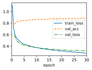
hparams = {'num_outputs':10, 'num_hiddens_1':256, 'num_hiddens_2':256,
           'dropout_1':0.2, 'dropout_2':0.5, 'lr':0.1}
model = DropoutMLPScratch(**hparams)
data = d2l.FashionMNIST(batch_size=256)
# Keep loading in-process: on spawn-based platforms (macOS, Windows) this
# transformed MXNet dataset cannot be pickled for loader workers, and the
# dataset is small enough that parallel loading buys nothing on Linux either.
data.num_workers = 0
trainer = d2l.Trainer(max_epochs=30)
trainer.fit(model, data)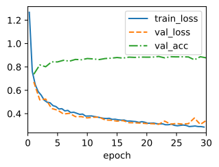
4.6.3 Concise Implementation
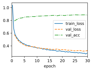
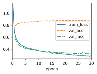
With high-level APIs, we add a Dropout layer after each fully connected layer and pass the dropout probability to its constructor. During training, the Dropout layer will randomly drop out outputs of the previous layer (or equivalently, the inputs to the subsequent layer) according to the specified dropout probability. When not in training mode, the Dropout layer passes the data through unchanged during testing.
class DropoutMLP(d2l.Classifier):
    def __init__(self, num_outputs, num_hiddens_1, num_hiddens_2,
                 dropout_1, dropout_2, lr):
        super().__init__()
        self.save_hyperparameters()
        self.net = nn.Sequential(
            nn.Flatten(), nn.LazyLinear(num_hiddens_1), nn.ReLU(),
            nn.Dropout(dropout_1), nn.LazyLinear(num_hiddens_2), nn.ReLU(),
            nn.Dropout(dropout_2), nn.LazyLinear(num_outputs))
class DropoutMLP(d2l.Classifier):
def __init__(self, num_outputs, num_hiddens_1, num_hiddens_2,
dropout_1, dropout_2, lr):
super().__init__()
self.save_hyperparameters()
self.net = tf.keras.models.Sequential([
tf.keras.layers.Flatten(),
tf.keras.layers.Dense(num_hiddens_1, activation=tf.nn.relu),
tf.keras.layers.Dropout(dropout_1),
tf.keras.layers.Dense(num_hiddens_2, activation=tf.nn.relu),
tf.keras.layers.Dropout(dropout_2),
tf.keras.layers.Dense(num_outputs)])class DropoutMLP(d2l.Classifier):
def __init__(self, num_outputs, num_hiddens_1, num_hiddens_2,
dropout_1, dropout_2, lr, num_inputs=784, rngs=None):
super().__init__()
self.save_hyperparameters(ignore=['rngs'])
rngs = nnx.Rngs(params=d2l.get_key(), dropout=d2l.get_key()) \
if rngs is None else rngs
self.lin1 = nnx.Linear(num_inputs, num_hiddens_1, rngs=rngs)
self.drop1 = nnx.Dropout(dropout_1, rngs=rngs)
self.lin2 = nnx.Linear(num_hiddens_1, num_hiddens_2, rngs=rngs)
self.drop2 = nnx.Dropout(dropout_2, rngs=rngs)
self.lin3 = nnx.Linear(num_hiddens_2, num_outputs, rngs=rngs)
def forward(self, X):
X = X.reshape((X.shape[0], -1))
X = self.drop1(nnx.relu(self.lin1(X)))
X = self.drop2(nnx.relu(self.lin2(X)))
return self.lin3(X)class DropoutMLP(d2l.Classifier):
def __init__(self, num_outputs, num_hiddens_1, num_hiddens_2,
dropout_1, dropout_2, lr):
super().__init__()
self.save_hyperparameters()
self.net = nn.Sequential()
self.net.add(nn.Dense(num_hiddens_1, activation="relu"),
nn.Dropout(dropout_1),
nn.Dense(num_hiddens_2, activation="relu"),
nn.Dropout(dropout_2),
nn.Dense(num_outputs))
self.net.initialize()NNX dropout layers own an RNG stream. Each training call advances that stream, while the evaluation view created by Trainer sets deterministic=True and therefore disables masking. No key needs to be threaded through the loss.
Next, we train the model.
model = DropoutMLP(**hparams)
trainer.fit(model, data)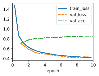
4.6.4 Summary
Inverted dropout replaces each hidden activation \(h\) with a random variable \(h'\) that is zero with probability \(p\) and \(h/(1-p)\) otherwise. The rescaling by \(1/(1-p)\) keeps \(E[h'\mid h] = h\). This is a layerwise statement; after nonlinear downstream layers, the expected network output under dropout need not equal the output of the full network. Dropout is off at test time: the full network runs, with no masking and no rescaling.
Three complementary views explain why dropout helps. The first is noise injection: zeroing activations at random injects noise, and by analogy with Bishop’s input-noise result this favors a smoother learned function (the exact equivalence is proved only for additive input noise, not multiplicative dropout). The second is anti-co-adaptation: because no hidden unit can count on any specific partner being present, each unit is pushed to learn broadly useful features. The third is the historical implicit ensemble interpretation: every training step trains a different thinned subnetwork. The deterministic test-time network is a computational surrogate, not an exact average of their predictions (Srivastava et al. 2014).
Dropout was important for fully connected vision networks of the mid-2010s, but its use now depends on the architecture and training scale. Convolutional networks often rely on data augmentation, normalization (Section 7.3), weight decay, and stochastic depth, using dropout selectively. These methods do not reproduce dropout’s mechanism. Placement matters when dropout and batch normalization are combined. Dropout immediately before batch normalization can perturb the variance used to accumulate running statistics, creating a train–evaluation mismatch in that configuration (Li et al. 2019). Transformer configurations may apply dropout to embeddings, attention and MLP blocks, or output heads, whereas some large-scale models use a rate of zero. Dropout remains a low-cost option that can be combined with weight decay and data augmentation, and it motivated a family of stochastic-regularization methods.
4.6.5 Exercises
[code] Dropout rates and the generalization gap.
DropoutMLPdrops first-layer activations with probability 0.2 and second-layer activations with probability 0.5.- Train the same architecture with both rates set to zero for the same number of epochs, and plot the training and validation loss curves of both runs on the same axes. How does the gap between training and validation loss differ with and without dropout?
Trainercomputes the plotted training loss with the dropout masks active. After training, evaluate the loss of the trainedDropoutMLPon the training set with dropout disabled. Compare the resulting gap with the two gaps from (a).- Swap the two rates, and then set both to 0.5. How do the final validation accuracy and the gap, measured as in (b), change in each case? Which layer tolerates the higher rate?
[code] Activation variance. Let \(h\) be a hidden activation of
DropoutMLPScratchand \(h'\) its value afterdropout_layerwith dropout probability \(p\).- For a fixed \(h\), compute the variance of \(h'\) over the dropout mask. Then let \(h\) vary across the units and examples of a minibatch with mean \(\mu_h\) and variance \(\sigma_h^2\), and express the variance of \(h'\) in terms of \(p\), \(\mu_h\) and \(\sigma_h^2\).
- Train
DropoutMLPScratch(**hparams). After every epoch, pass one fixed validation minibatch through the model with dropout active. For each hidden layer, record the mean and variance of the activations beforedropout_layerand their variance after it. Plot the variances against epochs, and compare the measured ratio of the two variances with your expression from (a).
Ensemble size. A hidden layer with \(n\) units admits \(2^n\) distinct dropout masks, and the ensemble interpretation views each mask as a subnetwork.
- How many distinct joint masks exist across the two hidden layers of 256 units each in
DropoutMLP? - Training runs for 30 epochs over the 60,000 Fashion-MNIST training images, and a fresh mask is drawn for every example. How many joint masks are sampled during training, and what fraction of all joint masks is that?
- Using these two numbers, explain in what sense dropout does, and does not, train an ensemble of all these subnetworks.
- How many distinct joint masks exist across the two hidden layers of 256 units each in
Dropout at test time. ● Dropout is normally disabled at test time, so the full network runs with no masking and no rescaling. Set
dropout_1to zero inDropoutMLP, so that only the second hidden layer is masked. Let \(\mathbf{o}(\mathbf{m})\) and \(\hat{\mathbf{y}}(\mathbf{m})\) be the logits and the softmax output under mask \(\mathbf{m}\), which occurs with probability \(P(\mathbf{m})\). Show that the logits of the unmasked network equal \(\sum_{\mathbf{m}} P(\mathbf{m})\, \mathbf{o}(\mathbf{m})\). Show further that its softmax output equals the normalized weighted geometric mean\[\tilde{y}_j = \frac{\prod_{\mathbf{m}} \hat{y}_j(\mathbf{m})^{P(\mathbf{m})}}{\sum_k \prod_{\mathbf{m}} \hat{y}_k(\mathbf{m})^{P(\mathbf{m})}}. \tag{4.6.2}\]
Explain why neither equality holds in general once
dropout_1is nonzero.[code] Monte Carlo dropout. Instead of disabling dropout at test time, keep it on in the trained
DropoutMLPand run \(T = 20\) forward passes per test example, then average the softmax outputs (Gal and Ghahramani 2016). Compare the resulting accuracy and calibration (the mean largest softmax probability versus the accuracy) against the standard single-pass evaluation.[code] Dropout and weight decay. Weight decay
(Section 2.7) and dropout both regularize
DropoutMLP, but by different mechanisms. Measure each run by its validation accuracy and by the gap between training and validation loss, with both losses evaluated with dropout disabled.- With both dropout rates set to zero, add weight decay as in Section 2.7 at strengths \(\lambda \in \{0, 10^{-4}, 10^{-3}, 10^{-2}\}\). Compare these runs with the dropout-only run at rates 0.2 and 0.5.
- Keep the dropout rates at 0.2 and 0.5, and add weight decay at each nonzero strength from (a). Are the effects of the two regularizers additive, do they show diminishing returns, or do they cancel each other out?
[code] Input dropout. This section applies dropout only to hidden-layer activations. Add dropout on the input features, before the first linear layer, at a small rate such as \(p = 0.1\), keeping the hidden-layer rates unchanged, and compare validation accuracy against the original configuration. Relate the outcome to the redundancy among neighboring pixels.
[code] DropConnect. What happens if we apply dropout to the individual weights of the weight matrix rather than to the activations? This variant is known as DropConnect (Wan et al. 2013). Implement it and compare it against standard dropout on Fashion-MNIST, holding the architecture and training budget fixed.
[code] First-layer features. Train
DropoutMLPand a copy with both dropout rates set to zero, then visualize each first-layer unit’s incoming weight vector as a \(28 \times 28\) image. Compare at least 16 units side by side for each model, as Figure 7 of Srivastava et al. (2014) does for an autoencoder on MNIST. Describe how the two sets of images differ in noise and in redundancy across units.[code] Custom noise injection. ● Invent a technique for injecting random noise during training that differs from both dropout and DropConnect, for example additive Gaussian noise on the activations, or randomly rescaling rather than zeroing each unit’s output. State the randomization rule and any rescaling needed to preserve the expectation of each activation. Implement the method and train it at two or three noise levels on Fashion-MNIST, with the same architecture and epoch budget as
DropoutMLP. Compare the validation accuracy and the gap between training and validation loss at each noise level with those ofDropoutMLP.