%matplotlib inline
from d2l import torch as d2l
import torch
from torch import nn8.1 Working with Sequences
The models developed so far usually map one fixed-shape feature vector \(\mathbf{x}\in\mathbb{R}^d\) to one output and optimize an average over examples. A sequence model must additionally preserve order within an example and accept lengths that may differ. We now work with sequences: ordered lists of feature vectors \(\mathbf{x}_1, \dots, \mathbf{x}_T\), where the index \(t \in \mathbb{Z}^+\) is a time step and neighboring entries may be statistically dependent.
%matplotlib inline
from d2l import tensorflow as d2l
import tensorflow as tf%matplotlib inline
from d2l import jax as d2l
import jax
from jax import numpy as jnp
import numpy as np%matplotlib inline
from d2l import mxnet as d2l
from mxnet import autograd, np, npx, gluon, init
from mxnet.gluon import nn
npx.set_np()8.1.1 Sequential Data and Its Challenges
Consider text completion. The distribution of the next word changes with the preceding words, which lets an email client predict a continuation better than it could from marginal word frequencies alone. Text can be represented as a sequence of characters or words. Audio, whether speech or music, is a sequence of samples, or of the spectrogram frames a model actually consumes. Time series such as prices, sensor readings, and patient vitals arrive one measurement at a time, each shaped by its recent past.
What these examples share is that order and dependence can carry predictive information. We still assume that entire sequences (a whole document, a whole patient trajectory) are drawn independently from a fixed distribution over sequences. But within a sequence the entries are not independent: the medicine a patient receives on day ten of a hospital stay depends heavily on the previous nine days. If entries were independent, conditioning on neighboring entries would not improve prediction, although the marginal distribution could still be learned.
Dependence also means that order carries information and that a sequence’s statistics can drift: a document reads differently at its end than at its beginning, and a patient’s status evolves toward recovery or decline. We therefore do not assume independence, or even that the per-step statistics stay fixed over time; we assume only that whole sequences come from one fixed distribution over sequences.
Prediction tasks over sequences come in a few shapes. Sometimes the target is a single label for an entire input sequence (the sentiment of a movie review), sometimes a sequence given a fixed input (captioning an image), and sometimes a sequence given a sequence (translating a sentence, transcribing speech). Before handling targets of any kind, we tackle the most basic version: modeling the sequence itself, that is, estimating how probable a given sequence is, \(P(\mathbf{x}_1, \ldots, \mathbf{x}_T)\). The later sections build on this probability model.
8.1.2 Autoregressive Models
We begin by predicting each entry from the preceding observations. Given a numerical series such as a stock index or a temperature reading, a forecaster who wants to act on the next step cares about the conditional distribution
\[P(x_t \mid x_{t-1}, \ldots, x_1). \tag{8.1.1}\]
Even when the full distribution is hard to pin down, a useful summary is the conditional expectation \(\mathbb{E}[x_t \mid x_{t-1}, \ldots, x_1]\), which we could try to fit with, say, linear regression (Section 2.1). A model that regresses a signal on its own past is an autoregressive model: features and target are drawn from the same series.
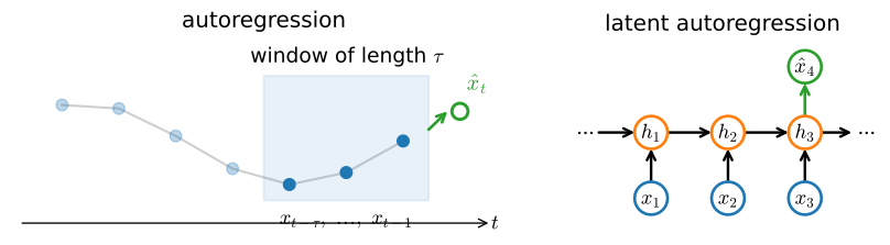
There is an immediate obstacle. The number of conditioning inputs \(x_{t-1}, \ldots, x_1\) grows with \(t\), so if we treat the history as a training set, every example has a different number of features and no fixed-input model applies. Two strategies produce fixed-size representations of the history (Figure 8.1.1).
8.1.2.1 Fixed Windows
The first strategy is to condition only on the last \(\tau\) observations \(x_{t-1}, \ldots, x_{t-\tau}\), discarding older history. Now every example has exactly \(\tau\) features (for \(t > \tau\)), so any fixed-length model, linear or deep, applies directly. This is autoregression in its narrow sense.
This fixed window is exactly the idea behind the n-gram language models of Section 8.3, where the signal is a stream of words, and, much later, behind the fixed context window an attention model reads all at once. A window is simple and easy to parallelize; its weakness is a hard horizon, since anything older than \(\tau\) steps is invisible to the model.
8.1.2.2 Latent Summaries
The second strategy keeps a running summary \(h_t\) of everything seen so far and updates it as new observations arrive. We predict from the summary, \(\hat{x}_t = P(x_t \mid h_t)\), and refresh it with \(h_t = g(h_{t-1}, x_{t-1})\). Because \(h_t\) is never observed directly, this is a latent autoregressive model. The state \(h_t\) has fixed size no matter how long the history, so the whole unbounded past is compressed into bounded memory.
This latent-state picture is exactly the recurrent neural network we build in Section 8.4, and, in a linearized form, the state space models of Chapter 12. The next two chapters examine what the state \(h_t\) should retain and how it should be updated.
8.1.2.3 From Conditionals to Sequences
Whichever strategy we pick, the per-step conditionals compose into a model of the whole sequence. By the chain rule of probability,
\[P(x_1, \ldots, x_T) = P(x_1) \prod_{t=2}^T P(x_t \mid x_{t-1}, \ldots, x_1), \tag{8.1.2}\]
so an autoregressive model of the next entry is automatically a model of the entire sequence: to score a sequence, multiply the conditionals; to generate one, sample them left to right. When the entries are discrete tokens, each conditional is a classifier over the vocabulary, and estimating \(P(x_1, \ldots, x_T)\) is exactly language modeling (Section 8.3). For now we keep the values continuous and focus on prediction.
8.1.3 Markov Models and Stationarity
The fixed-window strategy carries a hidden assumption worth naming.
8.1.3.1 The Markov Condition
When conditioning on the last \(\tau\) steps loses no predictive power relative to the full history, we say the sequence satisfies a Markov condition: the future is conditionally independent of the distant past given the recent past. With \(\tau = 1\) the series follows a first-order Markov model, and with \(\tau = k\) a \(k^{\textrm{th}}\)-order one. Under the first-order condition the joint factorization collapses to a product over adjacent pairs:
\[P(x_1, \ldots, x_T) = P(x_1) \prod_{t=2}^T P(x_t \mid x_{t-1}). \tag{8.1.3}\]
In practice the Markov condition rarely holds exactly. Real text keeps yielding information as we widen the context, but with sharply diminishing returns, so it is often worth pretending a \(k^{\textrm{th}}\)-order condition holds in order to buy computational and statistical tractability. Even today’s large language models condition on at most thousands of tokens at a time, not their entire training history. For discrete data the simplest such model just counts: \(P(x_t \mid x_{t-1})\) is estimated by the relative frequency of each successor, an idea we take up again for n-grams in Section 8.3.
8.1.3.2 Stationarity
Fitting any of these models presupposes that the rule generating each entry from its predecessors does not itself change over time. Dynamics with this property are called stationary. The values still change, sometimes dramatically; what stays put is the conditional law \(P(x_t \mid x_{t-1}, \ldots)\). Stationarity is what lets us pool examples from different parts of one sequence, or from many sequences, into a single training set, and it is why we build training data by sampling windows.
One choice above was implicit: we factored the sequence left to right. Any order gives a valid factorization, but for causal data the forward direction is usually easier to learn, since predicting an effect from its cause tends to be simpler than the reverse (Peters et al. 2017). As we generally want to predict the future from the past anyway, left to right it is.
8.1.4 Training
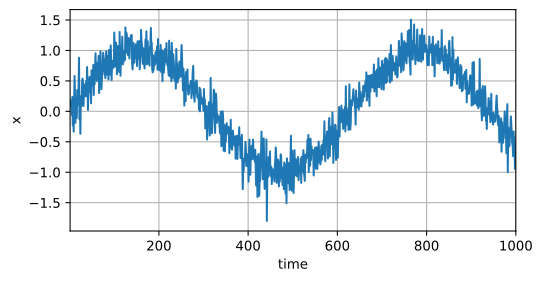
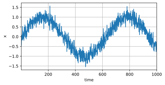
The fixed-window objective now permits a controlled comparison between one-step prediction and recursive rollout. We work first with continuous synthetic data, where we control the ground truth. We draw 1000 points from the sine of 0.01 times the time step, corrupt each with additive noise, and carve training examples out of the result.
class Data(d2l.DataModule):
    def __init__(self, batch_size=16, T=1000, num_train=600, tau=4):
        self.save_hyperparameters()
        self.time = d2l.arange(1, T + 1, dtype=d2l.float32)
        self.x = d2l.sin(0.01 * self.time) + d2l.randn(T) * 0.2
class Data(d2l.DataModule):
def __init__(self, batch_size=16, T=1000, num_train=600, tau=4):
self.save_hyperparameters()
self.time = d2l.arange(1, T + 1, dtype=d2l.float32)
self.x = d2l.sin(0.01 * self.time) + d2l.normal([T]) * 0.2class Data(d2l.DataModule):
def __init__(self, batch_size=16, T=1000, num_train=600, tau=4):
self.save_hyperparameters()
self.time = d2l.arange(1, T + 1, dtype=d2l.float32)
key = d2l.get_key()
self.x = d2l.sin(0.01 * self.time) + jax.random.normal(key,
[T]) * 0.2class Data(d2l.DataModule):
def __init__(self, batch_size=16, T=1000, num_train=600, tau=4):
self.save_hyperparameters()
self.time = d2l.arange(1, T + 1, dtype=d2l.float32)
self.x = d2l.sin(0.01 * self.time) + d2l.randn(T) * 0.2data = Data()
d2l.plot(data.time, data.x, 'time', 'x', xlim=[1, 1000], figsize=(6, 3))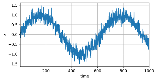
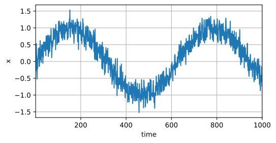
To turn the series into supervised examples, we adopt the fixed-window strategy with a window of length \(\tau\): the label is \(y = x_t\) and the features are \(\mathbf{x}_t = [x_{t-\tau}, \ldots, x_{t-1}]\). This yields \(T - \tau\) examples, since the first \(\tau\) steps lack enough history and we drop them (padding with zeros is the alternative). We create a data iterator over the first 600 examples, covering a bit less than one period of the sine.
@d2l.add_to_class(Data)
def get_dataloader(self, train):
    features = [self.x[i : self.T-self.tau+i] for i in range(self.tau)]
    self.features = d2l.stack(features, 1)
    self.labels = d2l.reshape(self.x[self.tau:], (-1, 1))
    i = slice(0, self.num_train) if train else slice(self.num_train, None)
    return self.get_tensorloader([self.features, self.labels], train, i)
Our model is a plain linear regression on the \(\tau\) lag features, about the simplest autoregressive model there is.
model = d2l.LinearRegression(lr=0.01)
trainer = d2l.Trainer(max_epochs=5)
trainer.fit(model, data)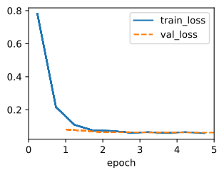
model = d2l.LinearRegression(lr=0.01)
trainer = d2l.Trainer(max_epochs=5)
trainer.fit(model, data)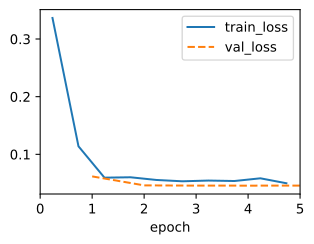
model = d2l.LinearRegression(num_inputs=data.tau, lr=0.01)
trainer = d2l.Trainer(max_epochs=5)
trainer.fit(model, data)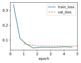
model = d2l.LinearRegression(lr=0.01)
trainer = d2l.Trainer(max_epochs=5)
trainer.fit(model, data)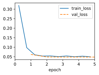
8.1.5 Prediction
8.1.5.1 One-Step-Ahead Prediction
First the easy case: predict \(\hat{x}_t\) from the true previous \(\tau\) values.
onestep_preds = d2l.numpy(model(data.features))
d2l.plot(data.time[data.tau:], [data.labels, onestep_preds], 'time', 'x',
         legend=['labels', '1-step preds'], figsize=(6, 3))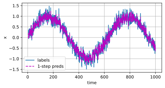
onestep_preds = d2l.numpy(model(data.features))
d2l.plot(data.time[data.tau:], [data.labels, onestep_preds], 'time', 'x',
         legend=['labels', '1-step preds'], figsize=(6, 3))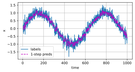
onestep_preds = model(data.features)
d2l.plot(data.time[data.tau:], [data.labels, onestep_preds], 'time', 'x',
         legend=['labels', '1-step preds'], figsize=(6, 3))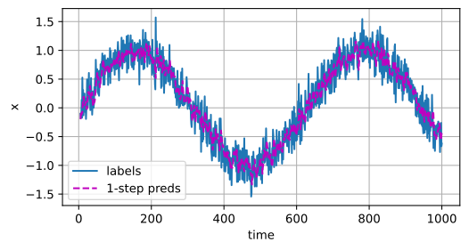
onestep_preds = d2l.numpy(model(data.features))
d2l.plot(data.time[data.tau:], [data.labels, onestep_preds], 'time', 'x',
         legend=['labels', '1-step preds'], figsize=(6, 3))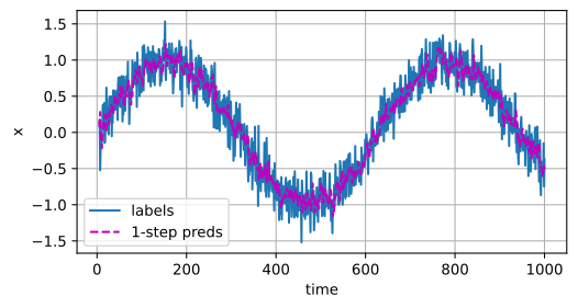
These predictions track the series closely, even near the end at \(t = 1000\).
8.1.5.2 Multistep Rollout
The hard case is forecasting several steps ahead. Suppose we have observed only up to step 604 (num_train + tau) and want to predict \(\hat{x}_{609}\). We cannot form the one-step input for step 609, because we have not observed \(x_{605}, \ldots, x_{608}\). The fix is to feed our own predictions back in as if they were observations, rolling forward one step at a time:
\[\begin{aligned} \hat{x}_{605} &= f(x_{601}, x_{602}, x_{603}, x_{604}), \\ \hat{x}_{606} &= f(x_{602}, x_{603}, x_{604}, \hat{x}_{605}), \\ \hat{x}_{607} &= f(x_{603}, x_{604}, \hat{x}_{605}, \hat{x}_{606}),\\ \hat{x}_{608} &= f(x_{604}, \hat{x}_{605}, \hat{x}_{606}, \hat{x}_{607}),\\ \hat{x}_{609} &= f(\hat{x}_{605}, \hat{x}_{606}, \hat{x}_{607}, \hat{x}_{608}),\\ &\vdots\end{aligned} \tag{8.1.4}\]
For an observed series \(x_1, \ldots, x_t\), the prediction \(\hat{x}_{t+k}\) is the \(k\)-step-ahead prediction, and a rollout chains one-step predictions to reach it. Let us see how it goes.
multistep_preds = d2l.zeros(data.T)
multistep_preds[:] = data.x
for i in range(data.num_train + data.tau, data.T):
    multistep_preds[i] = model(
        d2l.reshape(multistep_preds[i-data.tau : i], (1, -1)))
multistep_preds = d2l.numpy(multistep_preds)
multistep_preds = tf.Variable(d2l.zeros(data.T))
multistep_preds[:].assign(data.x)
for i in range(data.num_train + data.tau, data.T):
multistep_preds[i].assign(d2l.reshape(model(
d2l.reshape(multistep_preds[i-data.tau : i], (1, -1))), ()))multistep_preds = d2l.zeros(data.T)
multistep_preds = multistep_preds.at[:].set(data.x)
for i in range(data.num_train + data.tau, data.T):
pred = model(d2l.reshape(
multistep_preds[i-data.tau : i], (1, -1)))
multistep_preds = multistep_preds.at[i].set(pred.item())multistep_preds = d2l.zeros(data.T)
multistep_preds[:] = data.x
for i in range(data.num_train + data.tau, data.T):
multistep_preds[i] = model(
d2l.reshape(multistep_preds[i-data.tau : i], (1, -1)))
multistep_preds = d2l.numpy(multistep_preds)d2l.plot([data.time[data.tau:], data.time[data.num_train+data.tau:]],
[onestep_preds, multistep_preds[data.num_train+data.tau:]], 'time',
'x', legend=['1-step preds', 'multistep preds'], figsize=(6, 3))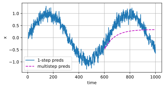
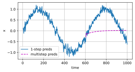
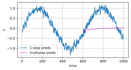
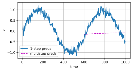
The forecast collapses to a near-constant within a few steps. The reason is error accumulation. Say that after one step we have some error \(\epsilon_1 = \bar\epsilon\). That error now perturbs the input of the next step, so we incur an error of about \(\epsilon_2 = \bar\epsilon + c\,\epsilon_1\) for some constant \(c\), and so on: small mistakes compound as they are fed back, and the prediction diverges rapidly from the truth. You have seen this before: a weather forecast is sharp a day out and nearly useless two weeks out.
To watch the degradation set in, we compute \(k\)-step predictions across the whole series for \(k = 1, 4, 16, 64\).
def k_step_pred(k):
    features = []
    for i in range(data.tau):
        features.append(data.x[i : i+data.T-data.tau-k+1])
    # The (i+tau)-th element stores the (i+1)-step-ahead predictions
    for i in range(k):
        preds = model(d2l.stack(features[i : i+data.tau], 1))
        features.append(d2l.reshape(preds, -1))
    return features[data.tau:]
def k_step_pred(k):
features = []
for i in range(data.tau):
features.append(data.x[i : i+data.T-data.tau-k+1])
# The (i+tau)-th element stores the (i+1)-step-ahead predictions
for i in range(k):
preds = model(d2l.stack(features[i : i+data.tau], 1))
features.append(d2l.reshape(preds, -1))
return features[data.tau:]def k_step_pred(k):
features = []
for i in range(data.tau):
features.append(data.x[i : i+data.T-data.tau-k+1])
# The (i+tau)-th element stores the (i+1)-step-ahead predictions
for i in range(k):
preds = model(d2l.stack(features[i : i+data.tau], 1))
features.append(d2l.reshape(preds, -1))
return features[data.tau:]def k_step_pred(k):
features = []
for i in range(data.tau):
features.append(data.x[i : i+data.T-data.tau-k+1])
# The (i+tau)-th element stores the (i+1)-step-ahead predictions
for i in range(k):
preds = model(d2l.stack(features[i : i+data.tau], 1))
features.append(d2l.reshape(preds, -1))
return features[data.tau:]steps = (1, 4, 16, 64)
preds = k_step_pred(steps[-1])
d2l.plot(data.time[data.tau+steps[-1]-1:],
[d2l.numpy(preds[k-1]) for k in steps], 'time', 'x',
legend=[f'{k}-step preds' for k in steps], figsize=(6, 3))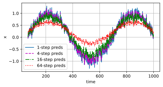
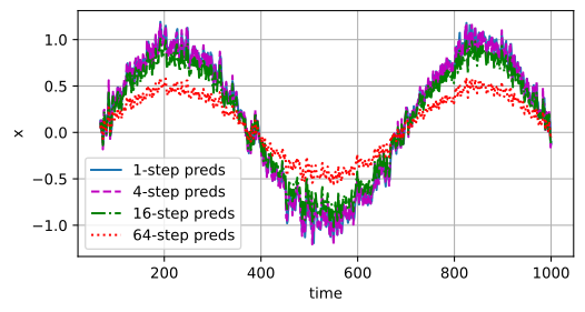
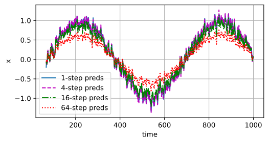
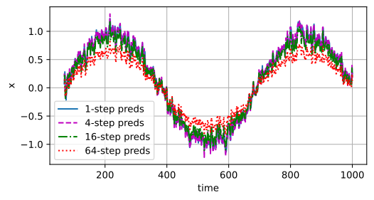
The 1- and 4-step forecasts still hug the truth; the 16-step forecast is visibly damped, and by 64 steps the accumulated error has shrunk the prediction to a low-amplitude echo of the real series.
8.1.5.3 Error Accumulation in Autoregressive Rollouts
This compounding can occur whenever an autoregressive generator consumes its own outputs: prediction errors change the context used by later steps. A language model that samples one token at a time can drift off topic or into repetition once a few odd choices steer it into a region of text it never saw during training; a learned world model simulating an environment loses coherence over a long rollout for the same reason. Two remedies run through the rest of the book. First, how we turn each conditional into a concrete next value matters: choosing well at each step (the decoding strategies of Section 8.7) keeps a rollout on the manifold of realistic sequences far longer than blindly taking the mean or mode. Second, exposing a model to its own predictions during training, not only to gold histories, narrows the gap between the one-step world it is trained in and the multistep world it is used in. We return to both.
8.1.6 Summary
Sequences break the i.i.d. assumption: entries within a sequence are dependent, and the values are often nonstationary even when the underlying dynamics are stationary. Autoregressive models turn sequence modeling into ordinary supervised learning by predicting each entry from its predecessors, either through a fixed window of the last \(\tau\) observations (autoregression, the n-gram idea) or through a recurrent latent state that summarizes the whole past in bounded memory (latent autoregression, the RNN idea). One-step-ahead prediction is comparatively easy; multistep forecasting must feed predictions back as inputs, so it accumulates error and degrades quickly. Respect temporal order when training, never on future data, and expect extrapolation to be much harder than interpolation.
8.1.7 Exercises
- [code] Window length.
Datasuppliestau=4lag features andd2l.LinearRegressionfits them.- Increase
tauand retrain. How many past observations are needed before the validation error stops improving? - Suppose the noise term in
Datawere removed. How many past observations then suffice for exact prediction, and why?
- Increase
- [code] Dilated and averaged lags. ● Keep four features for
d2l.LinearRegressionbut let them reach further back: once as the lags \(x_{t-1}, x_{t-2}, x_{t-4}, x_{t-8}\), and once as the four block means \(\frac{1}{4}\sum_{i=0}^{3} x_{t-4j+i}\) for \(j = 1, \ldots, 4\). Compare their validation errors with those for \(\tau = 4\) and \(\tau = 16\). Which construction helps, and why? - [code] Nonlinear autoregressor. Replace
d2l.LinearRegressionby a small MLP on the same four lag features and retrain, possibly for more epochs. How do the one-step and the multistep predictions change? - [code] Error growth with the horizon. For each \(k\), the last entry of the list that
k_step_pred(k)returns holds the \(k\)-step-ahead predictions ofdata.x[data.tau+k-1:].- For \(k \in \{1, 2, 4, \ldots, 256\}\), plot the mean squared \(k\)-step error against \(k\) on a logarithmic axis. Where does the curve bend upward, and how does the bend relate to the damping of the 16-step and 64-step forecasts?
- The variance of the series is the mean squared error of a forecast that always predicts the series mean. Find the smallest \(k\) at which the mean squared \(k\)-step error exceeds this variance. What does a forecast beyond this horizon offer over the constant forecast?
- [code] Regime switching. ● Replace the single sine in
Databy a series that alternates between \(\sin(0.01\,t)\) and \(\sin(0.05\,t)\) every 200 time steps, and keep the additive noise. Both regimes then occur among the training examples and among the validation examples. The switching series violates the stationarity assumption of Section 8.1.3.2. Does one linear model with \(\tau = 4\) nevertheless fit both regimes, and why? Report training and validation error for each regime separately and locate the positions along the series where the fit is worst. - [code] Scheduled sampling. ● Section 8.1.5.3 states that exposing a model to its own predictions during training narrows the gap between one-step training and multistep use. Test the claim with a variant of scheduled sampling (Bengio et al. 2015) for the linear model with \(\tau = 4\). In every minibatch, replace each lag feature with probability \(\epsilon\) by the model’s current one-step prediction of that observation. Train one model for each \(\epsilon \in \{0, 0.25, 0.5, 1\}\). For each model, measure the one-step validation error and the mean squared error of the last entry of
k_step_pred(64). Does any \(\epsilon > 0\) lower the 64-step error below its value at \(\epsilon = 0\)? How does the one-step error change? - Momentum strategies. An investor selects stocks by their own past returns, expecting those that rose to keep rising. State the assumption about the return series that this strategy requires, in the terms of Section 8.1.3.1 and Section 8.1.3.2, and describe one mechanism by which the assumption fails.