4.5 Generalization in Deep Learning
Earlier chapters related generalization to model complexity, but the raw number of parameters is an unreliable capacity measure for deep networks. Networks can interpolate a training set and still generalize, and different optimizers can select different solutions from the same parameterized family. No single theory accounts for all such behavior.
This section develops one bounded conclusion: parameter count alone does not predict test error. Double descent supplies empirical and tractable-model evidence near the interpolation threshold; implicit regularization explains why the training algorithm also matters. Early stopping and grokking are then presented as consequences of this dependence on optimization time, not as a catalogue of universal laws.
4.5.1 Revisiting Overfitting and Regularization
According to the “no free lunch” theorem of Wolpert (1996), any learning algorithm generalizes better on some data distributions and worse on others. Thus, given a finite training set, a model must rely on assumptions, or inductive biases. Effective inductive biases often reflect known structure in the data. They express preferences for solutions with particular properties. For example, a deep MLP favors complicated functions formed by composing simpler functions.
With machine learning models encoding inductive biases, our approach to training them typically consists of two phases: (i) fit the training data; and (ii) estimate the generalization error (the true error on the underlying population) by evaluating the model on holdout data. The difference between our fit on the training data and our fit on the test data is called the generalization gap (Section 2.6) and when this is large, we say that our models overfit to the training data. In extreme cases of overfitting, we might exactly fit the training data, even when the test error remains significant. And in the classical view, the interpretation is that our models are too complex, requiring that we either shrink the number of features, the number of nonzero parameters learned, or the size of the parameters as quantified by their norm. Recall the plot of model complexity compared with loss (Figure 2.6.1) from Section 2.6.
However deep learning complicates this picture in counterintuitive ways. First, some modern classification models are expressive enough to fit every training example in large datasets (Zhang et al. 2021). In the classical picture, we might think that this setting lies on the far right extreme of the model complexity axis, and that any improvements in generalization error must come by way of regularization, either by reducing the complexity of the model class, or by applying a penalty, severely constraining the set of values that our parameters might take. Deep learning does not always follow this classical pattern.
For many deep learning benchmarks, several candidate architectures can reach nearly zero training error. Their useful differences then appear in validation error, compute, or other deployment criteria. In some such regimes, despite fitting the training data perfectly, we can actually reduce the generalization error further by making the model even more expressive, e.g., adding layers, nodes, or training for a larger number of epochs. The relationship between the generalization gap and model complexity (as measured, for example, by network depth or width) can also be nonmonotonic: additional complexity initially hurts and subsequently helps in a “double-descent” pattern (Belkin et al. 2019; Nakkiran et al. 2021), which we examine below. Consequently, methods used to mitigate overfitting may either restrict a model or make it more expressive.
Complicating things even further, while the guarantees provided by classical learning theory can be conservative even for classical models, they appear powerless to explain why deep neural networks generalize in the first place. Because deep neural networks are capable of fitting arbitrary labels even for large datasets, and despite the use of familiar methods such as \(\ell_2\) regularization, worst-case complexity bounds are often vacuous at modern scales when they depend only on the full hypothesis class, as basic parameter-count VC bounds do. More data-dependent and algorithm-dependent bounds remain an active research area; no single account yet predicts deep-network generalization across settings. (Section 3.6 introduces these ideas; the mechanics of the classical bounds (concentration of measure, uniform convergence, and Rademacher complexity, with proofs) are developed in Section 27.6.)
4.5.1.1 Double Descent
Double descent is one observed departure from the simplest classical picture. Classical theory predicts a U-shaped test-error curve: as we add capacity, error first falls (we stop underfitting) and then rises (we begin overfitting), with an intermediate optimum (recall Figure 2.6.1 from Section 2.6). In some models, datasets, and training regimes, test error instead shows double descent. Near the interpolation threshold, the smallest capacity at which the training procedure fits the data, test error rises and may then descend a second time as capacity increases. Parameter count can locate this threshold in simple linear models, but it is not a reliable proxy for the effective capacity of a deep network. This non-monotone, two-valley shape is called double descent (Belkin et al. 2019), and it appears when we grow the model, when we train for more epochs, and when we add more data (Nakkiran et al. 2021) (Figure 4.5.1).
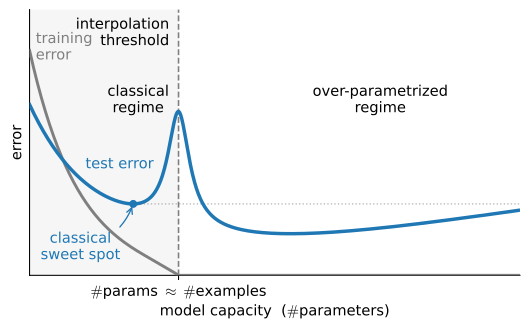
Why can bigger be better past the point of interpolation? In linear least-squares and random-feature models, the minimum-norm interpolant can have high variance near a rank transition and lower variance after more features create additional interpolating solutions. This mechanism gives a precise double-descent calculation, but it is a model-specific explanation rather than a theorem about all deep networks. Section 27.6 develops that calculation; we return below to what is known about optimizer-dependent implicit bias.
Model size, moreover, is only one of three knobs that trace out this curve. Nakkiran et al. (2021) document model-wise double descent (grow the network, the flavor above and the one the appendix analyzes), epoch-wise double descent (fix the network and train longer: test error falls, rises as the model begins to interpolate noise, then falls again), and sample-wise double descent: adding training examples can hurt test performance, because more data moves the interpolation threshold and can push a fixed model back into the high-variance spike. All three are organized by a single axis that Nakkiran et al. call effective model complexity, roughly how many examples the full training procedure (model, optimizer, and budget) can fit perfectly. The error peaks wherever that quantity crosses the dataset size. This chapter only names the phenomena; the appendix proves the model-wise case, and the exercises below let you produce the epoch-wise one yourself.
4.5.2 Inspiration from Nonparametrics
Approaching deep learning for the first time, it is tempting to think of deep networks as parametric models. After all, the models do have millions of parameters. When we update the models, we update their parameters. When we save the models, we write their parameters to disk. However, mathematics and computer science are riddled with counterintuitive changes of perspective, and surprising isomorphisms between seemingly different problems. While neural networks clearly have parameters, in some ways it can be more fruitful to think of them as behaving like nonparametric models. So what precisely makes a model nonparametric? While the name covers a diverse set of approaches, one common theme is that nonparametric methods tend to have a level of complexity that grows as the amount of available data grows.
Perhaps the simplest example of a nonparametric model is the \(k\)-nearest neighbor algorithm (we will cover more nonparametric models later, for example in Section 10.1.3). Here, at training time, the learner retains the dataset. Then, at prediction time, when confronted with a new point \(\mathbf{x}\), the learner looks up the \(k\) nearest neighbors (the \(k\) points \(\mathbf{x}_i'\) that minimize some distance \(d(\mathbf{x}, \mathbf{x}_i')\)). When \(k=1\), this algorithm is called \(1\)-nearest neighbors, and it achieves zero training error when training inputs are distinct and ties are resolved in favor of the queried example. That, however, does not mean that the algorithm will not generalize. Under suitable conditions, the error of the \(1\)-nearest neighbor rule comes within a factor of two of the optimal (Bayes) error as the dataset grows (Cover and Hart 1967), and it is optimal in the noiseless case where the Bayes error is zero. (Full consistency, convergence to the optimal predictor, requires \(k\)-nearest neighbors with \(k \to \infty\) while \(k/n \to 0\).)
Note that \(1\)-nearest neighbor requires that we specify some distance function \(d\), or equivalently, that we specify some vector-valued basis function \(\phi(\mathbf{x})\) for featurizing our data. The zero-training-error statement assumes distinct training inputs and a rule for ties. The limiting Cover–Hart guarantee also requires a suitable metric space and regularity conditions connecting nearby inputs to their label distributions; an arbitrary or degenerate distance need not satisfy it. Under those conditions, \(1\)-nearest neighbor approaches its near-optimal limit, but different distance metrics \(d\) encode different inductive biases and, with a finite amount of available data, will yield different predictors. Different choices of the distance metric \(d\) represent different assumptions about the underlying patterns and the performance of the different predictors will depend on how compatible the assumptions are with the observed data.
In a sense, because neural networks are over-parametrized, possessing many more parameters than are needed to fit the training data, they tend to interpolate the training data (fitting it perfectly) and thus behave, in some ways, more like nonparametric models. More recent theoretical research has established deep connection between large neural networks and nonparametric methods, notably kernel methods. In particular, Jacot et al. (2018) demonstrated that in the limit, as multilayer perceptrons with randomly initialized weights grow infinitely wide, they become equivalent to (nonparametric) kernel methods for a specific choice of the kernel function (essentially, a distance function), which they call the neural tangent kernel. While current neural tangent kernel models may not fully explain the behavior of modern deep networks, their success as an analytical tool shows how a nonparametric limit can help in understanding the behavior of over-parametrized deep networks.
4.5.3 Early Stopping
While deep neural networks are capable of fitting arbitrary labels, even when labels are assigned incorrectly or randomly (Zhang et al. 2021), this capability only emerges over many iterations of training. A line of work (Arpit et al. 2017; Rolnick et al. 2017) has shown that in the setting of label noise, neural networks tend to fit cleanly labeled data first and only subsequently to interpolate the mislabeled data. Moreover, this phenomenon can be turned into a generalization bound: if a model fits the clean examples but not deliberately mislabeled ones added to the training set, one can certify (with high probability) that its population error is small (Garg et al. 2021).
Together these findings help to motivate early stopping, a classic technique for regularizing deep neural networks. Here, rather than directly constraining the values of the weights, one constrains the number of epochs of training. The most common way to determine the stopping criterion is to monitor validation error throughout training (typically by checking once after each epoch) and to cut off training when the validation error has not decreased by more than some small amount \(\epsilon\) for some number of epochs. This is sometimes called a patience criterion. Besides its potential to improve generalization in the setting of noisy labels, early stopping also saves time: once the patience criterion is met, one can terminate training. For large models that might require days of training simultaneously across eight or more GPUs, well-tuned early stopping can save researchers days of time and can save their employers many thousands of dollars.
Early stopping often helps when continued optimization begins to fit label noise. Its effect is not determined by label noise alone: model mismatch, optimization dynamics, augmentation, and the validation criterion also matter. Natural image tasks such as distinguishing cats from dogs should not be assumed realizable. Treat the stopping epoch as a hyperparameter selected on validation data, and retain the parameters from the best validated epoch rather than the last epoch examined.
4.5.4 Classical Regularization Methods for Deep Networks
In Chapter 2, we described several classical regularization techniques for constraining the complexity of our models. In particular, Section 2.7 introduced a method called weight decay, which consists of adding a regularization term to the loss function in order to penalize large values of the weights. Depending on which weight norm is penalized this technique is known either as ridge regularization (for \(\ell_2\) penalty) or lasso regularization (for an \(\ell_1\) penalty). The classical analysis treats them as restricting the values that the weights can take enough to prevent the model from fitting arbitrary labels.
In deep learning implementations, weight decay remains a popular tool. However, researchers have noted that typical strengths of \(\ell_2\) regularization are insufficient to prevent the networks from interpolating the data (Zhang et al. 2021). Their effects cannot be reduced to preventing interpolation. Depending on the model and optimizer, weight decay changes parameter norms, margins, effective learning rates, and the trajectory through parameter space. Early stopping is a separate control on that trajectory. Like the number of layers or the distance metric in 1-nearest neighbor, these choices may improve generalization by encoding inductive biases compatible with the patterns found in datasets of interest. Thus, classical regularizers remain popular in deep learning implementations, even if the theoretical rationale for their efficacy may be radically different.
4.5.4.1 Implicit Regularization
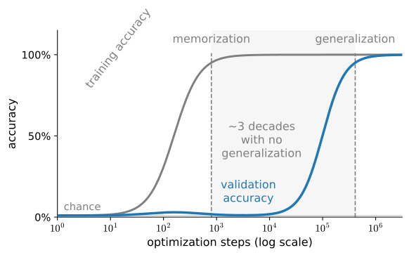
A learning algorithm imposes an implicit bias: among many interpolating parameters, its initialization and update rule make some solutions more likely than others. The bias is understood sharply in a few model classes. For linearly separable data, gradient descent on the logistic loss provably converges in direction to the \(\ell_2\) maximum-margin separator, even with no explicit penalty (Soudry et al. 2018). This theorem concerns a linear predictor and does not establish that SGD finds small-norm or well-generalizing solutions in an arbitrary deep network. Likewise, raw parameter-space flatness changes under function-preserving reparameterizations, so it cannot by itself explain generalization (Dinh et al. 2017). Sharpness-aware minimization is a useful training method (Foret et al. 2021), but its success does not turn flatness into a parameterization-invariant theory. Weight decay and early stopping interact with these algorithmic biases; their effects must be measured rather than inferred from the linear theorem. Grokking illustrates this: on small algorithmic tasks, networks first memorize the training set and only much later, after many further steps of training, suddenly generalize, a reminder that optimization dynamics govern generalization as much as architecture (Power et al. 2022). Figure 4.5.2 shows the signature: training accuracy saturates almost immediately, while validation accuracy sits at chance for orders of magnitude more steps before snapping to near-perfect, long after any conventional early-stopping rule would have given up.
Notably, deep learning researchers have also built on techniques first popularized in classical regularization contexts, such as adding noise to model inputs. In the next section we will introduce the famous dropout technique (invented by Srivastava et al. (2014)), which has become a mainstay of deep learning, even as the theoretical basis for its efficacy remains similarly mysterious.
4.5.5 Summary
Unlike classical linear models, which tend to have fewer parameters than examples, deep networks tend to be over-parametrized, and for most tasks are capable of perfectly fitting the training set. This interpolation regime challenges many hard-and-fast intuitions. Functionally, neural networks look like parametric models. But thinking of them as nonparametric models can sometimes be a more reliable source of intuition. Because it is often the case that all deep networks under consideration are capable of fitting all of the training labels, nearly all gains must come by mitigating overfitting (closing the generalization gap). Paradoxically, the interventions that reduce the generalization gap sometimes appear to increase model complexity and at other times appear to decrease complexity. However, these methods seldom decrease complexity sufficiently for classical theory to explain the generalization of deep networks, and explaining why particular choices improve generalization remains an active research problem.
4.5.6 Exercises
Limits of complexity measures. Consider a generalization bound that holds for every data distribution: with probability at least \(1 - \delta\) over the draw of \(n\) training examples, every classifier \(f\) in a class \(\mathcal{F}\) satisfies
\[\epsilon(f) \leq \epsilon_{\mathcal{S}}(f) + B(\mathcal{F}, n, \delta). \tag{4.5.1}\]
Here \(\epsilon(f)\) is the population error, \(\epsilon_{\mathcal{S}}(f)\) is the training error, and the term \(B\) depends only on \(\mathcal{F}\), \(n\), and \(\delta\), as the gap \(\alpha\) of the VC bound in Section 3.6 does. Suppose that training finds a member of an MLP class \(\mathcal{F}\) with zero training error on the 60,000 Fashion-MNIST training images, both with the true labels and with labels drawn uniformly at random from the 10 classes, independently of the images, as Zhang et al. (2021) observed for image classifiers.
- What population error does every classifier have on the random-label data? What lower bound on \(B(\mathcal{F}, n, \delta)\) follows?
- What does the bound then guarantee about the population error of the network trained on the true labels?
Early stopping. ● Section 4.5.3 describes early stopping as a constraint on the number of training epochs in place of a constraint on the weights. Linear least squares makes this precise. Let \(\mathbf{X}^\top\mathbf{X}/n\) have eigenvalues \(\mu_i > 0\), let \(\mathbf{w}^*\) minimize \(L(\mathbf{w}) = \frac{1}{2n}\|\mathbf{X}\mathbf{w} - \mathbf{y}\|^2\), and run gradient descent on \(L\) from \(\mathbf{w}_0 = \mathbf{0}\) with learning rate \(\eta < 1/\max_i \mu_i\).
- Show that after \(t\) steps the coordinate of \(\mathbf{w}_t\) along the \(i\)-th eigenvector equals \(1 - (1 - \eta\mu_i)^t\) times that of \(\mathbf{w}^*\).
- The minimizer of \(L(\mathbf{w}) + \frac{\lambda}{2}\|\mathbf{w}\|^2\) scales the same coordinate by \(\mu_i/(\mu_i + \lambda)\) (Section 2.7.3.5). For which \(\lambda\), as a function of \(\eta\) and \(t\), do the two factors approximately agree both in the directions with \(\eta\mu_i t \ll 1\) and in those with \(\eta\mu_i t \gg 1\)?
Adapted from Ian Goodfellow, Yoshua Bengio, and Aaron Courville, Deep Learning, Section 7.8.
[code] Patience-based stopping.
FashionMNISTuses the Fashion-MNIST test set as its validation data, so hold out 10,000 training images as a validation set instead. Train theMLPof Section 4.2 on the remaining images for a fixed number of epochs large enough to overfit, and record the validation loss and the test accuracy after every epoch. A patience rule with margin \(\epsilon\) and patience \(n\) stops once the validation loss has failed to improve on its best value by more than \(\epsilon\) for \(n\) consecutive epochs. It then retains the parameters of the epoch with the lowest validation loss so far.- Fix \(\epsilon\) and apply the rule to the recorded curves for \(n \in \{1, 5, 20\}\). For each \(n\), report the stopping epoch, the retained epoch, and the test accuracy at both.
- How does the test accuracy at the retained epoch depend on \(n\)? Relate the dependence to the epoch-to-epoch fluctuation of the validation loss.
Adapted from Michael Nielsen, Neural Networks and Deep Learning, Chapter 3.
[extended] Interpolation threshold. ● The one-hidden-layer
MLPof Section 4.2 has \(795h + 10\) parameters, so its parameter count matches the 60,000 training examples of Fashion-MNIST at \(h^\star \approx 75\). Randomly relabel 20% of the training examples, as Nakkiran et al. (2021) do, and train models at widths \(h \in \{8, 16, 32, 75, 150, 300, 600, 1200\}\) until the training error stops decreasing. Plot training and test error against width on a logarithmic axis.- Does the test error rise and then fall again as the width increases, and where is its peak?
- At which width, if any, does the training error reach zero? Compare this width with \(h^\star\) and relate the outcome to the caveat in Section 4.5.1.1 that parameter count is not a reliable proxy for the effective capacity of a deep network.
Adapted from Simon Prince, Understanding Deep Learning, Problem 8.4.
Conflicting labels. Suppose the training set contains two examples with identical pixels but different labels, and consider an MLP with enough capacity to drive the training loss of every other example to zero.
- What prediction on the duplicated input minimizes the training cross-entropy? Can the training loss reach zero?
- Now let the two inputs differ in a single pixel. What training loss can the MLP reach on this pair, and what does it predict for test inputs close to both examples?
- Propose one concrete change, to the loss, the data, or the training procedure, that brings the predictions near this pair closer to the prediction on the identical pair.
Adapted from Simon Prince, Understanding Deep Learning, Problem 8.5.
Implicit bias. ● Section 4.5.4.1 states that for linearly separable data, gradient descent on the logistic loss converges in direction to the \(\ell_2\) maximum-margin separator (Soudry et al. 2018). Take labels \(y_i \in \{-1, +1\}\).
- For a linear predictor \(f(\mathbf{x}) = \mathbf{w}^\top\mathbf{x}\), show that on separable data the loss \(\sum_i \log\left(1 + \exp(-y_i \mathbf{w}^\top\mathbf{x}_i)\right)\) is positive for every \(\mathbf{w}\) but has infimum zero. Conclude that \(\|\mathbf{w}_t\|\) grows without bound when gradient descent drives the loss to zero, so that only the direction \(\mathbf{w}_t/\|\mathbf{w}_t\|\) can converge.
- For a two-layer ReLU network \(f(\mathbf{x}) = \sum_j v_j \max(0, \mathbf{w}_j^\top\mathbf{x})\), show that replacing \((\mathbf{w}_j, v_j)\) by \((c_j\mathbf{w}_j, v_j/c_j)\) with \(c_j > 0\) leaves \(f\) unchanged. Find the smallest value of \(\sum_j (\|\mathbf{w}_j\|^2 + v_j^2)\) over these rescalings. Explain why a margin measured with the parameter norm of the network, unlike one measured with \(\|\mathbf{w}\|\) for the linear predictor, is not a property of the function \(f\) alone.
[code] Neural tangent kernel. ● Section 4.5.2 describes the neural-tangent-kernel limit, in which a wide MLP trains like a kernel method with a fixed kernel. In this limit every weight matrix \(\mathbf{W}\) stays close to its initial value \(\mathbf{W}_0\): the relative change \(\|\mathbf{W}_T - \mathbf{W}_0\|_F / \|\mathbf{W}_0\|_F\) after \(T\) steps shrinks as the width grows. Train the
MLPof Section 4.2 on Fashion-MNIST withnum_hiddensset to \(h \in \{32, 256, 2048\}\). Draw every weight from \(\mathcal{N}(0, 2/n_\textrm{in})\) (Section 4.4.2.3) and train every width for the same number of steps.- Use the learning rate \(0.1\) for every width. Compute the relative change of the hidden-layer and of the output-layer weights, plot both against \(h\) on log-log axes, and estimate their slopes. Which layer behaves as the kernel limit requires?
- Repeat with the learning rate \(0.1 \cdot 32/h\). How do the relative changes and the final training loss now depend on \(h\)?
[extended] Epoch-wise double descent. ● Take the
MLPof Section 4.2 on Fashion-MNIST and randomly relabel 15% of the training examples. Train far past convergence (several hundred epochs). After every epoch, record the test error and the training accuracy on the relabeled examples, measured against their new labels. Plot both against the epoch count on a log axis.- Does the test error descend a second time after the initial rise?
- At which epoch does the test error peak, and what fraction of the relabeled examples has the network fitted by then?
- Repeat with 5% and 30% of the examples relabeled. How do the height and the epoch of the peak change?
- Suppose a patience rule with \(n = 20\) and \(\epsilon = 0\) monitored the test-error curve of the 15% run as if it were a validation curve. At which epoch would the rule stop, and how does the test error there compare with the test error at the end of training?
[extended] Grokking. ●● Reproduce the setup of Power et al. (2022): train a small network (they use a two-layer transformer, but a wide MLP on one-hot pairs also works) to predict \(c = (a + b) \bmod 97\) from the pair \((a, b)\), using a random 50% of all pairs for training, with weight decay, for \(10^5\) or more steps. Plot training and validation accuracy against the logarithm of the step count, and compare with Figure 4.5.2. How does the delay before generalization change with the training fraction and with the weight-decay strength?