%matplotlib inline
from d2l import torch as d2l
import gymnasium as gym
import numpy as np14.4 Exploration
Returning to a favorite restaurant gives a good meal; a new one may give a better meal or a worse one, and staying with the favorite forever means never finding out. The same question arises whenever we choose repeatedly among options whose value we learn only by choosing them: how often should we try something new, and when may we stop?
William Thompson posed the problem in 1933 for medicine: which of two treatments should the next patient receive, given how the earlier patients fared (Thompson 1933)? Herbert Robbins restated it in 1952 as a problem of sampling repeatedly from two populations, choosing each time which one to sample (Robbins 1952). It soon took the name two-armed bandit, after the slot machine, the one-armed bandit; with more than two options it is the multi-armed bandit. In 1985 Tze Leung Lai and Robbins showed that the cost of learning must grow with the number of trials, but that it can be kept as small as the logarithm of that number (Lai and Robbins 1985).
Q-learning in Section 14.3 faced the same question and answered it crudely. It learned only the entries of its table that it tried, and to keep trying commands that its table rated poorly, it acted at random with probability \(\epsilon\). The rule has a visible cost: forced to act at random one step in twenty, the optimal policy on the slippery lake succeeds about 54% of the time instead of 73%. Is that the right amount of trying? Could a different rule learn as much while losing less?
The question matters again for language models trained with a verifier. The model samples several answers to a prompt, a checker scores them, and the model moves toward the answers that scored better. If every answer scores the same, there is nothing to move toward, and the model’s own randomness is the only way it can find a better answer.
We first study the trade-off in a problem with a single state, the bandit, where its cost can be measured exactly. We then return to MDPs, where trying an untried pair can require a long sequence of actions, and end with the verifier task of Section 14.1.
%matplotlib inline
from d2l import jax as d2l
import gymnasium as gym
import numpy as np
14.4.1 The Multi-Armed Bandit
A bandit is an MDP with a single state. Each round the agent pulls one of several arms and receives a random reward. Nothing it does changes what comes next, and no reward is delayed, so only one question remains: which arm is best? The agent can answer it only by pulling arms, and every pull of a worse arm is a pull not spent on the best one.
14.4.1.1 Arms and Regret
We use ten arms with Bernoulli rewards: arm \(a\) returns \(1\) with probability \(\mu_a\) and \(0\) otherwise. The best arm, the third, has \(\mu^* = \max_a \mu_a = 0.90\); the second best has \(0.60\). The agent does not know the \(\mu_a\). After \(n(a)\) pulls of arm \(a\) it knows the empirical mean \(\hat\mu(a)\), the fraction of those pulls that returned \(1\). A bandit rule maps these tallies to the next arm. The function bandit_run plays one rule for num_pulls rounds, drawing all randomness from the generator rng; it keeps the tallies wins and count for every arm and passes them to the rule:
arms = np.array([0.50, 0.42, 0.90, 0.25, 0.55, 0.38, 0.60, 0.32, 0.50, 0.45])

def bandit_run(arms, rule, num_pulls, rng):
    """One state, one step: pull an arm, log the shortfall, update tallies.
    Returns the cumulative regret after each pull."""
    wins, count = np.zeros(len(arms)), np.zeros(len(arms))
    gap = np.empty(num_pulls)
    for t in range(num_pulls):
        a = rule(wins, count, t, rng)
        count[a] += 1
        wins[a] += float(rng.random() < arms[a])
        gap[t] = arms.max() - arms[a]
    return np.cumsum(gap)
arms = np.array([0.50, 0.42, 0.90, 0.25, 0.55, 0.38, 0.60, 0.32, 0.50, 0.45])
def bandit_run(arms, rule, num_pulls, rng):
"""One state, one step: pull an arm, log the shortfall, update tallies.
Returns the cumulative regret after each pull."""
wins, count = np.zeros(len(arms)), np.zeros(len(arms))
gap = np.empty(num_pulls)
for t in range(num_pulls):
a = rule(wins, count, t, rng)
count[a] += 1
wins[a] += float(rng.random() < arms[a])
gap[t] = arms.max() - arms[a]
return np.cumsum(gap)The function records the shortfall of each pull rather than its reward. A success rate says how good a policy is; for a learner we want to know how much the learning cost. The pull of arm \(a_u\) in round \(u\) falls short of the best arm by \(\mu^* - \mu_{a_u}\) in expectation, and the regret after \(t\) pulls adds up these gaps:
\[ \textrm{Regret}(t) = \sum_{u=1}^{t} \big(\mu^* - \mu_{a_u}\big) = \sum_a \Delta_a\, n_t(a), \qquad \Delta_a = \mu^* - \mu_a. \tag{14.4.1}\]
The second form groups the pulls by arm: each arm’s gap \(\Delta_a\) times the number \(n_t(a)\) of its pulls. Regret is what the agent loses against one that knew the best arm from the start. A rule that pulls one arm with mean \(0.50\) for good loses \(0.40\) per pull, \(800\) after \(2000\) pulls, and its regret grows linearly in \(t\). If a rule’s regret grows more slowly than \(t\), the rule pulls worse arms ever more rarely, and its average regret per pull tends to zero.
14.4.1.2 Greedy and Epsilon-Greedy Rules
The rule of Section 14.3 works here unchanged. d2l.epsilon_greedy(q, epsilon, rng) takes a row of value estimates, here the ten empirical means. With probability \(\epsilon\) it picks an arm uniformly at random; otherwise it picks the arm with the largest estimate, breaking ties at random. An arm that was never pulled has empirical mean \(0\). With \(\epsilon = 0\) the rule is greedy. A fixed \(\epsilon\) keeps exploring at the same rate forever, while an annealed rule lowers \(\epsilon\) over time. We use \(\epsilon_t = \min(1, 20/t)\) in round \(t\), which pulls at random for the first twenty rounds and then ever more rarely. The schedule depends only on the round, not on anything the agent has learned.
Each of these rules turns a row of value estimates into a distribution over actions, as Figure 14.4.1 shows for a row of four action values, one per move of the lake. Greedy puts all probability on the largest estimate, and \(\epsilon\)-greedy spreads a fraction \(\epsilon\) of it uniformly over all actions. A third rule, Boltzmann exploration, makes the probability of each action proportional to \(\exp(\hat Q(s, a)/\beta)\). This is the softmax of Section 3.1 with temperature \(\beta\): a large \(\beta\) approaches the uniform distribution, a small one the greedy rule. Unlike \(\epsilon\)-greedy, it tries an action that is nearly the best more often than one that is clearly bad.

The function eps_rule turns a schedule \(t \mapsto \epsilon_t\) into a bandit rule that applies d2l.epsilon_greedy to the empirical means. The function regret_runs plays a rule in twenty independent runs and returns their regret curves; each run seeds its own generator from the stream number and the run index, so that different rules get independent runs. The function report prints the median and the quartiles of the final regret over the runs. We report medians because a few runs can dominate a mean:
def eps_rule(schedule):
    """Epsilon-greedy on the empirical means, with epsilon = schedule(t)."""
    return lambda wins, count, t, rng: d2l.epsilon_greedy(
        wins / np.maximum(count, 1), schedule(t), rng)

def regret_runs(arms, rule, stream, num_runs=20, num_pulls=2000):
    """Regret curves of `num_runs` independent runs, shape [run, pull]."""
    return np.array([bandit_run(arms, rule, num_pulls,
                                np.random.default_rng([2026, stream, s]))
                     for s in range(num_runs)])

def report(name, r):
    q25, q50, q75 = np.percentile(r[:, -1], [25, 50, 75])
    print(f'{name:>16}: regret after {r.shape[1]} pulls: median {q50:3.0f}'
          f' (quartiles {q25:.0f} to {q75:.0f})')

rules = {'greedy': eps_rule(lambda t: 0.0),
         'epsilon = 0.1': eps_rule(lambda t: 0.1),
         'epsilon = 20/t': eps_rule(lambda t: min(1.0, 20 / (t + 1)))}
regret = {name: regret_runs(arms, rule, i)
          for i, (name, rule) in enumerate(rules.items())}
for name, r in regret.items():
    report(name, r)
greedy: regret after 2000 pulls: median 800 (quartiles 700 to 980)
epsilon = 0.1: regret after 2000 pulls: median 106 (quartiles 92 to 132)
epsilon = 20/t: regret after 2000 pulls: median 46 (quartiles 44 to 53)def eps_rule(schedule):
"""Epsilon-greedy on the empirical means, with epsilon = schedule(t)."""
return lambda wins, count, t, rng: d2l.epsilon_greedy(
wins / np.maximum(count, 1), schedule(t), rng)
def regret_runs(arms, rule, stream, num_runs=20, num_pulls=2000):
"""Regret curves of `num_runs` independent runs, shape [run, pull]."""
return np.array([bandit_run(arms, rule, num_pulls,
np.random.default_rng([2026, stream, s]))
for s in range(num_runs)])
def report(name, r):
q25, q50, q75 = np.percentile(r[:, -1], [25, 50, 75])
print(f'{name:>16}: regret after {r.shape[1]} pulls: median {q50:3.0f}'
f' (quartiles {q25:.0f} to {q75:.0f})')
rules = {'greedy': eps_rule(lambda t: 0.0),
'epsilon = 0.1': eps_rule(lambda t: 0.1),
'epsilon = 20/t': eps_rule(lambda t: min(1.0, 20 / (t + 1)))}
regret = {name: regret_runs(arms, rule, i)
for i, (name, rule) in enumerate(rules.items())}
for name, r in regret.items():
report(name, r) greedy: regret after 2000 pulls: median 800 (quartiles 700 to 980)
epsilon = 0.1: regret after 2000 pulls: median 106 (quartiles 92 to 132)
epsilon = 20/t: regret after 2000 pulls: median 46 (quartiles 44 to 53)The greedy rule does worst, and the reason can be worked out exactly. All empirical means start at \(0\), so the first pull goes to a random arm. If it returns \(0\), that arm’s mean stays \(0\) and all ten arms are still tied. If it returns \(1\), its mean becomes positive and stays positive forever: one success keeps the fraction of wins above zero, while every other arm still reads \(0\). Greedy therefore pulls random arms until one returns a reward and then never pulls anything else. In each of those random pulls, arm \(a\) is chosen with probability \(1/10\) and returns \(1\) with probability \(\mu_a\), so the arm it settles on is \(a\) with probability \(\mu_a / \sum_b \mu_b\). The best arm wins this lottery with probability \(0.90/4.87\), in about one run in five. A run that settles on arm \(a\) loses \(\Delta_a\) on almost every pull, about \(2000\,\Delta_a\) in all, so the expected regret is
\[\mathbb{E}\big[\textrm{Regret}(2000)\big] \approx 2000 \sum_a \frac{\mu_a}{\sum_b \mu_b}\, \Delta_a \approx 707.\]
A single run loses one of the values \(2000\,\Delta_a\), from \(0\) (about one run in five) to \(1300\); the median, around \(800\), belongs to the runs that settle on an arm with mean \(0.50\).
The fixed rule with \(\epsilon = 0.1\) finds the best arm in almost every run but never stops exploring. A random pull falls short of the best arm by the average gap, \(0.90 - 0.487 = 0.41\), where \(0.487\) is the mean of the ten \(\mu_a\). Exploration alone therefore costs \(0.1 \times 0.41 \approx 0.04\) per pull, about \(83\) of its median regret of about \(100\), and this cost does not shrink: the regret of a fixed \(\epsilon\) grows linearly in \(t\).
The annealed rule makes about \(112\) random pulls in \(2000\) rounds: twenty at the start and about \(20 \ln(2000/20) \approx 92\) afterwards. At \(0.41\) each, they cost \(46\), close to its median regret of about \(50\). Nearly all of its regret is spent on exploration, and the greedy pulls in between go to the best arm. Since the number of random pulls up to round \(t\) grows like \(20 \ln t\), so does the regret: an \(\epsilon_t\) proportional to \(1/t\) gives logarithmic regret. The constant matters. If it is too small, the rule stops exploring before it has told the best arm from the second best. The analysis of Auer et al. (2002) guarantees logarithmic regret on every bandit with \(m\) arms whose smallest gap is \(\Delta_{\min}\), with \(\epsilon_t = \min(1, c\,m/(\Delta_{\min}^2 t))\) and any \(c > 5\). For these arms, with \(\Delta_{\min} = 0.30\), that is nearly thirty times our \(20/t\). Our constant was chosen for these arms, and the guarantee does not cover it.
14.4.2 Optimism and Posterior Sampling
The \(\epsilon\)-greedy rules explore blindly. A random pull is as likely to go to the worst arm as to the second best, and an arm pulled a hundred times is as likely to be tried again as one pulled twice. A better rule directs exploration to the arms whose means are still uncertain and might be the best, because only those pulls can change the decision.
14.4.2.1 Upper Confidence Bounds
One way to do this is optimism: treat each arm as if it were as good as the data still allow. An untried arm could be anything, so it gets tried. An arm pulled often has a precise estimate and is pulled again only if that estimate is high. The upper confidence bound (UCB) rule adds to each empirical mean a bonus that measures its uncertainty, and pulls the arm with the largest sum (Auer et al. 2002):
\[a_t = \underset{a}{\mathrm{argmax}} \Big[ \hat{\mu}(a) + \kappa \sqrt{\log t \,/\, n(a)} \Big]. \tag{14.4.2}\]
The bonus shrinks like \(1/\sqrt{n(a)}\), the rate at which the error of an average of \(n(a)\) rewards shrinks, and it grows slowly with \(t\) while arm \(a\) is not pulled, so no arm is given up for good. An arm is pulled either because its mean is high or because its mean is uncertain. Every arm is pulled once before the rule starts, since the bonus is undefined at \(n(a) = 0\). Figure 14.4.2 shows the bonus and the indices of one run.
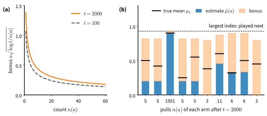
The size of the bonus comes from Hoeffding’s inequality (Hoeffding 1963): the mean \(\hat\mu_n\) of \(n\) independent rewards in \([0, 1]\) exceeds the true mean \(\mu\) by more than \(h\) with probability at most \(e^{-2 n h^2}\), and likewise falls below it. With \(h = \kappa \sqrt{\log t / n}\), the true mean lies above the index with probability at most \(t^{-2\kappa^2}\), for a fixed count \(n\). A larger \(\kappa\) makes such failures rarer and spends more pulls on bad arms. With \(\kappa = \sqrt{2}\) the rule is UCB1 of Auer et al. (2002), whose regret grows logarithmically in \(t\) on every bandit with rewards in \([0, 1]\); the same holds for every \(\kappa > 1\) (Bubeck and Cesa-Bianchi 2012), and exercise 2 derives the bound.
14.4.2.2 Thompson Sampling
Thompson’s rule of 1933 replaces the bonus by a belief. It keeps, for each arm, a posterior distribution over the arm’s mean, draws one sample from each posterior, and pulls the arm with the largest draw. For rewards in \(\{0, 1\}\) and a uniform prior on \([0, 1]\), the posterior after \(w\) wins in \(n\) pulls is the Beta distribution \(\mathrm{Beta}(1 + w, 1 + n - w)\). An arm with \(3\) wins in \(4\) pulls has the posterior \(\mathrm{Beta}(4, 2)\), with mean \(2/3\) but wide. An untried arm has the uniform \(\mathrm{Beta}(1, 1)\), and its draw beats a draw from \(\mathrm{Beta}(4, 2)\) with probability \(1/3\). As pulls accumulate, the posteriors narrow, and each arm is pulled with the posterior probability that it is the best one. Thompson sampling also has logarithmic regret (Agrawal and Goyal 2012), and it has no constant to choose.
14.4.2.3 UCB and Thompson Sampling Compared
The function ucb(kappa) returns the UCB rule with coefficient \(\kappa\), and thompson draws from the Beta posteriors. We run UCB with \(\kappa = 0.5\), a value chosen for these arms that we examine below, and Thompson sampling, and then plot all five rules. d2l.plot_curves draws the median over the runs with the band between the quartiles, here at 100 pulls spaced evenly on logarithmic axes:
def ucb(kappa):
    """The UCB rule with coefficient kappa: each arm once, then the largest
    index mean + kappa * sqrt(log t / n)."""
    def rule(wins, count, t, rng):
        if (count == 0).any():          # play each arm once before pricing any
            return int(np.argmax(count == 0))
        bonus = kappa * np.sqrt(np.log(t) / count)
        return int(np.argmax(wins / count + bonus))
    return rule

def thompson(wins, count, t, rng):
    """Draw each arm's mean from its Beta posterior; play the largest draw."""
    return int(rng.beta(1 + wins, 1 + count - wins).argmax())

for i, (name, rule) in enumerate([('UCB, kappa = 0.5', ucb(0.5)),
                                  ('Thompson', thompson)], 3):
    regret[name] = regret_runs(arms, rule, i)
    report(name, regret[name])
pulls = np.unique(np.geomspace(1, 2000, 100).astype(int))  # even on a log axis
d2l.plot_curves({name: r[:, pulls - 1] for name, r in regret.items()},
                xlabel='pulls', ylabel='cumulative regret', x=pulls,
                xscale='log', yscale='log', band='iqr')
UCB, kappa = 0.5: regret after 2000 pulls: median 39 (quartiles 29 to 40)
Thompson: regret after 2000 pulls: median 30 (quartiles 26 to 36)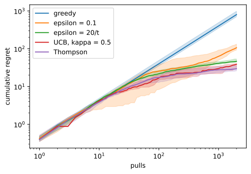
def ucb(kappa):
    """The UCB rule with coefficient kappa: each arm once, then the largest
    index mean + kappa * sqrt(log t / n)."""
    def rule(wins, count, t, rng):
        if (count == 0).any():          # play each arm once before pricing any
            return int(np.argmax(count == 0))
        bonus = kappa * np.sqrt(np.log(t) / count)
        return int(np.argmax(wins / count + bonus))
    return rule

def thompson(wins, count, t, rng):
    """Draw each arm's mean from its Beta posterior; play the largest draw."""
    return int(rng.beta(1 + wins, 1 + count - wins).argmax())

for i, (name, rule) in enumerate([('UCB, kappa = 0.5', ucb(0.5)),
                                  ('Thompson', thompson)], 3):
    regret[name] = regret_runs(arms, rule, i)
    report(name, regret[name])
pulls = np.unique(np.geomspace(1, 2000, 100).astype(int))  # even on a log axis
d2l.plot_curves({name: r[:, pulls - 1] for name, r in regret.items()},
                xlabel='pulls', ylabel='cumulative regret', x=pulls,
                xscale='log', yscale='log', band='iqr')
UCB, kappa = 0.5: regret after 2000 pulls: median 39 (quartiles 29 to 40)
Thompson: regret after 2000 pulls: median 30 (quartiles 26 to 36)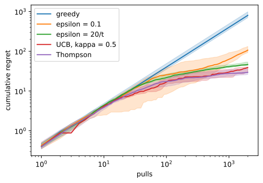
Both rules end with a median regret of roughly \(30\) to \(40\), about a third of the fixed \(\epsilon\) and below the annealed rule. They are close to each other: the difference between them is smaller than the spread over runs. On logarithmic axes a regret that grows linearly is a line of slope one. Greedy and fixed \(\epsilon\) approach that slope, while UCB, Thompson sampling and the annealed rule bend away from it. \(2000\) pulls cannot establish an asymptotic rate, but the bend is what logarithmic growth looks like.
14.4.2.4 The UCB Coefficient
The value \(\kappa = 0.5\) lies below the range \(\kappa > 1\) that the theory covers. How much does the coefficient matter? The cell plays forty runs for each of three coefficients and prints the median and extremes of the regret:
for j, kappa in enumerate([0.15, 0.5, np.sqrt(2)]):
    r = regret_runs(arms, ucb(kappa), 10 + j, num_runs=40)[:, -1]
    print(f'kappa = {kappa:.2f}: regret after 2000 pulls over 40 runs: median '
          f'{np.median(r):3.0f}, min {r.min():3.0f}, max {r.max():3.0f}')
kappa = 0.15: regret after 2000 pulls over 40 runs: median 8, min 4, max 709
kappa = 0.50: regret after 2000 pulls over 40 runs: median 37, min 20, max 50
kappa = 1.41: regret after 2000 pulls over 40 runs: median 205, min 170, max 245for j, kappa in enumerate([0.15, 0.5, np.sqrt(2)]):
r = regret_runs(arms, ucb(kappa), 10 + j, num_runs=40)[:, -1]
print(f'kappa = {kappa:.2f}: regret after 2000 pulls over 40 runs: median '
f'{np.median(r):3.0f}, min {r.min():3.0f}, max {r.max():3.0f}')kappa = 0.15: regret after 2000 pulls over 40 runs: median 8, min 4, max 709
kappa = 0.50: regret after 2000 pulls over 40 runs: median 37, min 20, max 50
kappa = 1.41: regret after 2000 pulls over 40 runs: median 205, min 170, max 245At \(2000\) pulls the coefficient decides the result. UCB1, \(\kappa = \sqrt{2}\), ends near \(200\), five to six times the regret of \(\kappa = 0.5\). With \(\kappa = 0.15\) the median is the smallest, about ten, but the maximum is large. With so small a bonus, a run in which the best arm starts with a few unlucky pulls can settle on a worse arm and keep losing \(0.3\) or more per pull. This happens in roughly one run in ten; the median hides these runs, and the mean does not.
One might expect the theory’s \(\kappa\) to win once the horizon is long enough. On these arms it does not: in runs of \(10^5\) pulls and more, which exercise 4 reproduces, \(\kappa = \sqrt{2}\) keeps six to eight times the regret of \(\kappa = 0.5\), and both grow like \(\log t\). The bonus accounts for the factor. UCB keeps pulling a worse arm \(a\) until its bonus \(\kappa\sqrt{\log t / n(a)}\) has shrunk to about \(\Delta_a\), that is for about \(\kappa^2 \log t / \Delta_a^2\) pulls, so in long runs the ratio of the two regrets approaches \((\sqrt{2}/0.5)^2 = 8\). What the theory guarantees is something else: \(\kappa = \sqrt{2}\) has logarithmic regret on every bandit with rewards in \([0, 1]\), and \(\kappa = 0.5\) has no such guarantee. Hoeffding’s inequality must hold for the worst case, an arm with variance \(1/4\). The best arm here has variance \(0.9 \times 0.1 = 0.09\), so its empirical mean is more accurate than the inequality assumes, and a smaller bonus is enough on this problem. Thompson sampling matches the tuned UCB rule without a constant to tune.
14.4.2.5 A Lower Bound on Regret
How low can regret go? Lai and Robbins proved that any rule that does well on every bandit of a family must, in \(t\) pulls, pull each worse arm \(a\) at least about \(\ln t / D(\mu_a \,\|\, \mu^*)\) times (Lai and Robbins 1985). Here
\[D(p \,\|\, q) = p \ln \frac{p}{q} + (1 - p) \ln \frac{1 - p}{1 - q}\]
is the relative entropy between Bernoulli distributions with means \(p\) and \(q\). It is small when the two means are close, so an arm that is nearly as good as the best is hard to tell apart and must be pulled more often. For the arm with mean \(0.60\), \(D(0.60 \,\|\, 0.90) = 0.31\), and it must be pulled about \(\ln 2000 / 0.31 \approx 24\) times by round \(2000\). With Equation 14.4.1, the regret of every such rule grows at least like \(\ln t\). UCB and Thompson sampling grow at this rate, so in long runs no rule does better by more than a constant factor; fixed \(\epsilon\), whose regret grows linearly, does not reach this rate.
14.4.3 Exploration in MDPs
In a bandit every arm can be pulled in every round. In an MDP, a state-action pair can be tried only from its state, and reaching that state may take a particular sequence of actions. Random actions produce a given sequence with a probability that falls geometrically in its length: with two actions, a particular sequence of \(k\) actions comes up with probability \(2^{-k}\).
14.4.3.1 A Chain of States
A chain makes this exact. It has \(N\) states in a row and starts in state \(0\). Action \(1\) moves one state on, action \(0\) returns to the start, and entering the last state gives reward \(1\) and ends the episode, which is cut after \(2N\) steps. To succeed, the agent must choose action \(1\) in \(N - 1\) consecutive steps. The function chain builds this MDP as a d2l.TabularMDP(P, r, gamma), the arrays of Section 14.1: P[s, a] is the distribution of the next state and r[s, a] the expected reward. The function success_random computes the exact probability that uniformly random actions reach the end within horizon steps. It averages the kernel over the two actions, \(P_\pi(s' \mid s) = \frac12 \sum_a P(s' \mid s, a)\), and propagates the state distribution from state \(0\) through \(P_\pi\) one step at a time. The last state is absorbing, so its probability after horizon steps is the probability of having arrived:
def chain(N, gamma):
    """N states in a row: action 1 moves one state on, action 0 returns to
    the start; entering the last state pays 1 and ends the episode."""
    P, r = np.zeros((N, 2, N)), np.zeros((N, 2))
    P[:, 0, 0] = 1
    P[np.arange(N - 1), 1, np.arange(1, N)] = 1
    P[N - 1] = 0
    P[N - 1, :, N - 1] = 1              # the last state is absorbing
    r[N - 2, 1] = 1
    return d2l.TabularMDP(P, r, gamma)

def success_random(mdp, horizon):
    """Exact probability that uniformly random actions, started in state 0,
    reach the last state within `horizon` steps."""
    P_pi, d = mdp.P.mean(axis=1), np.eye(mdp.num_states)[0]
    for _ in range(horizon):
        d = d @ P_pi
    return d[-1]
def chain(N, gamma):
"""N states in a row: action 1 moves one state on, action 0 returns to
the start; entering the last state pays 1 and ends the episode."""
P, r = np.zeros((N, 2, N)), np.zeros((N, 2))
P[:, 0, 0] = 1
P[np.arange(N - 1), 1, np.arange(1, N)] = 1
P[N - 1] = 0
P[N - 1, :, N - 1] = 1 # the last state is absorbing
r[N - 2, 1] = 1
return d2l.TabularMDP(P, r, gamma)
def success_random(mdp, horizon):
"""Exact probability that uniformly random actions, started in state 0,
reach the last state within `horizon` steps."""
P_pi, d = mdp.P.mean(axis=1), np.eye(mdp.num_states)[0]
for _ in range(horizon):
d = d @ P_pi
return d[-1]d2l.q_learning(seed, Q, visits, env, num_episodes, gamma, alpha, epsilon) of Section 14.3 updates the table Q in place from transitions it collects with \(\epsilon\)-greedy actions, counts visits in visits, and yields the return of each episode. It touches the environment only through env.reset and env.step, and the class ModelEnv gives a TabularMDP these two methods: reset puts the agent in state \(0\), and step draws the next state from P[s, a], reporting termination in a terminal state and truncation after max_steps steps.
The learner is the Q-learning of Section 14.3 with one change: every entry of the table starts at \(1\), an upper bound on every return, and the agent acts greedily, \(\epsilon = 0\). This is optimistic initialization, the idea behind UCB applied to a table: an untried pair looks as good as anything can be. For comparison, the cell prints the expected number of episodes until random actions first succeed, the inverse of the probability from success_random. Q-learning from a zero table acts exactly like this until its first success, whatever its \(\epsilon\), because every row is a tie broken at random (exercise 1):
class ModelEnv:
    """Gymnasium's reset/step on a TabularMDP: start in state 0, draw s'
    from P[s, a], end in a terminal state or after max_steps steps."""
    def __init__(self, mdp, terminal, max_steps):
        self.mdp, self.terminal, self.max_steps = mdp, terminal, max_steps
        self.rng = np.random.default_rng(0)

    def reset(self, seed=None):
        if seed is not None:
            self.rng = np.random.default_rng(seed)
        self.s, self.t = 0, 0
        return self.s, {}

    def step(self, a):
        s, self.t = self.s, self.t + 1
        self.s = int(self.rng.choice(self.mdp.num_states, p=self.mdp.P[s, a]))
        return (self.s, self.mdp.r[s, a], self.s in self.terminal,
                self.t >= self.max_steps, {})

for N in (4, 8, 12, 16, 20):
    mdp = chain(N, gamma=0.95)
    env = ModelEnv(mdp, terminal={N - 1}, max_steps=2 * N)
    first = []
    for seed in range(20):
        Q = np.ones((N, 2))             # optimistic: 1 bounds every return
        for k, ret in enumerate(d2l.q_learning(
                seed, Q, np.zeros_like(Q), env, 100, mdp.gamma,
                epsilon=lambda episode: 0.0)):
            if ret > 0:
                break
        first.append(k + 1)
    print(f'N = {N:2d}: episodes to the first success: random '
          f'{1 / success_random(mdp, 2 * N):5.0f} (mean), optimistic '
          f'{np.median(first):2.0f} (median, max {max(first)})')
N = 4: episodes to the first success: random 2 (mean), optimistic 2 (median, max 2)
N = 8: episodes to the first success: random 23 (mean), optimistic 3 (median, max 4)
N = 12: episodes to the first success: random 273 (mean), optimistic 4 (median, max 5)
N = 16: episodes to the first success: random 3449 (mean), optimistic 6 (median, max 7)
N = 20: episodes to the first success: random 45590 (mean), optimistic 8 (median, max 10)class ModelEnv:
"""Gymnasium's reset/step on a TabularMDP: start in state 0, draw s'
from P[s, a], end in a terminal state or after max_steps steps."""
def __init__(self, mdp, terminal, max_steps):
self.mdp, self.terminal, self.max_steps = mdp, terminal, max_steps
self.rng = np.random.default_rng(0)
def reset(self, seed=None):
if seed is not None:
self.rng = np.random.default_rng(seed)
self.s, self.t = 0, 0
return self.s, {}
def step(self, a):
s, self.t = self.s, self.t + 1
self.s = int(self.rng.choice(self.mdp.num_states, p=self.mdp.P[s, a]))
return (self.s, self.mdp.r[s, a], self.s in self.terminal,
self.t >= self.max_steps, {})
for N in (4, 8, 12, 16, 20):
mdp = chain(N, gamma=0.95)
env = ModelEnv(mdp, terminal={N - 1}, max_steps=2 * N)
first = []
for seed in range(20):
Q = np.ones((N, 2)) # optimistic: 1 bounds every return
for k, ret in enumerate(d2l.q_learning(
seed, Q, np.zeros_like(Q), env, 100, mdp.gamma,
epsilon=lambda episode: 0.0)):
if ret > 0:
break
first.append(k + 1)
print(f'N = {N:2d}: episodes to the first success: random '
f'{1 / success_random(mdp, 2 * N):5.0f} (mean), optimistic '
f'{np.median(first):2.0f} (median, max {max(first)})')N = 4: episodes to the first success: random 2 (mean), optimistic 2 (median, max 2)
N = 8: episodes to the first success: random 23 (mean), optimistic 3 (median, max 4)
N = 12: episodes to the first success: random 273 (mean), optimistic 4 (median, max 5)
N = 16: episodes to the first success: random 3449 (mean), optimistic 6 (median, max 7)
N = 20: episodes to the first success: random 45590 (mean), optimistic 8 (median, max 10)Random actions need about twice as many episodes for every state added: \(23\) at \(N = 8\), about \(3{,}400\) at \(N = 16\), about \(46{,}000\) at \(N = 20\). The optimistic learner needs a handful, about eight at \(N = 20\), a number that grows roughly in proportion to \(N\). Optimism works because a tried pair is marked as tried. After one try of a pair that pays nothing, its entry moves toward a target \(r + \gamma \max_{a'} Q(s', a')\) of at most \(\gamma < 1\), so it falls below every untried entry, which still reads \(1\). The greedy rule therefore prefers a pair it has not tried, and the learner works through the chain systematically instead of by chance. The number of episodes grows polynomially in \(N\) instead of exponentially.
14.4.3.2 Count-Based Bonuses
Optimistic initialization explores a pair until its first try lowers its value. In a stochastic MDP one try says little, and a pair needs repeated visits before its value is known. Count-based bonuses carry the UCB rule over to MDPs. They add to the reward of each pair a bonus that shrinks like \(1/\sqrt{n(s, a)}\) with its visit count, and let the value backups carry the bonus back to the states that lead there, so the agent plans its way toward pairs it knows little about. Model-based interval estimation does this with a learned model (Strehl and Littman 2008), and Q-learning with such bonuses has a regret that grows like the square root of the number of steps, up to factors polynomial in the size of the MDP (Jin et al. 2018). With a network in place of a table, states are rarely visited twice, and practical agents replace the count by a learned measure of novelty, such as the error of a network trained to predict a fixed random function of the state (Burda et al. 2019).
14.4.3.3 Coverage on the Lake
Does the lake need any of this? In Section 14.3, Q-learning on the calm lake, where every move goes where it is commanded, used the step size \(\alpha = 0.9\) for \(256\) episodes, and its greedy table solved the lake. We repeat that run under three schedules: greedy, \(\epsilon = 0\); always random, \(\epsilon = 1\); and the default of q_learning, d2l.linear_schedule(1.0, 0.05, 128), which lowers \(\epsilon\) linearly from \(1\) to \(0.05\) over the first half of training. In each of twenty runs the cell records, after every episode, the fraction of the \(44\) pairs tried at least once (\(11\) cells to act from, four actions each). It also records the fraction of training episodes that reach the goal, and whether the greedy policy of the final table does, which d2l.evaluate of Section 14.2 checks in one episode on this deterministic lake:
calm = gym.make('FrozenLake-v1', is_slippery=False)
live = np.array([c not in b'HG' for c in calm.unwrapped.desc.flatten()])
schedules = {'greedy': lambda k: 0.0,
             'epsilon = 1': lambda k: 1.0,
             'linear, 1 to 0.05': d2l.linear_schedule(1.0, 0.05, 128)}
coverage = {}
for name, epsilon in schedules.items():
    tried, won, solved = [], [], []
    for seed in range(20):
        Q, visits = np.zeros((16, 4)), np.zeros((16, 4))
        rets = []
        for ret in d2l.q_learning(seed, Q, visits, calm, 256, 0.95,
                                  alpha=lambda n: 0.9, epsilon=epsilon):
            rets.append(ret)
            tried.append((visits[live] > 0).mean())
        won.append(np.mean(rets))
        solved.append(d2l.evaluate(calm, lambda s, rng: int(Q[s].argmax()), 1))
    coverage[name] = np.array(tried).reshape(20, 256)
    print(f'{name:>17}: pairs tried {np.median(coverage[name][:, -1]):.0%}, '
          f'episodes won {np.median(won):.0%} (medians); greedy policy '
          f'solves {np.sum(solved):.0f}/20')
d2l.plot_curves(coverage, xlabel='episode', ylabel='fraction of pairs tried',
                band='iqr')
greedy: pairs tried 93%, episodes won 60% (medians); greedy policy solves 19/20
epsilon = 1: pairs tried 100%, episodes won 2% (medians); greedy policy solves 19/20
linear, 1 to 0.05: pairs tried 98%, episodes won 58% (medians); greedy policy solves 19/20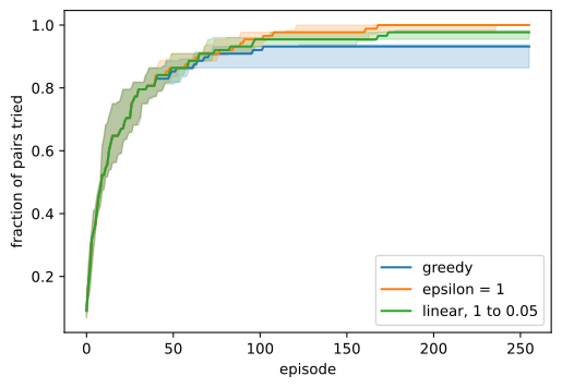
calm = gym.make('FrozenLake-v1', is_slippery=False)
live = np.array([c not in b'HG' for c in calm.unwrapped.desc.flatten()])
schedules = {'greedy': lambda k: 0.0,
             'epsilon = 1': lambda k: 1.0,
             'linear, 1 to 0.05': d2l.linear_schedule(1.0, 0.05, 128)}
coverage = {}
for name, epsilon in schedules.items():
    tried, won, solved = [], [], []
    for seed in range(20):
        Q, visits = np.zeros((16, 4)), np.zeros((16, 4))
        rets = []
        for ret in d2l.q_learning(seed, Q, visits, calm, 256, 0.95,
                                  alpha=lambda n: 0.9, epsilon=epsilon):
            rets.append(ret)
            tried.append((visits[live] > 0).mean())
        won.append(np.mean(rets))
        solved.append(d2l.evaluate(calm, lambda s, rng: int(Q[s].argmax()), 1))
    coverage[name] = np.array(tried).reshape(20, 256)
    print(f'{name:>17}: pairs tried {np.median(coverage[name][:, -1]):.0%}, '
          f'episodes won {np.median(won):.0%} (medians); greedy policy '
          f'solves {np.sum(solved):.0f}/20')
d2l.plot_curves(coverage, xlabel='episode', ylabel='fraction of pairs tried',
                band='iqr')
greedy: pairs tried 93%, episodes won 60% (medians); greedy policy solves 19/20
epsilon = 1: pairs tried 100%, episodes won 2% (medians); greedy policy solves 19/20
linear, 1 to 0.05: pairs tried 98%, episodes won 58% (medians); greedy policy solves 19/20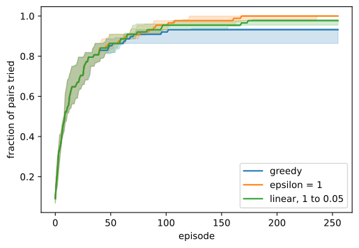
On the calm lake, random tie-breaking alone makes the greedy rule explore: it tries about nine pairs in ten, and its final greedy table solves the lake in nearly every run, as do the tables of the other two schedules. With \(\epsilon = 1\) the agent tries every pair but reaches the goal in almost none of its training episodes. Learning a good table and collecting reward while learning are different goals, and \(\epsilon\) trades one for the other. What limits all three schedules is the first success. Until then every entry is zero and every schedule acts at random, so for a given seed the first success arrives in the same episode under every schedule. The goal is six moves from the start, and random walks find it within a few dozen episodes. The lake is too small to show the difficulty of the chain. On slippery ice, the lake of this section’s opening, a single visit to a pair says little about it, and trying every pair once is not enough (exercise 1).
14.4.4 Exploration on the Verifier Task
The verifier task of Section 14.1 has four arithmetic prompts \(x\), nine candidate responses \(y\) shared by all of them, and a verifier with \(r(x, y) = 1\) if \(y\) is the prompt’s answer and \(0\) otherwise. The reference policy \(\pi_{\textrm{ref}}\), a softmax over one row of preferences per prompt, spreads its probability evenly over the eight ordinary candidates. It gives almost none to the ninth, a hedge that lists every answer and that the exact-match verifier never accepts. Two prompts, \(2+2\) and \(3 \times 4\), have their answer among the candidates; for \(8 \times 8\) and \(9 \times 9\) no candidate matches. A sampled response is correct with probability \(0.062\) on average over the prompts.
Each round a prompt arrives, one response is scored, and the episode ends. The prompt is a context that the agent observes but cannot influence, and the response is the arm. A bandit whose best arm depends on an observed context is a contextual bandit: the agent faces one bandit per prompt and, with a model, can share what it learns across prompts.
A language model explores such a task differently from the rules above. A common way to train it, derived in Section 14.7, samples a group of \(K\) responses to a prompt from the current policy, scores them, and raises the probability of the responses that scored above the group’s average while lowering those below it. A group in which every response scores the same has nothing above or below its average and changes nothing. If the policy answers a prompt correctly with probability \(p = \pi(\textrm{correct} \mid x)\), a group of \(K\) independent responses is identical with probability
\[(1 - p)^K + p^K, \tag{14.4.3}\]
the chance that all \(K\) are wrong plus the chance that all are right. The cell samples \(1{,}000\) groups per prompt and compares the fraction of identical groups with this formula. It does so at the reference policy and at a policy that has nearly solved the two answerable prompts, built by hand by raising the preference of each correct answer by \(5\); it is not a trained policy. The array R[x, y] holds the verifier’s score of every pair:
task = d2l.VerifierTask()
R = np.array([[task.verify(x, y) for y in range(len(task.resp))]
              for x in range(len(task.prompts))])
rng = np.random.default_rng(0)
for name, pi in [('reference', task.pi_ref),
                 ('solved', task.policy(task.theta_ref + 5 * R))]:
    p = (pi * R).sum(axis=1)            # chance that one response is right
    for K in (2, 8, 32):
        same = []                       # per prompt: all K rewards equal
        for x in range(len(task.prompts)):
            ys = rng.choice(len(task.resp), (1000, K), p=pi[x])
            same.append((R[x, ys] == R[x, ys[:, :1]]).all(axis=1).mean())
        print(f'{name:>9}, K = {K:2d}: identical {np.round(same, 2)}, '
              f'mean {np.mean(same):.2f}, '
              f'exact {np.mean((1 - p) ** K + p ** K):.2f}')
reference, K = 2: identical [0.78 0.78 1. 1. ], mean 0.89, exact 0.89
reference, K = 8: identical [0.35 0.33 1. 1. ], mean 0.67, exact 0.67
reference, K = 32: identical [0.01 0.02 1. 1. ], mean 0.51, exact 0.51
solved, K = 2: identical [0.89 0.93 1. 1. ], mean 0.96, exact 0.96
solved, K = 8: identical [0.67 0.7 1. 1. ], mean 0.84, exact 0.85
solved, K = 32: identical [0.21 0.21 1. 1. ], mean 0.60, exact 0.61task = d2l.VerifierTask()
R = np.array([[task.verify(x, y) for y in range(len(task.resp))]
for x in range(len(task.prompts))])
rng = np.random.default_rng(0)
for name, pi in [('reference', task.pi_ref),
('solved', task.policy(task.theta_ref + 5 * R))]:
p = (pi * R).sum(axis=1) # chance that one response is right
for K in (2, 8, 32):
same = [] # per prompt: all K rewards equal
for x in range(len(task.prompts)):
ys = rng.choice(len(task.resp), (1000, K), p=pi[x])
same.append((R[x, ys] == R[x, ys[:, :1]]).all(axis=1).mean())
print(f'{name:>9}, K = {K:2d}: identical {np.round(same, 2)}, '
f'mean {np.mean(same):.2f}, '
f'exact {np.mean((1 - p) ** K + p ** K):.2f}')reference, K = 2: identical [0.78 0.78 1. 1. ], mean 0.89, exact 0.89
reference, K = 8: identical [0.35 0.33 1. 1. ], mean 0.67, exact 0.67
reference, K = 32: identical [0.01 0.02 1. 1. ], mean 0.51, exact 0.51
solved, K = 2: identical [0.89 0.93 1. 1. ], mean 0.96, exact 0.96
solved, K = 8: identical [0.67 0.7 1. 1. ], mean 0.84, exact 0.85
solved, K = 32: identical [0.21 0.21 1. 1. ], mean 0.60, exact 0.61The sampled fractions agree with the formula. Half of all groups are identical at every \(K\): on the two prompts without a correct candidate every response fails, and no amount of sampling finds an answer that the policy cannot produce. On the two answerable prompts the reference is right with probability \(p \approx 0.125\), and larger groups are more often mixed: about \(78\%\) of the groups of two are identical, a third of the groups of eight, and almost none of the groups of \(32\). Once a prompt is nearly solved, groups become identical again, about two thirds of them at \(K = 8\), now because almost every response is right, and learning on that prompt slows.
The learner explores only through its own sampling. The probability that a group contains at least one correct response, \(1 - (1 - p)^K\), is the pass@\(K\) score used to evaluate models for code and reasoning (Chen et al. 2021). On a prompt that the policy usually fails, it is nearly the probability that a group can teach anything. Sampling at a higher temperature spreads probability over more responses and mixes more groups on a prompt the policy has nearly solved, at the cost of more wrong answers. It cannot help where no candidate is right.
Every rule in this section learns which actions are good by trying them, and the trying costs pulls of worse arms, episodes of random walking, or groups that teach nothing. On the chain an untried pair is hard to reach, and on the verifier task a correct answer that the policy never produces is never found. An expert who shows good actions would spare the agent all of this, and Section 14.5 learns from such demonstrations.
14.4.5 Summary
An agent that learns from its own actions must try actions that look worse to find out whether they are, and regret measures what this costs against an agent that knew the best action from the start. On a ten-armed bandit, the greedy rule settles on the first arm that pays out, and a fixed \(\epsilon\) loses the same amount per pull forever. An \(\epsilon\) that decays like \(1/t\), UCB and Thompson sampling make regret grow only like the logarithm of the number of pulls, which Lai and Robbins showed is the best possible rate. UCB’s coefficient decides its regret on a given problem: the coefficient of the theory is safe on every bandit and slower on this one. In an MDP, random actions find a required sequence of actions with a probability that falls geometrically in its length, while optimistic values make the agent seek out untried pairs. When a verifier scores groups of sampled responses, groups that score alike carry no signal, and the policy’s own sampling is its only exploration.
14.4.6 Exercises
[code] The exploration schedule. ●● On a zero-initialized table,
epsilon_greedybreaks every tie uniformly at random, and every reward of FrozenLake is nonnegative.- Show that every entry of the table stays exactly zero until the first successful episode, and that until then every \(\epsilon\) produces the same behavior. What does this imply for the episode of the first success as a criterion for choosing \(\epsilon\)?
- After the first success, which entries are positive? Show that an entry, once positive, stays positive, and that the greedy rule, \(\epsilon = 0\), never again tries the zero entries of a row that contains a positive entry. The coverage experiment of this section shows this rule trying about nine pairs in ten on the calm lake and learning to succeed there. Predict whether it also learns a good policy on slippery ice.
- The optional argument
epsilonofq_learningis a function from the episode index to the exploration rate, such as those returned bylinear_schedule. On the slippery lake, with the \(4000\) episodes of Section 14.3, run five seeds each with \(\epsilon\) held at \(0\), \(0.1\), \(0.5\) and \(1\), and with the schedulelinear_schedule(1.0, 0.05, num_episodes // 2)thatq_learninguses in Section 14.3. For each setting, report the mean training return, the success rate of the final greedy policy underd2l.evaluateover \(1000\) episodes, the fraction of pairs tried, and \(\max_s |\max_a \hat{Q}(s, a) - V^*(s)|\). Was your prediction right? - Rank the settings by training return and by greedy success rate. Where do the two rankings disagree, and what explains the disagreement?
Logarithmic regret of UCB. ●● With \(\kappa = \sqrt{2}\), the rule Equation 14.4.2 is UCB1 of Auer et al. (2002), whose Theorem 1 bounds the expected regret after \(t\) pulls of arms with rewards in \([0, 1]\) by \[\sum_{a:\, \Delta_a > 0} \frac{8 \ln t}{\Delta_a} + \Big(1 + \frac{\pi^2}{3}\Big) \sum_a \Delta_a, \qquad \Delta_a = \mu^* - \mu_a. \tag{14.4.4}\] Derive this bound. The tool is Hoeffding’s inequality: the mean \(\hat{\mu}_n\) of \(n\) independent rewards in \([0, 1]\) with mean \(\mu\) satisfies \[P(\hat{\mu}_n \geq \mu + h) \leq e^{-2 n h^2}, \tag{14.4.5}\] and likewise for the lower tail.
- Fix a suboptimal arm \(a\) and let \(n_0 = \lceil 8 \ln t / \Delta_a^2 \rceil\). Show that if arm \(a\) is pulled at a step \(u \leq t\) while \(n(a) \geq n_0\), then either the index of the best arm lies at or below \(\mu^*\), or the empirical mean of arm \(a\) exceeds \(\mu_a\) by more than its bonus.
- For fixed pull counts of both arms, bound the probability of each of the two events at step \(u\) by \(u^{-4}\). Take a union bound over the counts and sum over \(u\) to show \(\mathbb{E}[n(a)] \leq n_0 + \pi^2/3\) after \(t\) pulls.
- Combine part (b) with the regret decomposition Equation 14.4.1 to obtain the theorem. Evaluate the bound for
armsat \(t = 2000\) and compare it with the median regret near \(200\) that the coefficient sweep of this section prints for \(\kappa = \sqrt{2}\). Which step of the proof loses the most? - Repeat the argument for a general coefficient \(\kappa\). For which \(\kappa\) does the sum over steps in part (b) still converge, and what does the answer say about the section’s choice \(\kappa = 0.5\)? (The union bound over counts is loose; a peeling argument of (Bubeck and Cesa-Bianchi 2012) reaches every \(\kappa > 1\).)
Thompson’s posterior. ● Thompson sampling draws each arm’s mean from \(\mathrm{Beta}(1 + w, 1 + n - w)\) after \(w\) wins in \(n\) pulls.
- Show that this is the posterior of a Bernoulli mean under the uniform prior on \([0, 1]\).
- Arm A has \(3\) wins in \(4\) pulls and arm B is untried. Show that Thompson sampling pulls B with probability \(1/3\). More generally, show that against an untried arm it pulls the untried one with probability one minus the posterior mean of the other.
- Show that, given the data, Thompson sampling pulls each arm with the posterior probability that this arm has the largest mean.
- [code] Replace the uniform prior by \(\mathrm{Beta}(1, 9)\), which expects arms to be bad, and by \(\mathrm{Beta}(9, 1)\), which expects them to be good. How does the median regret after \(2000\) pulls change? Which of the two priors acts like optimistic initialization, and why?
[code] Long horizons. ●●
bandit_runplays one run at a time.- Write a version that plays many runs at once: keep
winsandcountas arrays of shape (runs, arms) and choose the arms of all runs in one step, for UCB and for Thompson sampling. Check that its medians at \(2000\) pulls agree with those of this section up to the spread over runs. - Run \(200\) runs of UCB with \(\kappa \in \{0.15, 0.3, 0.5, \sqrt{2}\}\) and of Thompson sampling to \(10^5\) pulls, and plot the median regret on logarithmic axes. Does \(\kappa = \sqrt{2}\) catch up with \(\kappa = 0.5\)?
- For \(\kappa = 0.15\), plot the mean regret as well as the median. Why do they grow at different rates, and which of the two describes the risk to a user who runs the rule once?
- Write a version that plays many runs at once: keep
[extended] Deep exploration. ●● Take the chain of this section: states \(0, \ldots, N-1\), start in state \(0\), action \(0\) returns to state \(0\), action \(1\) advances one state, reaching state \(N-1\) gives reward \(1\) and terminates, and episodes are truncated after \(2N\) steps.
- Show that the uniformly random policy succeeds in one episode with probability at most \(2N \cdot 2^{-(N-1)}\), so that the expected number of episodes up to the first success is at least \(2^{N-2}/N\), and compare the bound with the exact values that the chain cell prints. By part (a) of exercise 1, \(\epsilon\)-greedy Q-learning from a zero table acts uniformly at random until its first success, so the bound holds for it whatever the value of \(\epsilon\).
- Trace the first episodes of the optimistic greedy learner on the chain with \(N = 4\): which entries does each episode lower? Use the pattern to argue that the number of episodes it needs grows at most polynomially in \(N\).
- Move both learners to
gym.make('FrozenLake-v1', map_name='8x8', is_slippery=True), which truncates at \(100\) steps. Compare the optimistic greedy learner with the zero-initialized learner under the schedulelinear_schedule(1.0, 0.05, num_episodes // 2)at \(4000\) and \(20000\) episodes, five seeds each. Report the success rate of the greedy policy underd2l.evaluate, the environment steps used, and, as a reference, the success rate of the optimal policy computed by value iteration. Does optimism keep its advantage on a stochastic map, and what does it cost?
The project takes a few minutes of CPU time.
Groups that teach nothing. ● On a prompt that the policy answers correctly with probability \(p\), a group of \(K\) independent responses is identical with probability \((1 - p)^K + p^K\).
- For a fixed \(K \geq 2\), which \(p\) makes a mixed group most likely, and how likely is it then?
- For small \(p\), show that the smallest \(K\) for which a group is mixed with probability at least \(1/2\) is about \(\ln 2 / p\). Evaluate it for the reference policy of the verifier task, \(p \approx 0.125\), and for \(p = 0.01\).
- The prompts of a training set have success probabilities \(p\) spread uniformly over \([0, 1]\). What fraction of the groups of size \(K = 8\) is identical, and which prompts produce them?
- On the two prompts of
VerifierTaskwithout a correct candidate, every group is identical for every \(K\) and every sampling temperature. Name two changes, to the task or to the learner, that would let it learn on these prompts, and say what each needs that the verifier alone does not provide.