from d2l import torch as d2l
import torch
from torch import nn
from torch.nn import functional as F7.8 Convolutional Network Design Spaces
Every architecture in this chapter was designed by hand. AlexNet (Section 7.1) established that deep networks beat feature engineering; VGG (Section 7.2.1) organized convolutions into repeated blocks of \(3 \times 3\) kernels; NiN (Section 7.2.2) mixed channels with \(1 \times 1\) convolutions and aggregated with global pooling; GoogLeNet (Section 7.2.3) combined branches of different convolution widths; ResNet (Section 7.4) rebiased networks towards the identity mapping, making great depth trainable; and ResNeXt (Section 7.4.5) added grouped convolutions for a better parameter–computation trade-off. This network engineering succeeded, but each step depended on the intuition of its designers rather than on any systematic exploration of the space of possible networks.
One alternative is neural architecture search (NAS) (Zoph and Le 2016; Liu et al. 2018): define a search space, then use reinforcement learning, evolutionary algorithms, or gradient-based relaxations to select an architecture by estimated performance. EfficientNet is a prominent result of this approach (Tan and Le 2019). NAS can require substantial computation, and a selected network does not by itself explain which design principles made it effective.
Radosavovic et al. (2020) propose instead to design the space from which networks are sampled. A distribution over architectures is parameterized so that typical samples perform well. This is cheaper than a large NAS procedure and exposes regularities shared by many architectures. The resulting constraints define the RegNetX and RegNetY families.
import tensorflow as tf
from d2l import tensorflow as d2l
from d2l import jax as d2l
from flax import nnx
import jaxfrom d2l import mxnet as d2l
from mxnet import np, npx, init
from mxnet.gluon import nn
npx.set_np()7.8.1 The AnyNet Design Space
Following Radosavovic et al. (2020), we first need a template for the family of networks to explore. A commonality of the designs in this chapter is that networks consist of a stem, a body, and a head. The stem performs initial image processing, often via convolutions with a larger window size. The body carries out the bulk of the transformation from raw images to object representations; it consists of multiple stages that operate on the image at decreasing resolutions, each stage built from one or more blocks. The head converts the result into the desired output, for instance via a softmax regressor for multiclass classification. This pattern is common to all networks from VGG to ResNeXt; for generic AnyNet networks, Radosavovic et al. (2020) used the ResNeXt block of Figure 7.4.5.
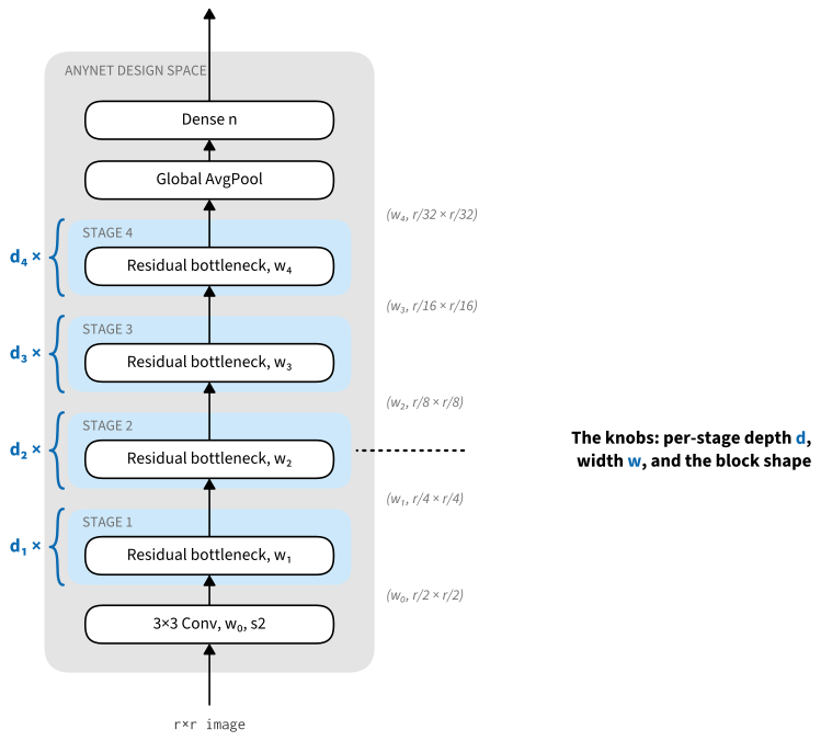
We now examine the structure of Figure 7.8.1. The stem takes RGB images (3 channels) and applies a \(3 \times 3\) convolution with a stride of \(2\), followed by batch norm, halving the resolution from \(r \times r\) to \(r/2 \times r/2\) and producing \(c_0\) channels that serve as input to the body.
Since the network is designed for ImageNet images of shape \(224 \times 224 \times 3\), the body reduces this to \(7 \times 7 \times c_4\) through 4 stages (recall that \(224 / 2^{1+4} = 7\)), each with an eventual stride of \(2\). The head is entirely standard: global average pooling, as in NiN (Section 7.2.2), followed by a fully connected layer emitting an \(n\)-dimensional vector for \(n\)-class classification.
Most of the design decisions live in the body. Each stage begins with a block that halves the resolution using a stride of \(2\) (the rightmost in Figure 7.8.1); to match shapes, its residual branch passes through a \(1 \times 1\) convolution. This block is followed by a variable number of ResNeXt blocks that leave both resolution and channel count unchanged. Each block may narrow its internal channels by a bottleneck ratio \(k_i \geq 1\), affording \(c_i/k_i\) channels inside the block for stage \(i\) (as the experiments will show, this is not really effective and should be skipped). Since we use ResNeXt blocks, we must also pick the number of groups \(g_i\) for grouped convolutions at stage \(i\).
This seemingly generic design space still leaves many parameters: block widths \(c_0, \ldots c_4\), depths per stage \(d_1, \ldots d_4\), bottleneck ratios \(k_1, \ldots k_4\), and numbers of groups \(g_1, \ldots g_4\), a total of 17 parameters and an unreasonably large number of configurations to explore. We will need tools to reduce this design space effectively. But first, let’s implement the generic design.
class AnyNet(d2l.Classifier):
    def stem(self, num_channels):
        return nn.Sequential(
            nn.LazyConv2d(num_channels, kernel_size=3, stride=2, padding=1),
            nn.LazyBatchNorm2d(), nn.ReLU())
class AnyNet(d2l.Classifier):
def stem(self, num_channels):
return tf.keras.models.Sequential([
tf.keras.layers.Conv2D(num_channels, kernel_size=3, strides=2,
padding='same'),
tf.keras.layers.BatchNormalization(),
tf.keras.layers.Activation('relu')])class AnyNet(d2l.Classifier):
def __init__(self, arch, stem_channels, lr=0.1, num_classes=10,
in_channels=1, rngs=None):
super().__init__()
self.save_hyperparameters(ignore=['rngs'])
rngs = nnx.Rngs(d2l.get_key()) if rngs is None else rngs
self.net = self.create_net(in_channels, rngs)
def stem(self, in_channels, num_channels, rngs):
return nnx.Sequential(
nnx.Conv(in_channels, num_channels, kernel_size=(3, 3),
strides=(2, 2), padding=(1, 1), rngs=rngs),
nnx.BatchNorm(num_channels, rngs=rngs), nnx.relu)class AnyNet(d2l.Classifier):
def stem(self, num_channels):
net = nn.Sequential()
net.add(nn.Conv2D(num_channels, kernel_size=3, padding=1, strides=2),
nn.BatchNorm(), nn.Activation('relu'))
return netEach stage consists of depth ResNeXt blocks, where num_channels specifies the block width. Note that the first block halves the height and width of input images.
@d2l.add_to_class(AnyNet)
def stage(self, depth, num_channels, groups, bot_mul):
    blk = []
    for i in range(depth):
        if i == 0:
            blk.append(d2l.ResNeXtBlock(num_channels, groups, bot_mul,
                use_1x1conv=True, strides=2))
        else:
            blk.append(d2l.ResNeXtBlock(num_channels, groups, bot_mul))
return nn.Sequential(*blk)@d2l.add_to_class(AnyNet)
def stage(self, depth, num_channels, groups, bot_mul):
net = tf.keras.models.Sequential()
for i in range(depth):
if i == 0:
net.add(d2l.ResNeXtBlock(num_channels, groups, bot_mul,
use_1x1conv=True, strides=2))
else:
net.add(d2l.ResNeXtBlock(num_channels, groups, bot_mul))
return net@d2l.add_to_class(AnyNet)
def stage(self, depth, num_channels, groups, bot_mul, in_channels, rngs):
blk = []
for i in range(depth):
if i == 0:
blk.append(d2l.ResNeXtBlock(num_channels, groups, bot_mul,
use_1x1conv=True, strides=(2, 2), in_channels=in_channels,
rngs=rngs))
else:
blk.append(d2l.ResNeXtBlock(num_channels, groups, bot_mul,
in_channels=num_channels, rngs=rngs))
return nnx.Sequential(*blk)@d2l.add_to_class(AnyNet)
def stage(self, depth, num_channels, groups, bot_mul):
net = nn.Sequential()
for i in range(depth):
if i == 0:
net.add(d2l.ResNeXtBlock(
num_channels, groups, bot_mul, use_1x1conv=True, strides=2))
else:
net.add(d2l.ResNeXtBlock(
num_channels, groups, bot_mul))
return netPutting the network stem, body, and head together, we complete the implementation of AnyNet.
@d2l.add_to_class(AnyNet)
def __init__(self, arch, stem_channels, lr=0.1, num_classes=10):
    super(AnyNet, self).__init__()
    self.save_hyperparameters()
    self.net = nn.Sequential(self.stem(stem_channels))
    for i, s in enumerate(arch):
        self.net.add_module(f'stage{i+1}', self.stage(*s))
    self.net.add_module('head', nn.Sequential(
        nn.AdaptiveAvgPool2d((1, 1)), nn.Flatten(),
        nn.LazyLinear(num_classes)))
self.net.apply(d2l.init_cnn)@d2l.add_to_class(AnyNet)
def __init__(self, arch, stem_channels, lr=0.1, num_classes=10):
super(AnyNet, self).__init__()
self.save_hyperparameters()
self.net = self.stem(stem_channels)
for i, s in enumerate(arch):
self.net.add(self.stage(*s))
self.net.add(tf.keras.models.Sequential([
tf.keras.layers.GlobalAvgPool2D(),
tf.keras.layers.Dense(units=num_classes)]))@d2l.add_to_class(AnyNet)
def create_net(self, in_channels, rngs):
layers = [self.stem(in_channels, self.stem_channels, rngs)]
stage_channels = self.stem_channels
for s in self.arch:
layers.append(self.stage(*s, stage_channels, rngs))
stage_channels = s[1]
layers.append(nnx.Sequential(
lambda x: x.mean(axis=(1, 2)), # global avg pooling over H, W (NHWC)
nnx.Linear(stage_channels, self.num_classes, rngs=rngs)))
return nnx.Sequential(*layers)@d2l.add_to_class(AnyNet)
def __init__(self, arch, stem_channels, lr=0.1, num_classes=10):
super(AnyNet, self).__init__()
self.save_hyperparameters()
self.net = nn.Sequential()
self.net.add(self.stem(stem_channels))
for i, s in enumerate(arch):
self.net.add(self.stage(*s))
self.net.add(nn.GlobalAvgPool2D(), nn.Dense(num_classes))
self.net.initialize(init.Xavier())7.8.2 Distributions and Parameters of Design Spaces
Parameters of a design space are hyperparameters of networks in that design space. Consider the problem of identifying good parameters in the AnyNet design space. We could try to find the single best parameter choice for a given amount of computation (e.g., FLOPs). But even with only two possible choices per parameter, we would have to explore \(2^{17} = 131072\) combinations. Moreover, exhaustive search provides little guidance about how to design a network: add a new stage type or operation and we start from scratch, and training stochasticity (rounding, shuffling) means no two runs produce exactly the same result anyway. A better strategy is to determine general guidelines for how parameter choices should be related, e.g., that the bottleneck ratio, the number of channels, blocks, and groups, or their change between stages, should be governed by a collection of simple rules. The approach in Radosavovic et al. (2019) relies on the following four assumptions:
- General design principles actually exist, so that many networks satisfying them offer good performance. Consequently, identifying a distribution over networks is a sensible strategy: there are many good needles in the haystack.
- We need not train networks to convergence to assess whether they are good; intermediate results are reliable guidance for final accuracy. Using such approximate proxies to optimize an objective is referred to as multi-fidelity optimization (Forrester et al. 2007). Design optimization is thus carried out based on the accuracy achieved after only a few passes through the dataset, reducing the cost significantly.
- Results obtained at a smaller scale (with fewer blocks and channels) generalize to larger ones, so optimization is carried out on structurally similar but smaller networks; only at the end do we verify that the resulting networks also perform well at scale.
- Aspects of the design can be approximately factorized, so that their effect on the outcome can be inferred somewhat independently.
These assumptions allow us to test many networks cheaply: we sample uniformly from the space of configurations and then judge a choice of design-space parameters by the distribution of errors it produces. Denote by \(F(e)\) the cumulative distribution function (CDF) for errors committed by networks of a given design space, drawn using probability distribution \(p\). That is,
\[F(e, p) \stackrel{\textrm{def}}{=} P_{\textrm{net} \sim p} \{e(\textrm{net}) \leq e\}. \tag{7.8.1}\]
Our goal is to find a distribution \(p\) over networks such that most networks have a very low error rate and the support of \(p\) is concise. Computing \(F\) exactly is infeasible, so we resort to a sample of networks \(\mathcal{Z} \stackrel{\textrm{def}}{=} \{\textrm{net}_1, \ldots \textrm{net}_n\}\) (with errors \(e_1, \ldots, e_n\), respectively) drawn from \(p\) and use the empirical CDF \(\hat{F}(e, \mathcal{Z})\) instead:
\[\hat{F}(e, \mathcal{Z}) = \frac{1}{n}\sum_{i=1}^n \mathbf{1}(e_i \leq e). \tag{7.8.2}\]
If the empirical CDF for one sampled design space lies above another, a larger fraction of its sampled networks achieve any given error threshold. This is an estimate of first-order stochastic dominance under the paper’s sampling and training protocol, not a universal ranking of architectures. Under that protocol, tying the bottleneck ratios \(k_i=k\) produces a CDF nearly indistinguishable from the original space (first panel of Figure 7.8.2). Tying the group widths, the number of channels per group, across stages has similarly little visible effect in the second panel. Together these constraints remove six parameters from the design space.

The next constraints require channels and depths to increase across stages: \(c_i\geq c_{i-1}\) and \(d_i\geq d_{i-1}\). In the third and fourth panels, these constrained spaces shift the sampled error CDF upward under the same protocol. The experiment supports retaining the constraints in this search space; it does not prove that every task or block family benefits from them.
7.8.3 RegNet
The resulting \(\textrm{AnyNetX}_E\) design space consists of simple networks following easy-to-interpret design principles:
- Share the bottleneck ratio \(k_i = k\) for all stages \(i\);
- Share the group width, the number of channels per group, across all stages;
- Increase network width across stages: \(c_{i} \leq c_{i+1}\);
- Increase network depth across stages: \(d_{i} \leq d_{i+1}\).
The RegNetX32 implementation below simplifies the second principle: it shares the number of groups across stages rather than the group width.
It remains to pick specific values for the parameters of the \(\textrm{AnyNetX}_E\) design space. Studying the best-performing networks from its distribution shows that network width ideally increases linearly with the block index \(j\) across the network, i.e., \(c_j \approx c_0 + c_a j\) with slope \(c_a > 0\); since block width can only change per stage, we arrive at a piecewise constant function engineered to match this dependence. Experiments also show that a bottleneck ratio of \(k = 1\) performs best, i.e., we are advised not to use bottlenecks at all.
We refer the interested reader to Radosavovic et al. (2020) for the design of specific networks at different amounts of computation. For instance, an effective 32-layer RegNetX variant is given by \(k = 1\) (no bottleneck), \(g = 16\) groups in every grouped convolution (group widths 2 and 5), with \(c_1 = 32\) and \(c_2 = 80\) channels for the first and second stage, respectively, chosen to be \(d_1=4\) and \(d_2=6\) blocks deep. These design principles continue to hold at larger scale, and they carry over to the Squeeze-and-Excitation variant (RegNetY) that adds a global channel activation (Hu et al. 2018), which we describe below.
class RegNetX32(AnyNet):
    def __init__(self, lr=0.1, num_classes=10):
        stem_channels, groups, bot_mul = 32, 16, 1
        depths, channels = (4, 6), (32, 80)
        super().__init__(
            ((depths[0], channels[0], groups, bot_mul),
             (depths[1], channels[1], groups, bot_mul)),
            stem_channels, lr, num_classes)
class RegNetX32(AnyNet):
def __init__(self, lr=0.1, num_classes=10):
stem_channels, groups, bot_mul = 32, 16, 1
depths, channels = (4, 6), (32, 80)
super().__init__(
((depths[0], channels[0], groups, bot_mul),
(depths[1], channels[1], groups, bot_mul)),
stem_channels, lr, num_classes)class RegNetX32(AnyNet):
def __init__(self, lr=0.1, num_classes=10, in_channels=1, rngs=None):
super().__init__(((4, 32, 16, 1), (6, 80, 16, 1)), 32,
lr, num_classes, in_channels, rngs)class RegNetX32(AnyNet):
def __init__(self, lr=0.1, num_classes=10):
stem_channels, groups, bot_mul = 32, 16, 1
depths, channels = (4, 6), (32, 80)
super().__init__(
((depths[0], channels[0], groups, bot_mul),
(depths[1], channels[1], groups, bot_mul)),
stem_channels, lr, num_classes)We can see that each RegNetX stage progressively reduces resolution and increases output channels.
RegNetX32().layer_summary((1, 1, 96, 96))Sequential output shape: torch.Size([1, 32, 48, 48])
Sequential output shape: torch.Size([1, 32, 24, 24])
Sequential output shape: torch.Size([1, 80, 12, 12])
Sequential output shape: torch.Size([1, 10])import logging
tf.get_logger().setLevel(logging.ERROR)
RegNetX32().layer_summary((1, 96, 96, 1))
tf.get_logger().setLevel(logging.WARNING)Conv2D output shape: (1, 48, 48, 32)
BatchNormalization output shape: (1, 48, 48, 32)
Activation output shape: (1, 48, 48, 32)
Sequential output shape: (1, 24, 24, 32)
Sequential output shape: (1, 12, 12, 80)
Sequential output shape: (1, 10)RegNetX32().layer_summary((1, 96, 96, 1))Sequential output shape: (1, 48, 48, 32)
Sequential output shape: (1, 24, 24, 32)
Sequential output shape: (1, 12, 12, 80)
Sequential output shape: (1, 10)RegNetX32().layer_summary((1, 1, 96, 96))Sequential output shape: (1, 32, 48, 48)
Sequential output shape: (1, 32, 24, 24)
Sequential output shape: (1, 80, 12, 12)
GlobalAvgPool2D output shape: (1, 80, 1, 1)
Dense output shape: (1, 10)7.8.3.1 Squeeze-and-Excitation Gates
The global channel activation that turns RegNetX into RegNetY is the squeeze-and-excitation (SE) gate (Hu et al. 2018). A convolution mixes information locally; an SE gate lets the network reweight entire channels based on global context. It squeezes each channel to a single number by global average pooling, passes the resulting vector of \(c\) channel summaries through a two-layer bottleneck MLP with a sigmoid output (the excitation), and multiplies each channel of the input by its gate value. The extra cost is negligible, about \(2c^2/r\) parameters for reduction ratio \(r\) and almost no FLOPs, since the MLP acts on a pooled vector rather than on the feature map. This is a simple form of attention, computed per channel rather than per location; the general mechanism is the subject of Chapter 10. The gate outlived its namesake network: EfficientNet (Tan and Le 2019) and most of the mobile architectures of Section 7.5 include SE blocks.
An SE gate is only a few lines: pool, two dense layers, rescale.
class SE(nn.Module):
    def __init__(self, num_channels, ratio=4):
        super().__init__()
        self.fc = nn.Sequential(
            nn.LazyLinear(num_channels // ratio), nn.ReLU(),
            nn.LazyLinear(num_channels), nn.Sigmoid())

    def forward(self, X):
        s = self.fc(X.mean(dim=(2, 3)))
        return X * s[:, :, None, None]

SE(32)(d2l.randn(2, 32, 16, 16)).shape
torch.Size([2, 32, 16, 16])class SE(tf.keras.Model):
def __init__(self, num_channels, ratio=4):
super().__init__()
self.fc = tf.keras.Sequential([
tf.keras.layers.Dense(num_channels // ratio, activation='relu'),
tf.keras.layers.Dense(num_channels, activation='sigmoid')])
def call(self, X):
s = self.fc(tf.reduce_mean(X, axis=(1, 2)))
return X * s[:, None, None, :]
SE(32)(tf.random.normal((2, 16, 16, 32))).shapeTensorShape([2, 16, 16, 32])class SE(nnx.Module):
def __init__(self, num_channels, ratio=4, rngs=None):
rngs = nnx.Rngs(d2l.get_key()) if rngs is None else rngs
self.squeeze = nnx.Linear(num_channels, num_channels // ratio,
rngs=rngs)
self.excite = nnx.Linear(num_channels // ratio, num_channels,
rngs=rngs)
def __call__(self, X):
s = X.mean(axis=(1, 2))
s = nnx.relu(self.squeeze(s))
s = nnx.sigmoid(self.excite(s))
return X * s[:, None, None, :]
X = jax.random.normal(d2l.get_key(), (2, 16, 16, 32))
SE(32)(X).shape(2, 16, 16, 32)class SE(nn.Block):
def __init__(self, num_channels, ratio=4):
super().__init__()
self.fc = nn.Sequential()
self.fc.add(nn.Dense(num_channels // ratio, activation='relu'),
nn.Dense(num_channels, activation='sigmoid'))
def forward(self, X):
s = self.fc(X.mean(axis=(2, 3)))
return X * s.reshape(s.shape + (1, 1))
se = SE(32)
se.initialize()
se(d2l.randn(2, 32, 16, 16)).shape(2, 32, 16, 16)The output has the same shape as the input: an SE gate can be dropped into any block, which is exactly how RegNetY, EfficientNet, and their successors use it.
7.8.4 Training
We train the 32-layer RegNetX on Fashion-MNIST as before.
model = RegNetX32(lr=0.05)
trainer = d2l.Trainer(max_epochs=10, num_gpus=1)
data = d2l.FashionMNIST(batch_size=128, resize=(96, 96))
trainer.fit(model, data)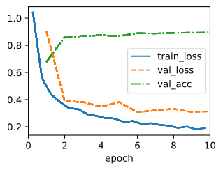
trainer = d2l.Trainer(max_epochs=10)
data = d2l.FashionMNIST(batch_size=128, resize=(96, 96))
with d2l.try_gpu():
    model = RegNetX32(lr=0.05)
    trainer.fit(model, data)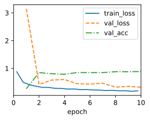
model = RegNetX32(lr=0.05)
trainer = d2l.Trainer(max_epochs=10, num_gpus=1)
data = d2l.FashionMNIST(batch_size=128, resize=(96, 96))
trainer.fit(model, data)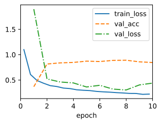
model = RegNetX32(lr=0.05)
trainer = d2l.Trainer(max_epochs=10, num_gpus=1)
data = d2l.FashionMNIST(batch_size=128, resize=(96, 96))
trainer.fit(model, data)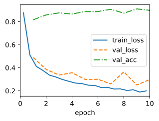
7.8.5 Comparing Convnets and Vision Transformers
For most of a decade, the networks in this chapter defined the state of the art in computer vision. Then came vision Transformers (Section 11.5) (Dosovitskiy et al. 2021; Touvron et al. 2021), which have far weaker inductive biases towards locality and translation equivariance (Section 6.1). They surpassed CNNs on large-scale image classification, and it became common to read that convolution was obsolete. The evidence that has accumulated since is more precise.
Controlled comparisons give a more qualified account of scaling. When convolutional networks receive modern training recipes and the same compute budget as vision Transformers, they can remain competitive: NFNets (Brock et al. 2021) match ViT accuracy at equal compute when pretrained at JFT-4B scale (Smith et al. 2023), and modernizing the recipe (Section 7.6) and architecture of a ResNet yields ConvNeXt (Section 7.7) (Liu et al. 2022), which is competitive with contemporary Transformers. The apparent gap between the two families around 2021 was mostly a gap in recipe and scale, not in representational power.
The two families now serve overlapping but distinct regimes. Transformers are common in foundation-scale pretraining and multimodal systems because they integrate with the tooling, scaling infrastructure, and language models built around the same architecture (Section 11.4.1). Convolutional networks remain effective for latency-constrained and edge deployment, small datasets, and many dense-prediction tasks. In medical image segmentation, the self-configuring convolutional U-Net nnU-Net performs strongly in controlled benchmarks (Isensee et al. 2021). And convolutions persist inside Transformers: Whisper, for example, feeds its Transformer encoder from a convolutional stem (Radford et al. 2023). Section 7.5 covers the deployment side of this division in detail.
The same pattern holds beyond classification. Diffusion image generators moved from convolutional U-Nets to diffusion Transformers at the frontier (Peebles and Xie 2023), while convolutional U-Nets remain standard in deployed and smaller systems.
The comparison suggests that locality and translation equivariance can improve data efficiency, while large-scale pretraining can let less constrained models learn useful spatial regularities. The balance depends on data, compute, latency, and task; neither architecture family dominates every regime. Chapter 11 develops the alternative architecture in full.
7.8.6 Summary
AnyNet turns architecture design into a distribution over block depths, widths, group widths, and bottleneck ratios. Under the RegNet sampling and training protocol, tying several stage parameters preserves the observed error distribution, while increasing widths and depths across stages improves it. RegNet further constrains stage widths to a quantized linear rule, producing a small, interpretable family rather than one selected network. These conclusions are empirical and depend on the block family, compute budget, and training recipe; the exercise below tests whether they survive a change to ConvNeXt blocks.
7.8.7 Exercises
- [code] Four stages at matched budget.
RegNetX32uses two stages. Extend it to the four stages of Figure 7.8.1, keeping widths and depths nondecreasing across stages and the parameter count within 10% ofRegNetX32. Compare validation accuracy and time per epoch on Fashion-MNIST at \(96 \times 96\). Work out the feature-map size at which each stage operates and explain what a \(3 \times 3\) convolution computes on the last one. - [code] ResNet blocks in RegNetX. Replace
d2l.ResNeXtBlockinAnyNet.stageby theResidualblock of Section 7.4, keeping the depths and widths ofRegNetX32. Compare parameter count, multiply-adds, and validation accuracy with the original. For a block that keeps its width \(c\), express the parameter count of both block types as a function of \(c\) and the number of groups \(g\), thegroupsargument ofd2l.ResNeXtBlock. Check both formulas against the parameters of one such block in each model. - [code] VioNet. ●
RegNetX32passesgroups=16, the number of groups, to stages of width 32 and 80, so its group widths, the channels per group, are 2 and 5. Build a baseline with the depths and widths ofRegNetX32and one group width of 16 shared by both stages. Then implement variants of the baseline that each violate one design principle of \(\textrm{AnyNetX}_E\) (Section 7.8.3) at roughly matched parameter count: widths that decrease across stages, depths that decrease across stages, group widths that differ between stages, and bottleneck ratios that differ between stages.- Report validation accuracy for each violation against the baseline.
- Which of depth \(d_i\), width \(c_i\), group width, and bottleneck ratio \(k_i\) matters most here?
- Compare your ranking with Figure 7.8.2. Which violations did the sampled design spaces of Radosavovic et al. (2020) also find harmless, and why does one network per violation give weaker evidence than an error CDF?
- Quantized linear widths. Radosavovic et al. (2020) turn the observation that width should grow linearly with the block index into a rule with three numbers. For \(d\) blocks, the target width of block \(j\) is \[u_j = w_0 + w_a\, j, \qquad j = 0, \ldots, d-1,\] the linear rule \(c_j \approx c_0 + c_a j\) of Section 7.8.3 with intercept \(w_0\) and slope \(w_a\). Each block is snapped to a geometric grid with ratio \(w_m\), \[s_j = \operatorname{round}\left(\frac{\log(u_j / w_0)}{\log w_m}\right), \qquad w_j = w_0\, w_m^{s_j}. \tag{7.8.3}\] Blocks with equal \(w_j\) form one stage.
- For \(d = 13\), \(w_0 = 24\), \(w_a = 36.44\), and \(w_m = 2.49\), compute the number of stages, the depth of each, and the stage widths rounded to the nearest multiple of 8. Compare with the RegNetX-200MF configuration in the paper.
- Describe how the number of stages, and how closely \(w_j\) tracks \(u_j\), change as \(w_m \to 1\) and as \(w_m\) grows large.
- A shared group width, the number of channels per group, must divide every stage width. Which of your widths violate this for a group width of 16, and how would you adjust them?
- [code] RegNetY. RegNetY adds the
SEgate of Section 7.8.3.1 to every block. InsertSEintod2l.ResNeXtBlockafter its grouped \(3 \times 3\) convolution, as Radosavovic et al. (2020) do, and build a RegNetY32 with the configuration ofRegNetX32.- Predict the added parameter count from the estimate of about \(2c^2/r\) per gate and verify it against the model.
- Compare validation accuracy and time per epoch with
RegNetX32. Where does the extra time come from, given that the gate adds almost no floating point operations? - Sweep the reduction ratio over \(r \in \{1, 4, 16\}\). How sensitive are accuracy and parameter count to \(r\)?
- [extended] Proxy reliability. ● The method of Section 7.8.2 assumes that accuracy after a few epochs predicts final accuracy and that results at small scale carry over to larger networks. Test both with eight configurations sampled from a two-stage AnyNet space with \(d_i \in \{2, 4, 6\}\), \(c_i \in \{16, 32, 64, 128\}\) subject to \(c_1 \le c_2\), a number of groups \(g \in \{4, 8\}\) shared by both stages (the
groupsargument ofd2l.ResNeXtBlock), and \(k = 1\). The rank correlation of two rankings is the correlation between the positions the networks occupy in them.- Train each configuration for 10 epochs on Fashion-MNIST at \(96 \times 96\), recording validation accuracy after every epoch. Compute the rank correlation between the ranking after 1, 2, and 5 epochs and the ranking after 10 epochs.
- Repeat the eight runs with every width halved and the input resized to \(48 \times 48\). Compute the rank correlation between the final rankings at small and at full scale.
- Which of the two assumptions holds up better in your experiment? What would a failure of the weaker one do to conclusions drawn from short, small-scale runs such as those behind Figure 7.8.2?
- Design spaces versus architecture search. Neural architecture search (Zoph and Le 2016; Liu et al. 2018) selects one network from a search space; the method of Section 7.8.2 constrains a distribution over networks.
- Explain why comparing empirical CDFs Equation 7.8.2 cannot identify the best network in a space, and why that is not its purpose.
- Of the four assumptions listed in Section 7.8.2, which does a NAS method that trains candidates briefly also rely on, and which are specific to the design-space approach?
- Name one failure mode of each approach: what can go wrong when a single architecture is selected by a proxy score, and what can go wrong when a design space is constrained by rules fitted to a sample?
- [extended] A ConvNeXt design space. ● The design spaces of Figure 7.8.2 were built from ResNeXt blocks. Build a two-stage AnyNet space from the
ConvNeXtBlockof Section 7.7 instead, with the stem and downsampling layer ofConvNeXt. Stage \(i\) has depth \(d_i \in \{1, 2, 4\}\), width \(c_i \in \{32, 64, 128\}\), and an expansion ratio in \(\{2, 4\}\).ConvNeXtBlockfixes the expansion ratio at 4, so add it as an argument.- Which of the AnyNet parameters \(d_i\), \(c_i\), \(g_i\), and \(k_i\) have a counterpart in this space, and which does the block fix?
- Sample 16 networks from the unconstrained space, 16 with one expansion ratio shared by both stages, and 16 with \(c_1 \le c_2\) and \(d_1 \le d_2\). Train each for two epochs on Fashion-MNIST at \(96 \times 96\) and plot the three empirical CDFs Equation 7.8.2. Which differences are resolved at 16 samples per space?
- Which of the RegNet design principles survive the change of block?