%matplotlib inline
from d2l import torch as d2l
import torch9.5 Momentum
Gradient descent uses only the gradient at the current point. On an ill-conditioned objective, a learning rate small enough for directions of high curvature gives slow progress in directions of low curvature. Momentum addresses this problem by maintaining a running average of past gradients, called the velocity. It requires one state buffer and a decay parameter, and is particularly effective on ill-conditioned objectives. The Adam family in Section 9.6 also incorporates momentum.
%matplotlib inline
from d2l import jax as d2l
import optax
9.5.1 An Ill-Conditioned Valley
In Section 9.2 we minimized \(f(\mathbf{x}) = x_1^2 + 2 x_2^2\), a moderately distorted bowl, and already saw the trajectory bend: the two coordinates wanted different step sizes. We make the distortion pronounced by flattening the first direction,
\[f(\mathbf{x}) = 0.1 x_1^2 + 2 x_2^2. \tag{9.5.1}\]
The minimum is still at \((0, 0)\), but the curvature is now \(0.2\) in the \(x_1\) direction and \(4\) in \(x_2\) — a ratio of \(20\). Gradient descent with learning rate \(0.4\) does what it can:
eta = 0.4
def f_2d(x1, x2):  # Objective
    return 0.1 * x1 ** 2 + 2 * x2 ** 2
def f_2d_grad(x1, x2):  # Gradient of the objective
    return (0.2 * x1, 4 * x2)
def gd_2d(x1, x2, s1, s2, f_grad):
    g1, g2 = f_grad(x1, x2)
    return (x1 - eta * g1, x2 - eta * g2, 0, 0)

d2l.show_trace_2d(f_2d, d2l.train_2d(gd_2d, f_grad=f_2d_grad))epoch 20, x1: -0.943467, x2: -0.000073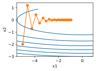
epoch 20, x1: -0.943467, x2: -0.000073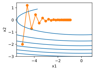
The gradient in the \(x_2\) direction is much larger and changes much faster than in \(x_1\), so one learning rate must accommodate both coordinates. A small rate prevents divergence in \(x_2\) but makes slow progress along \(x_1\). Raise it, and progress along \(x_1\) improves while \(x_2\) starts to oscillate out of control. Even the slight increase from \(0.4\) to \(0.6\) tips the balance:
eta = 0.6
d2l.show_trace_2d(f_2d, d2l.train_2d(gd_2d, f_grad=f_2d_grad))epoch 20, x1: -0.387814, x2: -1673.365109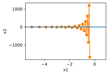
epoch 20, x1: -0.387814, x2: -1673.365109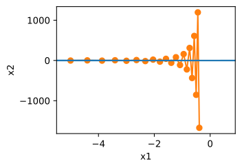
The trajectory history distinguishes these two directions. Along \(x_1\) successive gradients agree — small, but all pointing the same way. Along \(x_2\) they alternate in sign, each step undoing the last. An average over past gradients would amplify the first and cancel the second.
9.5.2 The Momentum Method
9.5.2.1 Leaky Averages
Minibatches (Section 9.4) average gradients across examples. The idea here is to also average across time, with an average that leaks: discount each past gradient by a factor of \(\beta\) per step. Concretely, replace the gradient in the update by a velocity \(\mathbf{v}_t\),
\[ \begin{aligned} \mathbf{v}_t &\leftarrow \beta \mathbf{v}_{t-1} + \mathbf{g}_{t}, \\ \mathbf{x}_t &\leftarrow \mathbf{x}_{t-1} - \eta\, \mathbf{v}_t, \end{aligned} \tag{9.5.2}\]
where \(\beta \in [0, 1)\), \(\mathbf{g}_t\) is the gradient — full-batch, single-example, or minibatch — evaluated at \(\mathbf{x}_{t-1}\), and \(\mathbf{v}_0 = \mathbf{0}\). For \(\beta = 0\) we recover plain gradient descent. Unrolling the recursion shows what the velocity holds:
\[\mathbf{v}_t = \sum_{\tau = 0}^{t-1} \beta^{\tau} \mathbf{g}_{t-\tau},\]
an exponentially weighted sum of all past gradients. The name comes from the physical picture: a heavy ball rolling down the objective integrates past forces rather than reacting to the instantaneous slope, and \(1 - \beta\) plays the role of friction. This is heavy-ball momentum, due to Polyak (1964); Sutskever et al. (2013) document how much it matters for training deep networks, and the expository article by Goh (2017) develops everything in this section with interactive animations.
9.5.2.2 Back to the Valley
On the valley, the leaky average does exactly what the trajectory history suggested: the persistent \(x_1\) components accumulate while the alternating \(x_2\) components cancel. At learning rate \(0.6\), for which plain gradient descent diverged, momentum \(\beta = 0.5\) converges well:
def momentum_2d(x1, x2, v1, v2, f_grad):
    g1, g2 = f_grad(x1, x2)
    v1, v2 = beta * v1 + g1, beta * v2 + g2
    return x1 - eta * v1, x2 - eta * v2, v1, v2

eta, beta = 0.6, 0.5
d2l.show_trace_2d(f_2d, d2l.train_2d(momentum_2d, f_grad=f_2d_grad))epoch 20, x1: 0.007188, x2: 0.002553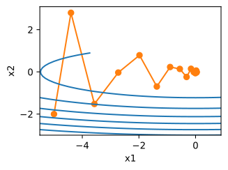
epoch 20, x1: 0.007188, x2: 0.002553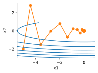
Reducing the momentum to \(\beta = 0.25\) weakens the effect, and the trajectory converges slowly. Plain gradient descent diverged at this learning rate:
eta, beta = 0.6, 0.25
d2l.show_trace_2d(f_2d, d2l.train_2d(momentum_2d, f_grad=f_2d_grad))epoch 20, x1: -0.126340, x2: -0.186632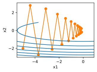
epoch 20, x1: -0.126340, x2: -0.186632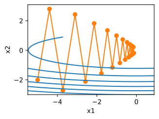
Nothing in Equation 9.5.2 requires the gradient to be exact. With minibatch gradients the same leaky average additionally smooths the sampling noise across steps. The velocity is therefore less noisy than a single minibatch gradient, at no extra gradient evaluations. Whether the iterates become less noisy as well depends on how \(\eta\) is adjusted along with \(\beta\), which Exercise 7 examines.
9.5.2.3 The Timescale of \(\beta\)
How much history does the velocity hold? The weights \(1, \beta, \beta^2, \ldots\) sum to \(\frac{1}{1-\beta}\) in the limit, so a useful reading is: momentum \(\beta\) averages over roughly the last \(\frac{1}{1-\beta}\) gradients. \(\beta = 0.9\) — the momentum=0.9 you have been passing to optimizers since Section 7.6 — looks back about \(10\) steps; \(\beta = 0.99\) about \(100\). The plot shows how sharply the weights decay for various \(\beta\):
d2l.set_figsize()
x = d2l.numpy(d2l.arange(40))
for beta in [0.95, 0.9, 0.6, 0]:
    d2l.plt.plot(x, beta ** x, label=f'beta = {beta:.2f}')
d2l.plt.xlabel('time')
d2l.plt.legend();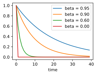
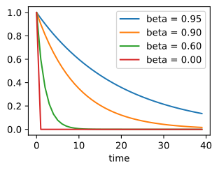
The same sum says something about step length. When successive gradients roughly agree, the velocity builds up to \(\frac{1}{1-\beta}\) times a typical gradient, so momentum takes steps of effective size \(\frac{\eta}{1-\beta}\) in persistent directions. This matters when tuning: raising \(\beta\) without lowering \(\eta\) makes the updates larger, not just smoother, and the two hyperparameters must move together — we will see this in the experiments below.
9.5.2.4 Acceleration and Damping
Momentum does more than stabilize; on ill-conditioned problems it is provably faster. For a quadratic whose Hessian eigenvalues lie between \(\mu\) and \(L\), the condition number \(\kappa = L/\mu\) governs the worst-case rate: gradient descent needs on the order of \(\kappa \log \frac{1}{\epsilon}\) iterations to reach precision \(\epsilon\), while heavy-ball momentum with optimally chosen \(\eta\) and \(\beta\) needs only on the order of \(\sqrt{\kappa} \log \frac{1}{\epsilon}\), achieved at
\[\beta^\star = \left(\frac{\sqrt{\kappa} - 1}{\sqrt{\kappa} + 1}\right)^{\!2}. \tag{9.5.3}\]
For \(\kappa = 100\) that is a \(10\times\) saving with \(\beta^\star \approx 0.67\); for \(\kappa = 10^4\), a \(100\times\) saving with \(\beta^\star \approx 0.96\). Note the trend: as \(\kappa\) grows, \(\beta^\star\) approaches \(1\). In the timescale interpretation, the optimum averages roughly \(\sqrt{\kappa}\) steps.
A damped oscillator provides a useful model for tuning \(\beta\). In each eigendirection of the Hessian, Equation 9.5.2 is a second-order recurrence — a mass on a spring with friction \(1 - \beta\). Too little momentum and the system is over-damped: it creeps down the valley like gradient descent. Too much and it is under-damped: the iterate overshoots and rings around the minimum. The fastest setting, \(\beta^\star\), sits at critical damping between the two. Our valley has \(\kappa = 20\), giving \(\beta^\star \approx 0.4\) — which is close to the earlier successful setting: \(\eta = 0.6\) with \(\beta = 0.5\). Push \(\beta\) too far and momentum turns against us. Here is \(\beta = 0.8\), well past the fastest-converging \(\beta^\star\), at a learning rate where plain gradient descent would be perfectly stable:
eta, beta = 0.3, 0.8
d2l.show_trace_2d(f_2d, d2l.train_2d(momentum_2d, f_grad=f_2d_grad))epoch 20, x1: 0.195696, x2: -0.249649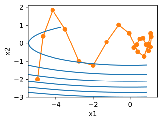
epoch 20, x1: 0.195696, x2: -0.249649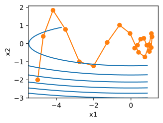
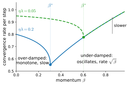
The trajectory advances along the valley but oscillates around the minimum before settling. This underdamped behavior differs from the earlier learning-rate divergence. Figure 9.5.1 summarizes the tradeoff on a single quadratic mode: the per-step convergence rate falls as \(\beta\) grows, is best at a critical value \(\beta^{*}\), and degrades gently past it. Section 26.1.4 develops the eigenmode analysis behind this picture, the \(\sqrt{\kappa}\) theorem and its matching lower bound, and the proofs. The scope of the result is important: the heavy-ball \(\sqrt{\kappa}\) rate is a statement about quadratics, and its practical standing on general objectives rests on the local quadratic approximation together with empirical evidence (Sutskever et al. 2013).
9.5.3 Implementation
9.5.3.1 From Scratch
Compared with plain minibatch SGD, momentum needs to maintain one auxiliary buffer per parameter — the velocity, with the same shape as the parameter. In the harness of Section 9.4 this is exactly what the states argument is for.
def init_momentum_states(feature_dim):
    v_w = d2l.zeros((feature_dim, 1))
    v_b = d2l.zeros(1)
    return (v_w, v_b)
def init_momentum_states(feature_dim):
v_w = d2l.zeros((feature_dim, 1))
v_b = d2l.zeros(1)
return [v_w, v_b]def sgd_momentum(params, states, hyperparams):
for p, v in zip(params, states):
with torch.no_grad():
v[:] = hyperparams['momentum'] * v + p.grad
p[:] -= hyperparams['lr'] * v
p.grad.zero_()def sgd_momentum(params, grads, states, hyperparams):
for i in range(len(params)):
states[i] = hyperparams['momentum'] * states[i] + grads[i]
params[i] = params[i] - hyperparams['lr'] * states[i]
return params[0], params[1]On the airfoil regression problem, a moderate \(\beta = 0.5\) with learning rate \(0.02\) trains without drama:
def train_momentum(lr, momentum, num_epochs=2):
    d2l.train_ch11(sgd_momentum, init_momentum_states(feature_dim),
                   {'lr': lr, 'momentum': momentum}, data_iter,
                   feature_dim, num_epochs)

data_iter, feature_dim = d2l.get_data_ch11(batch_size=10)
train_momentum(0.02, 0.5)loss: 0.246, 0.131 sec/epoch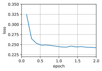
loss: 0.242, 1.116 sec/epoch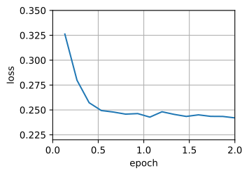
Raising the momentum to \(\beta = 0.9\) extends the average to roughly \(\frac{1}{1-0.9} = 10\) past gradients — and, by the effective-step reading above, quintuples the effective step \(\frac{\eta}{1-\beta}\) if we leave \(\eta\) alone. We halve the learning rate to \(0.01\) to rein it in:
train_momentum(0.01, 0.9)loss: 0.254, 0.088 sec/epoch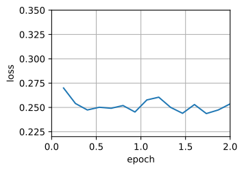
loss: 0.251, 0.332 sec/epoch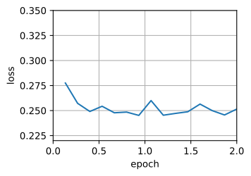
Halving it again to \(0.005\) brings the effective step to \(0.05\) — the range of the first experiment — and the loss curve settles accordingly:
train_momentum(0.005, 0.9)loss: 0.245, 0.080 sec/epoch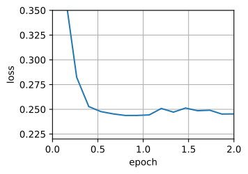
loss: 0.245, 0.324 sec/epoch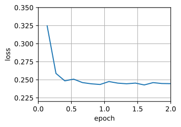
9.5.3.2 Concise Implementation
Momentum is built into every framework’s SGD optimizer as a single argument. Matching the hyperparameters reproduces the trajectory.
trainer = torch.optim.SGD
d2l.train_concise_ch11(trainer, {'lr': 0.005, 'momentum': 0.9}, data_iter)
loss: 0.246, 0.082 sec/epoch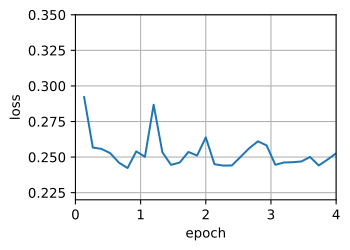
trainer = optax.sgd
d2l.train_concise_ch11(trainer, {'learning_rate': 0.005, 'momentum': 0.9},
                       data_iter)
loss: 0.249, 0.352 sec/epoch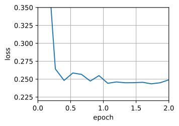
9.5.4 Nesterov Momentum
Heavy ball has one characteristic failure, and we have already seen it: with \(\beta\) past the critical value, the accumulated velocity overshoots and the iterate rings around the minimum. Nesterov (1983) proposed a fix of by evaluating the gradient at a look-ahead point. Evaluate the gradient not at the current point but at the point the velocity is about to carry you to:
\[ \begin{aligned} \mathbf{v}_t &\leftarrow \beta \mathbf{v}_{t-1} + \nabla f(\mathbf{x}_{t-1} - \eta \beta\, \mathbf{v}_{t-1}), \\ \mathbf{x}_t &\leftarrow \mathbf{x}_{t-1} - \eta\, \mathbf{v}_t. \end{aligned} \tag{9.5.4}\]
If the momentum step is about to overshoot, the gradient at the look-ahead point already points back, correcting the velocity before the mistake rather than one step after. In code it is a two-line change to the momentum update — the gradient is taken at the shifted point:
def nesterov_2d(x1, x2, v1, v2, f_grad):
    g1, g2 = f_grad(x1 - eta * beta * v1,  # Gradient at the look-ahead
                    x2 - eta * beta * v2)  # point, not at (x1, x2)
    v1, v2 = beta * v1 + g1, beta * v2 + g2
    return x1 - eta * v1, x2 - eta * v2, v1, v2

eta, beta = 0.3, 0.8
d2l.show_trace_2d(f_2d, d2l.train_2d(nesterov_2d, f_grad=f_2d_grad))epoch 20, x1: 0.217791, x2: -0.000070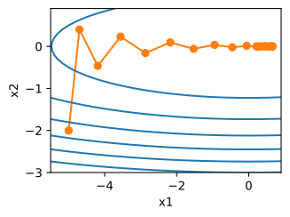
epoch 20, x1: 0.217791, x2: -0.000070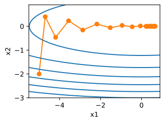
At the same learning rate and \(\beta = 0.8\) used for the oscillatory heavy-ball run, Nesterov momentum removes the visible oscillation: the look-ahead acts as built-in damping. Nesterov’s method also has guarantees beyond this quadratic example that heavy-ball momentum lacks. On smooth convex functions it converges as \(\mathcal{O}(1/k^2)\) against gradient descent’s \(\mathcal{O}(1/k)\), which is optimal for any method built from gradients; on strongly convex functions it achieves the \(\sqrt{\kappa}\) rate with a proof that is not confined to quadratics (Nesterov 2018). Statements, proofs, and the matching lower bound are in Section 26.1.4.
In frameworks, Nesterov momentum is one flag. Both PyTorch and Optax implement a rewrite of Equation 9.5.4 that evaluates the gradient at the parameters it stores, so no extra gradient evaluation is needed. Exercise 4 works out how those parameters relate to the iterates of Equation 9.5.4:
d2l.train_concise_ch11(
    torch.optim.SGD,
    {'lr': 0.005, 'momentum': 0.9, 'nesterov': True}, data_iter)
loss: 0.244, 0.080 sec/epoch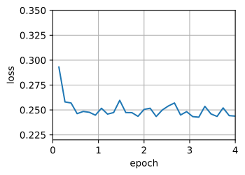
d2l.train_concise_ch11(
    optax.sgd,
    {'learning_rate': 0.005, 'momentum': 0.9, 'nesterov': True}, data_iter)
loss: 0.243, 0.343 sec/epoch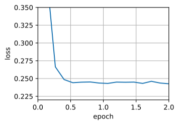
On this small, noisy problem the curve is nearly indistinguishable from plain momentum, as is typical at small batch: the look-ahead correction is dwarfed by sampling noise. The look-ahead correction matters most when curvature dominates noise, as in full-batch or large-batch training with \(\beta\) close to \(1\). Because it requires no additional gradient evaluation, implementations often enable it by default.
9.5.5 Summary
Momentum replaces the gradient with a leaky average over past gradients. It adds one buffer and one hyperparameter, \(\beta\). On ill-conditioned problems it cures the zigzag: persistent gradient components accumulate up to \(\frac{1}{1-\beta}\)-fold while oscillating ones cancel, and with optimal tuning the iteration count improves from order \(\kappa\) to order \(\sqrt{\kappa}\). The parameter \(\beta\) reads as a timescale — an average over roughly \(\frac{1}{1-\beta}\) recent gradients — and as a damping knob, with too large a value producing ringing rather than progress. Nesterov’s look-ahead variant damps that ringing and carries convergence guarantees beyond quadratics, at no extra cost per step. With stochastic gradients the same leaky average also smooths the sampling noise in the velocity, which is why some form of momentum appears in most optimizers considered in the rest of this chapter.
9.5.6 Exercises
- [code] Momentum and learning rate together. On the valley
f_2dwithmomentum_2d, run a grid of \(\beta \in \{0, 0.25, 0.5, 0.8\}\) and \(\eta \in \{0.1, 0.3, 0.6, 1.0\}\) for up to 1000 steps each.- Record for every cell the number of steps until \(\|\mathbf{x}_t\| \leq 10^{-3}\), or the fact that the iterates diverged, and display the grid as a table or heatmap.
- Compare the fastest \(\beta\) at each stable \(\eta\) with the \(\beta^\star\) of Section 9.5.2.4 for \(\kappa = 20\), and explain each learning rate at which they differ.
- Stability of momentum. ● The effective-step reading of Section 9.5.2.3 suggests that raising \(\beta\) forces \(\eta\) down. Does the largest stable \(\eta\) in the grid of the previous problem behave that way? Derive the stability condition of Equation 9.5.2 for a single eigendirection with curvature \(\lambda\) and reconcile the two.
- [code] Many eigenvalues. ● Consider \(f(\mathbf{x}) = \frac{1}{2} \sum_{i=1}^{10} \lambda_i x_i^2\) with \(\lambda_i = 2^{-i}\), started from \(x_i = 1\). Let \(L\) and \(\mu\) be the largest and the smallest \(\lambda_i\), and let \(\kappa = L/\mu\).
- Run gradient descent at \(\eta = 2/(L + \mu)\), the learning rate that minimizes its worst-case contraction factor \(\max_i |1 - \eta\lambda_i|\). Run heavy-ball momentum at \(\eta = 4/(\sqrt{L} + \sqrt{\mu})^2\) with the \(\beta^\star\) of Section 9.5.2.4. Plot \(|x_{i,t}|\) for every coordinate on a logarithmic scale.
- Which coordinates limit the convergence of each method? Compare the ratio of the iteration counts until \(\|\mathbf{x}_t\| \leq 10^{-6}\) with \(\sqrt{\kappa}\).
- Two forms of Nesterov momentum. Library implementations of Nesterov momentum store a parameter vector \(\mathbf{y}_t\) and evaluate the gradient there, \(\mathbf{g}_t = \nabla f(\mathbf{y}_{t-1})\). Starting from \(\mathbf{y}_0 = \mathbf{x}_0\) and \(\mathbf{v}_0 = \mathbf{0}\), they update \[\mathbf{v}_t = \beta \mathbf{v}_{t-1} + \mathbf{g}_t, \qquad
\mathbf{y}_t = \mathbf{y}_{t-1} - \eta\,(\mathbf{g}_t + \beta \mathbf{v}_t),\] so that no extra gradient evaluation is needed.
- Express \(\mathbf{y}_t\) through the \(\mathbf{x}_t\) and \(\mathbf{v}_t\) of Equation 9.5.4 so that both recurrences produce the same velocities, and prove the relation by induction over \(t\).
- A checkpoint saves the library’s parameters \(\mathbf{y}_t\). Which point of Equation 9.5.4 does it store, and what else must be saved to recover \(\mathbf{x}_t\)?
- [code] Critical damping. For \(f(x) = \frac{\lambda}{2} x^2\) at a fixed learning rate with \(\eta\lambda = 0.1\), sweep \(\beta\) over \([0, 1)\) in steps of \(0.02\) and measure the number of iterations after which \(|x_t|\) stays at or below \(10^{-6} |x_0|\).
- Locate the minimizing \(\beta\) and compare it with the critical value \(\beta^\star = (1 - \sqrt{\eta\lambda})^2\) at which the recurrence Equation 9.5.2 for this mode is critically damped.
- Describe the iterates on either side of \(\beta^\star\) and match them with the over-damped and under-damped regimes of Figure 9.5.1.
- Velocity noise. Let \(\mathbf{g}_t = \mathbf{g} + \boldsymbol{\xi}_t\), where the noise \(\boldsymbol{\xi}_t\) is independent across steps, has zero mean, and has variance \(\sigma^2\) per coordinate. Show that the stationary mean of \(\mathbf{v}_t\) in Equation 9.5.2 is \(\mathbf{g}/(1-\beta)\) and its stationary variance is \(\sigma^2/(1-\beta^2)\). Conclude that the noise-to-signal ratio of the velocity is \(\sqrt{(1-\beta)/(1+\beta)}\) times that of a single gradient.
- [code] Momentum under minibatch noise. ● Keep the noise model of the previous problem, but let the gradient depend on the iterate: on \(f(x) = \frac{\lambda}{2} x^2\), take \(g_t = \lambda x_{t-1} + \xi_t\).
- Compare plain SGD at learning rate \(\alpha\) with momentum \(\beta = 0.9\) at \(\eta = \alpha (1-\beta)\), which keeps the effective step \(\frac{\eta}{1-\beta}\) equal to \(\alpha\). Compute the ratio of the two stationary variances of \(x_t\) for \(\alpha\lambda \in \{0.05, 0.2\}\), by simulation or by solving for the stationary covariance of \((x_t, v_t)\). Does the reduction of the velocity’s noise-to-signal ratio from the previous problem carry over to the iterate? Explain the result.
- On the airfoil harness, rebuild
data_iterandfeature_dimwithd2l.get_data_ch11(batch_size=b)for \(b \in \{1, 10, 100\}\). Rund2l.train_ch11withsgd_momentumandnum_epochs=10at \(\beta \in \{0, 0.9\}\), choosing \(\eta\) so that \(\eta/(1-\beta) = 0.05\). Report the final loss of each run and the spread of the recorded losses over its last epoch, and compare the effect of momentum with the prediction of the first item.