%matplotlib inline
from d2l import torch as d2l
import numpy as np8.6 Backpropagation Through Time
Gradient clipping keeps the occasional enormous gradient from destabilizing RNN training. You met it in Section 8.5, where we hinted that these blow-ups come from backpropagating across long sequences. Before turning to the modern architectures of Chapter 12, let us look closely at how backpropagation actually works in a sequence model, so that vanishing and exploding gradients become precise phenomena rather than slogans.
Forward propagation in an RNN iterates over time while reusing the same parameters. Applying backpropagation to this recurrent computation is called backpropagation through time (Werbos 1990): we unroll the computational graph one step at a time into an ordinary feedforward network, then apply the chain rule, remembering that the same parameters reappear at every step, so their gradients are summed over all those occurrences (the weight tying is exactly as in a convolutional network). Long sequences create both computational and numerical problems. A text sequence can run to thousands of tokens; the input at step 1 then passes through a thousand matrix products before it reaches the output, and another thousand to compute the gradient. This is costly in memory and, as we will see, numerically treacherous.
%matplotlib inline
from d2l import tensorflow as d2l
import numpy as np%matplotlib inline
from d2l import jax as d2l
import numpy as np%matplotlib inline
from d2l import mxnet as d2l
import numpy as np8.6.1 The Unrolled Graph and the Full Gradient
We first use scalar notation to expose the dependency structure. Write \(h_t,x_t,o_t\in\mathbb{R}\) for the state, input, and output, and let \(w_\textrm{h},w_\textrm{o}\in\mathbb{R}\) denote shared parameters. The vector case replaces each derivative below with a Jacobian; its dimensions are given when we specialize to a linear RNN. Then
\[ \begin{aligned}h_t &= f(x_t, h_{t-1}, w_\textrm{h}),\\ o_t &= g(h_t, w_\textrm{o}),\end{aligned} \tag{8.6.1}\]
and the loss over all \(T\) steps is \(L = \frac{1}{T}\sum_{t=1}^T l(y_t, o_t)\).
Forward propagation just walks the chain of \((x_t, h_t, o_t)\) triples. The gradient with respect to the output weights \(w_\textrm{o}\) is easy. The trouble is \(w_\textrm{h}\), because it feeds every hidden state. By the chain rule,
\[ \frac{\partial L}{\partial w_\textrm{h}} = \frac{1}{T}\sum_{t=1}^T \frac{\partial l(y_t, o_t)}{\partial o_t}\, \frac{\partial g(h_t, w_\textrm{o})}{\partial h_t}\, \frac{\partial h_t}{\partial w_\textrm{h}}. \tag{8.6.2}\]
The first two factors are local. The third, \(\partial h_t/\partial w_\textrm{h}\), is the hard one, because \(h_t\) depends on \(w_\textrm{h}\) both directly and through \(h_{t-1}\), which depends on \(w_\textrm{h}\) in turn:
\[ \frac{\partial h_t}{\partial w_\textrm{h}} = \frac{\partial f(x_t,h_{t-1},w_\textrm{h})}{\partial w_\textrm{h}} + \frac{\partial f(x_t,h_{t-1},w_\textrm{h})}{\partial h_{t-1}}\, \frac{\partial h_{t-1}}{\partial w_\textrm{h}}. \tag{8.6.3}\]
To unwind this recursion, use a small lemma: if \(a_t = b_t + c_t a_{t-1}\) with \(a_0 = 0\), then for \(t \geq 1\)
\[ a_t = b_t + \sum_{i=1}^{t-1}\Big(\prod_{j=i+1}^{t} c_j\Big) b_i. \tag{8.6.4}\]
Substituting \(a_t = \partial h_t/\partial w_\textrm{h}\), \(b_t = \partial f/\partial w_\textrm{h}\), and \(c_t = \partial f/\partial h_{t-1}\) turns the recursion Equation 8.6.3 into a closed form:
\[ \frac{\partial h_t}{\partial w_\textrm{h}} = \frac{\partial f(x_t,h_{t-1},w_\textrm{h})}{\partial w_\textrm{h}} + \sum_{i=1}^{t-1}\Big(\prod_{j=i+1}^{t} \frac{\partial f(x_j,h_{j-1},w_\textrm{h})}{\partial h_{j-1}}\Big) \frac{\partial f(x_i,h_{i-1},w_\textrm{h})}{\partial w_\textrm{h}}. \tag{8.6.5}\]
The gradient of a recurrence, in three equations. Equation Equation 8.6.1 is the forward recurrence; Equation 8.6.3 is its gradient, one step at a time; and Equation 8.6.5 is that gradient unrolled. The last one is the object of study for the rest of this section. Its second term is a sum over all earlier steps \(i\), and each summand carries a product of Jacobians \(\prod_{j=i+1}^{t} \partial f/\partial h_{j-1}\) that reaches back from step \(t\) to step \(i\). Computing this sum in full is exact, but the work grows with \(t\), and, as the next section shows, those long products are exactly where the numbers go wrong.
8.6.2 Vanishing and Exploding Gradients
The numerical difficulty comes from the product of state Jacobians \(\prod_{j=i+1}^{t} \partial f/\partial h_{j-1}\) in Equation 8.6.5. To see what it does, make the recurrence concrete: drop the biases and the nonlinearity so that the hidden layer is a plain linear map,
\[ \mathbf{h}_t = \mathbf{W}_\textrm{hx}\mathbf{x}_t + \mathbf{W}_\textrm{hh}\mathbf{h}_{t-1}, \qquad \mathbf{o}_t = \mathbf{W}_\textrm{qh}\mathbf{h}_t, \]
with \(\mathbf{W}_\textrm{hx}\in\mathbb{R}^{h\times d}\), \(\mathbf{W}_\textrm{hh}\in\mathbb{R}^{h\times h}\), and \(\mathbf{W}_\textrm{qh}\in\mathbb{R}^{q\times h}\). Figure 8.6.1 draws the resulting dependencies: each \(\mathbf{h}_t\) feeds both the output \(\mathbf{o}_t\) and the next state \(\mathbf{h}_{t+1}\).
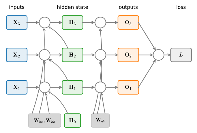
Now every Jacobian \(\partial\mathbf{h}_{j}/\partial\mathbf{h}_{j-1}\) is the same matrix \(\mathbf{W}_\textrm{hh}\). Propagating the loss gradient backwards, the hidden state at step \(t\) collects a contribution from its own output and one from the next step,
\[ \frac{\partial L}{\partial \mathbf{h}_t} = \mathbf{W}_\textrm{hh}^\top \frac{\partial L}{\partial \mathbf{h}_{t+1}} + \mathbf{W}_\textrm{qh}^\top \frac{\partial L}{\partial \mathbf{o}_t}, \tag{8.6.6}\]
which unrolls (this is Equation 8.6.4 again, now with matrices) to
\[ \frac{\partial L}{\partial \mathbf{h}_t} = \sum_{i=t}^T \big(\mathbf{W}_\textrm{hh}^\top\big)^{T-i}\, \mathbf{W}_\textrm{qh}^\top\, \frac{\partial L}{\partial \mathbf{o}_{T+t-i}}. \tag{8.6.7}\]
There it is: the gradient that reaches back \(k = T-i\) steps is multiplied by the \(k\)-th power \((\mathbf{W}_\textrm{hh}^\top)^{k}\). A matrix power is governed by its eigenvalues. Write \(\rho(\mathbf{W}_\textrm{hh})\) for the spectral radius, the largest eigenvalue magnitude; the contribution from \(k\) steps back then scales roughly as \(\rho^{k}\): eigen-directions with \(|\lambda|<1\) shrink geometrically and vanish, those with \(|\lambda|>1\) grow geometrically and explode, and only \(\rho\) exactly at \(1\) sits on the knife-edge. The parameter gradients \(\partial L/\partial\mathbf{W}_\textrm{hx}\) and \(\partial L/\partial\mathbf{W}_\textrm{hh}\) are just sums of these hidden-state gradients weighted by an input or a previous state, so they inherit the same fate.
We can watch it happen. Take a random symmetric recurrence \(\mathbf{J}=\mathbf{W}_\textrm{hh}\) (symmetric so that its singular values equal its eigenvalue magnitudes and \(\|\mathbf{J}^k\|=\rho^k\) exactly), rescale it to a chosen spectral radius \(\rho\), and measure the operator norm \(\|\mathbf{J}^k\|\) of its \(k\)-step Jacobian product as the lag \(k\) grows.
np.random.seed(1)
h = 100
M = np.random.randn(h, h)
W = M + M.T                                # a random *symmetric* recurrence

def spectral_radius(A):
    return np.abs(np.linalg.eigvals(A)).max()

lags, norms = np.arange(41), []
for rho in (0.9, 1.0, 1.1):
    J = W * (rho / spectral_radius(W))     # rescale so that rho(J) = rho
    power, seq = np.eye(h), []
    for k in lags:
        seq.append(np.linalg.norm(power, 2))   # operator norm of J^k
        power = power @ J
    norms.append(seq)
    print(f'rho={rho}: ||J^40|| = {seq[-1]:.3g}')

d2l.plot(lags, norms, xlabel='time lag $k$', ylabel=r'$\|\mathbf{J}^k\|$',
         legend=[r'$\rho=0.9$ (vanish)', r'$\rho=1.0$', r'$\rho=1.1$ (explode)'],
yscale='log', figsize=(4.5, 3))rho=0.9: ||J^40|| = 0.0148
rho=1.0: ||J^40|| = 1
rho=1.1: ||J^40|| = 45.3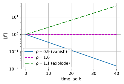
rho=0.9: ||J^40|| = 0.0148
rho=1.0: ||J^40|| = 1
rho=1.1: ||J^40|| = 45.3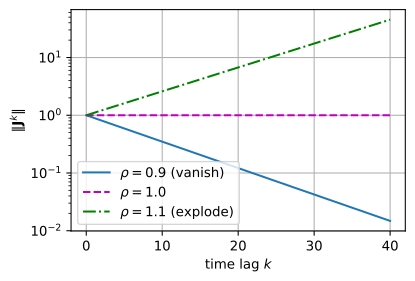
rho=0.9: ||J^40|| = 0.0148
rho=1.0: ||J^40|| = 1
rho=1.1: ||J^40|| = 45.3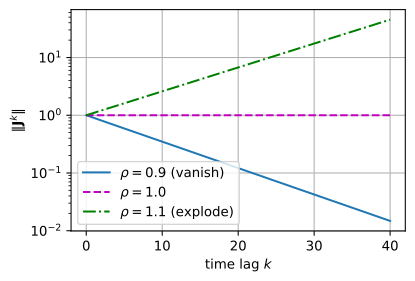
rho=0.9: ||J^40|| = 0.0148
rho=1.0: ||J^40|| = 1
rho=1.1: ||J^40|| = 45.3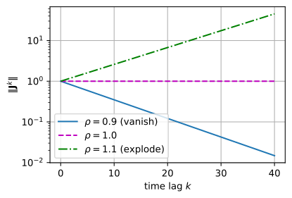
The three regimes are geometric and could not be cleaner: at \(\rho=0.9\) the norm decays toward zero, at \(\rho=1.1\) it grows without bound, and only \(\rho=1.0\) holds steady. Over forty steps a signal is amplified more than fortyfold or shrunk below two percent; either way, the gradient that finally arrives says almost nothing reliable about a dependency that far back. A general, non-symmetric \(\mathbf{W}_\textrm{hh}\) adds transient wobbles on top, but the same \(\rho^k\) trend wins in the end.
8.6.2.1 From Arithmetic to Architecture
The two failure modes call for two very different remedies. Explosion is the easy one: a gradient that is merely too large still points in a useful direction, so we simply rescale it. That is gradient clipping (Section 8.5), which caps the norm of the gradient before each update and reliably tames the rare blow-ups. Vanishing is the hard one, and no rescaling can fix it: once the signal from a distant step has decayed into numerical noise the information is gone, and scaling up noise only gives you bigger noise. The cure has to change the dynamics of the recurrence so that the Jacobian product stops shrinking in the first place, and this is an architectural question, not an arithmetic one. Two ideas answer it, and the rest of this part is built on them. The first is gating (Section 12.1): the cell carries a near-identity path along which the relevant Jacobian stays close to the identity, so gradients neither vanish nor explode as they travel along it. The second is to give up the nonlinearity in the state update altogether and use a linear recurrence whose state-to-state map is reparameterized so that its eigenvalues are pinned just inside the unit circle by construction, making \(\rho \le 1\) a guarantee rather than a hope; this is the route the linear recurrences and state space models of Chapter 12 take. Both replace the vanilla RNN’s fragile, learned-by-accident dynamics with a memory path that is stable by design, and both trace directly back to the product of Jacobians we have just analyzed.
8.6.3 Truncated Backpropagation Through Time
Summing Equation 8.6.5 in full is exact, but its cost grows with the sequence length and, as we just saw, it drags along the whole vanishing/exploding pathology. The standard practical answer is to truncate: stop the sum after \(\tau\) steps, equivalently detaching the hidden state every \(\tau\) steps so that no gradient flows across the boundary. Figure 8.6.2 contrasts the two.
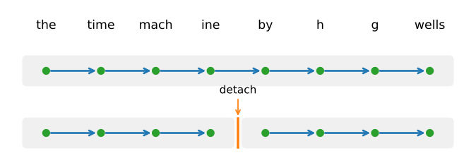
Truncation introduces a real bias. The model only ever sees dependencies inside a window of \(\tau\) steps and literally cannot learn a coupling longer than that, so its gradient is a truncated approximation of the true one (Jaeger 2002). Often this is harmless or even helpful: shorter windows bias the estimate toward simpler, more stable, better-generalizing models, a mild regularizer. But it is a genuine ceiling on the memory the model can be trained to use, and it is one of the reasons we reach for the architectures above. In code, truncation is not a change to the loss but the one-line detach-state idiom: detach the hidden state from the graph at each chunk boundary before continuing the forward pass. The language model of Section 8.5 needs no detach, because each of its windows starts from a zero state; the idiom matters once the state is carried across consecutive chunks. One can instead truncate at random lengths chosen so the estimator stays unbiased in expectation (Tallec and Ollivier 2017), but the extra variance rarely pays for itself and regular truncation remains the default.
The store-versus-recompute trade-off behind truncation reaches far beyond RNNs. Backpropagation of any kind must keep intermediate activations around to reuse on the backward pass, and for very deep or very long models that storage becomes the binding constraint. Activation checkpointing applies the same idea to depth rather than time: keep only a sparse set of activations on the forward pass and recompute the rest on demand during backpropagation, spending extra compute to shrink the memory footprint. It is the technique that lets today’s largest models fit in memory, and we will meet it again in the chapters on large-scale model training.
8.6.4 Summary
Backpropagation through time is nothing more than backpropagation applied to a sequence model with a hidden state: unroll the recurrence, apply the chain rule, and sum each shared parameter’s gradient over every step at which it acts. The gradient that reaches back \(k\) steps carries a \(k\)-fold product of state-to-state Jacobians, so in the linear case it scales like the \(k\)-th power of \(\mathbf{W}_\textrm{hh}\). Eigenvalues below one make that product vanish and eigenvalues above one make it explode, which is precisely vanishing and exploding gradients. Clipping controls explosion; only a change of architecture, gating or a stably parameterized linear recurrence, controls vanishing. In practice we truncate the backward pass to a fixed horizon, trading a little bias for a lot of stability and memory, the same store-versus-recompute bargain that reappears as activation checkpointing at scale.
8.6.5 Exercises
Backward pass by hand. One step of
RNNScratch(Section 8.5) computes \[\mathbf{H}_t = \tanh(\mathbf{X}_t \mathbf{W}_{\textrm{xh}} + \mathbf{H}_{t-1} \mathbf{W}_{\textrm{hh}} + \mathbf{b}_\textrm{h}).\] Let \(\mathbf{G}_t = \partial L / \partial \mathbf{H}_t\) be the gradient arriving from later steps and from the output at step \(t\).
- Derive the contributions of this step to \(\partial L / \partial \mathbf{W}_{\textrm{xh}}\), \(\partial L / \partial \mathbf{W}_{\textrm{hh}}\), \(\partial L / \partial \mathbf{b}_\textrm{h}\), and \(\partial L / \partial \mathbf{H}_{t-1}\) as functions of \(\mathbf{G}_t\), \(\mathbf{X}_t\), \(\mathbf{H}_t\), \(\mathbf{H}_{t-1}\), and \(\mathbf{W}_{\textrm{hh}}\).
- Adding the output contribution at step \(t-1\) to the contribution to \(\partial L / \partial \mathbf{H}_{t-1}\) gives a recursion for \(\mathbf{G}_{t-1}\). Equation Equation 8.6.6 uses column vectors, so its \(\mathbf{W}_\textrm{hh}\) is the transpose of
W_hhinRNNScratch. Show that the recursion reduces to that equation when the \(\tanh\) is dropped, and name the factor that the \(\tanh\) adds at every step. Explain also how the parameter gradients accumulate over the \(T\) steps of a window.
Adapted from CMU 11-785, Homework 3 Part 1.
[code] Backward pass in code. ● Train
d2l.RNNLMScratchond2l.TimeMachineas in Section 8.5. Using the single-step gradients and the recursion of the previous problem, implement the backward pass of itsRNNScratchcell over a full window with tensor operations only, starting from the gradient of the loss with respect to the logits (Section 3.1.3.2). Run it on one training minibatch, and compare your gradients ofW_xh,W_hh, andb_hwith those computed by automatic differentiation.Adapted from CMU 11-785, Homework 3 Part 1.
Power iteration and alignment. Let \(\mathbf{M} \in \mathbb{R}^{n \times n}\) be symmetric with eigenvalues \(\lambda_i\) and eigenvectors \(\mathbf{v}_i\) for \(i = 1, \ldots, n\), ordered so that \(|\lambda_i| \geq |\lambda_{i+1}|\).
- Show that \(\mathbf{M}^k\) has eigenvalues \(\lambda_i^k\) with the same eigenvectors.
- Show that for a random vector \(\mathbf{x} \in \mathbb{R}^n\) with independent standard normal entries, \(\mathbf{M}^k \mathbf{x}\) becomes aligned with \(\mathbf{v}_1\) as \(k\) grows. State the condition on the eigenvalues that this requires and the sense in which the alignment holds.
- What does this imply for the gradient Equation 8.6.7 of an RNN, beyond the change in its norm?
[code] Nonlinear Jacobians. ● Rerun the experiment of Section 8.6.2 at the same three spectral radii with two changes.
- Replace the symmetric matrix by a general, non-symmetric \(\mathbf{W}_\textrm{hh}\) rescaled to each radius, and plot \(\|\mathbf{J}^k\|\) against \(k\). Report the largest value of \(\|\mathbf{J}^k\|\) at \(\rho = 0.9\) and the lag at which it occurs. Explain why the ratio \(\|\mathbf{J}^k\| / \rho^k\) can exceed one and why it stays bounded as \(k\) grows.
- Return to the symmetric \(\mathbf{W}_\textrm{hh}\) and run the \(\tanh\) RNN \[\mathbf{h}_t = \tanh(\mathbf{W}_\textrm{hh}\mathbf{h}_{t-1} + \mathbf{x}_t), \qquad \mathbf{h}_0 = \mathbf{0}, \tag{8.6.8}\] with inputs \(\mathbf{x}_t \sim \mathcal{N}(\mathbf{0}, s^2\mathbf{I})\). Plot the norm of the product of the Jacobians \(\partial \mathbf{h}_j / \partial \mathbf{h}_{j-1}\) along the trajectory for \(s = 0.1\) and \(s = 1\). How do the nonlinearity and the input scale change the growth of the norm, and why?
- Explain why a largest singular value of \(\mathbf{W}_\textrm{hh}\) below one is sufficient for the product to shrink, whereas a largest singular value above one is necessary but not sufficient for it to grow (Bengio et al. 1994; Pascanu et al. 2013). Relate the argument to your \(\tanh\) curves at \(\rho = 0.9\) and \(\rho = 1.1\).
Beyond clipping. Propose two methods for coping with exploding gradients in a vanilla RNN other than clipping, truncation, and the two architectural remedies of
Section 8.6.2.1. One method should act on the parameters and the other on the optimizer step. For each, state whether it changes the Jacobian product in Equation 8.6.7 or only limits what a large gradient does to the update, and whether it also helps against vanishing gradients. If it changes the product, name the property of the product that it controls.
[code] Effective memory horizon. ● Take the RNN language model trained in Section 8.5 and a fixed input sequence of several hundred tokens. Measure the norm of the gradient of the loss at the final step with respect to the hidden state \(k\) steps earlier, as a function of \(k\), and plot it.
- Read off the lag beyond which the norm drops below one percent of its value at \(k = 0\).
- Compare this horizon with the window length
num_stepsused in training. Which of the two, the truncation atnum_stepsor the decay of the gradient, limits the longest dependency the model could have learned? - Retrain with
num_stepsset to 128, measure the horizon again, and explain the change or its absence in terms of the product of state Jacobians in Equation 8.6.5.