from d2l import torch as d2l
import math
import torch
from torch import nn
from torch.nn import functional as F7.6 Modern Training Recipes for Convnets
Take the ResNet-50 of Section 7.4, change nothing about its architecture, and train it with the methods in use around 2022 instead of those of its 2015 debut. Its ImageNet top-1 accuracy rises from 76.1% to 80.4% (Wightman et al. 2021). That gain, from the training recipe alone, exceeds what most new architectures delivered over their predecessors. The “ResNet strikes back” study that produced it trained the unmodified network with three procedures of increasing cost: A3 (100 epochs) reaches 78.1%, A2 (300 epochs) reaches 79.8%, and A1 (600 epochs, the LAMB optimizer, a binary cross-entropy loss, and heavy augmentation) reaches 80.4%.
Consequently, ResNet-50 results obtained with training procedures from different periods are not directly comparable. Some gains initially attributed to architecture were later reproduced by changes in optimization and data augmentation. We examine the main changes between 2015 and 2022, implement each component, and compare two training procedures on the same ResNet-18.
import math
import tensorflow as tf
from d2l import tensorflow as d2l
from d2l import jax as d2l
from flax import nnx
import jax
from jax import numpy as jnp
import math
import optaxfrom d2l import mxnet as d2l
import math
import mxnet as mx
from mxnet import autograd, np, npx
npx.set_np()7.6.1 What Changed between 2015 and 2022
The original ResNet recipe was already careful: SGD with momentum, weight decay, a learning rate dropped by a factor of 10 twice during training, and random crops and horizontal flips as augmentation (He et al. 2016). Between then and roughly 2022, every one of those choices was revisited. The first systematic accounting, in 2019, collected the accumulated techniques (warmup, cosine decay, label smoothing, Mixup, zero-initializing the last batch-norm scale in each block) and showed that stacking them, plus a small tweak to the downsampling path, lifts ResNet-50 from 75.3% to 79.3% (He et al. 2019), an early sign that the recipe rivals the architecture. Table 7.6.1 summarizes the full shift.
:A 2015 ImageNet recipe and a representative high-accuracy recipe from the early 2020s. The later column is not a universal standard; strong recipes still vary by model and compute budget.
| Ingredient | 2015 recipe | 2022 recipe |
|---|---|---|
| Optimizer | SGD with momentum | AdamW or LAMB; tuned SGD remains competitive |
| Schedule | step decay (drop by 10x twice) | cosine decay with linear warmup |
| Augmentation | random crops, horizontal flips | RandAugment, Mixup, CutMix, random erasing |
| Regularization | weight decay | + label smoothing, stochastic depth |
| Duration | 90 epochs | 300 to 600 epochs |
| Evaluated weights | final checkpoint | exponential moving average of weights |
The optimizer row shows one common change, from SGD to AdamW (Loshchilov and Hutter 2019), rather than a universal replacement. Earlier Adam implementations folded weight decay into the gradient, where adaptive rescaling distorts it. AdamW decouples the weight update from the gradient and made adaptive methods competitive with tuned SGD on many vision recipes. At batch sizes in the tens of thousands, layerwise rescaling of the update can keep training stable, as in LARS (You et al. 2017) and its Adam-based sibling LAMB, used for recipe A1 above.
The schedule row replaces discrete drops with a smooth cosine decay (Loshchilov and Hutter 2016), preceded by a few epochs of linear warmup that protect the network from divergence while its randomly initialized layers produce large, poorly scaled gradients. We implement and plot it below.
The augmentation and regularization rows account for much of the accuracy improvement. RandAugment (Cubuk et al. 2020) applies randomly chosen image transformations at a single tuned strength; Mixup (Zhang et al. 2018) and CutMix (Yun et al. 2019) blend pairs of training images and their labels; label smoothing (Szegedy et al. 2016) softens the targets themselves; stochastic depth (Huang et al. 2016) randomly skips whole residual blocks during training. These methods alter the training targets, examples, or computation and generally require longer optimization; accordingly, the duration row grows from 90 epochs to several hundred. A heavily regularized short run underperforms an unregularized one; regularization and duration must move together.
The final row changes what gets evaluated. Instead of the last iterate of a noisy stochastic optimization, modern recipes evaluate an exponential moving average (EMA) of the weights, a cheap online cousin of the averaging schemes studied by Izmailov et al. (2018) . It typically adds a few tenths of a point for one extra copy of the parameters.
None of these ideas is deep in isolation. Their compounded effect, four points of ImageNet top-1 on a fixed network, is what earns them a section of their own.
7.6.2 Implementing the Ingredients
Each ingredient is a few lines of code. We implement label smoothing, the cosine schedule, Mixup, stochastic depth, and the weight EMA; RandAugment is a library call in practice (its contribution is the tuning of augmentation strength, not the code) and we omit it here.
7.6.2.1 Label Smoothing
Cross-entropy training with one-hot targets never converges in the logits: the loss keeps decreasing as the correct-class logit grows without bound, so the network is rewarded for unbounded overconfidence. Label smoothing replaces the one-hot target with a mixture that puts weight \(1-\epsilon\) on the label and spreads \(\epsilon\) uniformly over all \(K\) classes. Writing \(p_k\) for the predicted softmax probabilities, the loss on an example with label \(y\) becomes
\[ \ell_\epsilon = -(1-\epsilon) \log p_y - \frac{\epsilon}{K} \sum_{k=1}^K \log p_k. \tag{7.6.1}\]
The minimizer places probability \(1-\epsilon+\epsilon/K\) on the correct class and \(\epsilon/K\) on every other class, which requires only a finite logit gap. We can see the effect directly: on a prediction that is already extremely confident and correct, the unsmoothed loss is nearly zero, while the smoothed loss is bounded away from zero. The optimizer therefore stops pushing confident examples harder and spends its effort elsewhere.
logits, y = d2l.tensor([[10.0, 0.0, 0.0]]), d2l.tensor([0])
for epsilon in (0.0, 0.1):
    loss = F.cross_entropy(logits, y, label_smoothing=epsilon)
    print(f'epsilon={epsilon}: loss={float(loss):.4f}')
epsilon=0.0: loss=0.0001
epsilon=0.1: loss=0.6668logits, Y = tf.constant([[10.0, 0.0, 0.0]]), tf.one_hot([0], 3)
for epsilon in (0.0, 0.1):
loss = tf.keras.losses.CategoricalCrossentropy(
from_logits=True, label_smoothing=epsilon)(Y, logits)
print(f'epsilon={epsilon}: loss={float(loss):.4f}')epsilon=0.0: loss=0.0001
epsilon=0.1: loss=0.6668logits, Y = jnp.array([[10.0, 0.0, 0.0]]), jax.nn.one_hot(jnp.array([0]), 3)
for epsilon in (0.0, 0.1):
loss = optax.softmax_cross_entropy(
logits, optax.smooth_labels(Y, alpha=epsilon)).mean()
print(f'epsilon={epsilon}: loss={float(loss):.4f}')epsilon=0.0: loss=0.0001
epsilon=0.1: loss=0.6668def smoothed_ce(y_hat, y, epsilon):
logp = npx.log_softmax(y_hat)
return -(1 - epsilon) * npx.pick(logp, y) - epsilon * logp.mean(axis=1)
logits, y = np.array([[10.0, 0.0, 0.0]]), np.array([0])
for epsilon in (0.0, 0.1):
loss = float(smoothed_ce(logits, y, epsilon).mean())
print(f'epsilon={epsilon}: loss={loss:.4f}')epsilon=0.0: loss=0.0001
epsilon=0.1: loss=0.66687.6.2.2 Cosine Schedules with Warmup
A step schedule holds the learning rate constant for tens of epochs and then drops it by a factor of 10, an abrupt change whose timing is two extra hyperparameters. The modern default replaces it with two phases: a linear warmup from zero over the first few epochs, then a half-cosine decay from the base rate \(\eta_0\) to (nearly) zero,
\[ \eta_t = \frac{\eta_0}{2} \left(1 + \cos \frac{\pi (t - t_{\textrm{w}})}{T - t_{\textrm{w}}}\right) \quad \textrm{for } t \geq t_{\textrm{w}}, \tag{7.6.2}\]
where \(t_{\textrm{w}}\) is the warmup length and \(T\) the total budget. Warmup exists because a freshly initialized network produces large, badly scaled gradients; a few gentle epochs let the running statistics of batch normalization and of the optimizer settle before full-strength updates arrive. The cosine tail matters at the other end: the long stretch of small learning rates is when the noisy iterates settle into a low-loss region, and with Mixup-style augmentation most of the measurable accuracy gain arrives in exactly that tail. Both schedules are one-liners; we plot them for a 45-epoch budget.
def step_decay(epoch, max_epochs, base_lr):
    """Recipe A: multiply the rate by 0.1 at 60% and 85% of the budget."""
    return base_lr * 0.1 ** sum(epoch >= int(f * max_epochs)
                                for f in (0.6, 0.85))

def cosine_warmup(epoch, max_epochs, base_lr, warmup=3):
    """Recipe B: linear warmup, then a half-cosine decay to zero."""
    if epoch < warmup:
        return base_lr * (epoch + 1) / warmup
    t = (epoch - warmup) / (max_epochs - warmup)
    return base_lr * 0.5 * (1 + math.cos(math.pi * t))

epochs = list(range(45))
d2l.plot(epochs, [[step_decay(e, 45, 0.1) for e in epochs],
                  [cosine_warmup(e, 45, 0.1) for e in epochs]],
         xlabel='epoch', ylabel='learning rate',
         legend=['step decay', 'cosine with warmup'])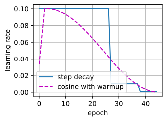
7.6.2.3 Mixup
Mixup (Zhang et al. 2018) builds each training example as a convex combination of two real ones. Draw a mixing weight \(\lambda \sim \mathrm{Beta}(\alpha, \alpha)\) and a random partner for every image in the batch, then train on
\[ \tilde{\mathbf{x}} = \lambda \mathbf{x}_i + (1-\lambda) \mathbf{x}_j, \qquad \tilde{y} = \lambda y_i + (1-\lambda) y_j, \tag{7.6.3}\]
where the mixed label \(\tilde{y}\) is a distribution over classes. Because cross-entropy is linear in the target distribution, training on \(\tilde{y}\) is the same as taking a \(\lambda\)-weighted combination of the two ordinary losses, which is how we implement it: no soft-label plumbing needed. The effect is a strong regularizer: the network is asked to behave linearly between training points, which flattens its decision boundaries and combats the memorization of individual examples. With the usual small \(\alpha\) (around 0.1 to 0.2) the Beta distribution is bathtub-shaped, so most batches are barely mixed and a few are blended heavily.
The implementation is a handful of array operations on the batch, with a single \(\lambda\) shared across it:
def mixup(X, y, alpha):
    """Return a mixed batch, both label sets, and the mixing weight."""
    lam = float(torch.distributions.Beta(alpha, alpha).sample())
    perm = torch.randperm(X.shape[0], device=X.device)
    return lam * X + (1 - lam) * X[perm], y, y[perm], lam
def mixup(X, y, alpha):
"""Return a mixed batch, both label sets, and the mixing weight."""
g1, g2 = tf.random.gamma([], alpha), tf.random.gamma([], alpha)
lam = float(g1 / (g1 + g2)) # Beta(a, a) as a ratio of Gammas
perm = tf.random.shuffle(tf.range(tf.shape(X)[0]))
return (lam * X + (1 - lam) * tf.gather(X, perm),
y, tf.gather(y, perm), lam)def mixup(key, X, y, alpha):
"""Return a mixed batch, both label sets, and the mixing weight."""
key_lam, key_perm = jax.random.split(key)
lam = jax.random.beta(key_lam, alpha, alpha)
perm = jax.random.permutation(key_perm, X.shape[0])
return lam * X + (1 - lam) * X[perm], y, y[perm], lamdef mixup(X, y, alpha):
"""Return a mixed batch, both label sets, and the mixing weight."""
lam = float(np.random.beta(alpha, alpha, size=1)[0])
perm = np.arange(X.shape[0], dtype='int32')
np.random.shuffle(perm)
return lam * X + (1 - lam) * X[perm], y, y[perm], lamTo make the blending visible we mix a batch of Fashion-MNIST images with \(\alpha = 2\), which pulls \(\lambda\) toward the middle of its range instead of the extremes (training uses a much smaller \(\alpha\)); the cell prints the single draw this batch got, so how strongly the images blend varies from run to run. The top row shows the originals, the bottom row their mixtures with a shuffled partner:
data = d2l.FashionMNIST(batch_size=8)
X, y = next(iter(data.train_dataloader()))
X_mix, y_a, y_b, lam = mixup(X, y, alpha=2.0)
d2l.show_images(torch.cat([X, X_mix]).squeeze(1), 2, 8)
print(f'lambda = {float(lam):.2f}')
lambda = 0.90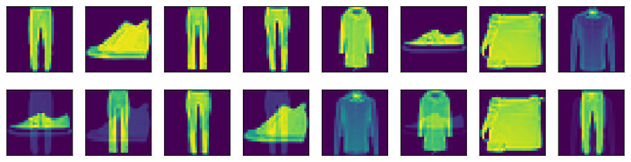
data = d2l.FashionMNIST(batch_size=8)
X, y = next(iter(data.train_dataloader()))
X_mix, y_a, y_b, lam = mixup(X, y, alpha=2.0)
d2l.show_images(tf.squeeze(tf.concat([X, X_mix], axis=0), -1), 2, 8)
print(f'lambda = {lam:.2f}')
lambda = 0.14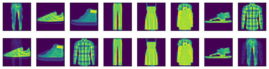
data = d2l.FashionMNIST(batch_size=8)
X, y = next(iter(data.train_dataloader()))
X_mix, y_a, y_b, lam = mixup(d2l.get_key(), jnp.asarray(X),
                             jnp.asarray(y), alpha=2.0)
d2l.show_images(jnp.concatenate([jnp.asarray(X), X_mix]).squeeze(-1), 2, 8)
print(f'lambda = {lam:.2f}')
lambda = 0.41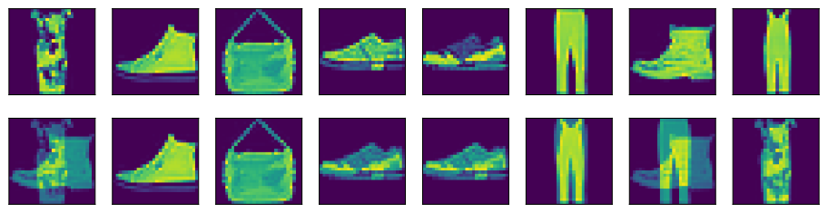
data = d2l.FashionMNIST(batch_size=8)
X, y = next(iter(data.train_dataloader()))
X_mix, y_a, y_b, lam = mixup(X, y, alpha=2.0)
d2l.show_images(np.concatenate([X, X_mix]).squeeze(axis=1), 2, 8)
print(f'lambda = {lam:.2f}')
lambda = 0.52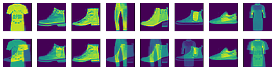
CutMix (Yun et al. 2019) is the spatial sibling: instead of blending two images everywhere, it cuts a rectangular patch from one image and pastes it into the other, mixing the labels in proportion to the patch area. It preserves local image statistics (every pixel comes from a real photograph) and in practice modern recipes alternate randomly between Mixup and CutMix from batch to batch. Its implementation is a rectangle-slicing variant of the code above, which we leave as an exercise.
7.6.2.4 Stochastic Depth
Dropout (Section 4.6) randomly silences individual activations. Stochastic depth (Huang et al. 2016) applies the same idea at the coarsest possible granularity: during training, each residual block’s entire branch is dropped with some probability, so the block passes its input through unchanged and that training step sees a shallower network. Residual connections make this safe, since the identity path is always there to carry the signal. For a residual block computing \(\mathbf{x} + f(\mathbf{x})\), we replace the branch by
\[ \mathbf{x} + \frac{b}{1 - p} f(\mathbf{x}), \qquad b \sim \mathrm{Bernoulli}(1-p), \tag{7.6.4}\]
where the \(1/(1-p)\) rescaling keeps the branch’s expected contribution unchanged, so at evaluation time we use the block without stochastic dropping. Modern implementations draw \(b\) per sample rather than per batch. The wrapper below subclasses the Residual block of Section 7.4 and inserts the drop before the addition; running a large batch through it in training mode confirms that close to a fraction \(p\) of the samples pass through untouched.
def drop_path(Y, p, training):
    if not training or p == 0:
        return Y
    keep = (torch.rand(Y.shape[0], 1, 1, 1, device=Y.device) > p).float()
    return Y * keep / (1 - p)

class StochasticResidual(d2l.Residual):
    """A residual block whose branch is dropped with probability p."""
    def __init__(self, num_channels, p):
        super().__init__(num_channels)
        self.p = p

    def forward(self, X):
        Y = self.bn2(self.conv2(F.relu(self.bn1(self.conv1(X)))))
        return F.relu(drop_path(Y, self.p, self.training) + X)

blk, X = StochasticResidual(3, p=0.5), torch.randn(1000, 3, 8, 8)
blk(X)  # Initialize the lazy layers
blk.train()
dropped = (blk(X) == F.relu(X)).flatten(1).all(1).float().mean()
print(f'fraction of samples with a dropped branch: {float(dropped):.3f}')
fraction of samples with a dropped branch: 0.476def drop_path(Y, p, training):
if not training or p == 0:
return Y
keep = tf.cast(tf.random.uniform((tf.shape(Y)[0], 1, 1, 1)) > p, Y.dtype)
return Y * keep / (1 - p)
class StochasticResidual(d2l.Residual):
"""A residual block whose branch is dropped with probability p."""
def __init__(self, num_channels, p):
super().__init__(num_channels)
self.p = p
def call(self, X, training=False):
Y = tf.keras.activations.relu(self.bn1(self.conv1(X),
training=training))
Y = self.bn2(self.conv2(Y), training=training)
return tf.keras.activations.relu(drop_path(Y, self.p, training) + X)
blk, X = StochasticResidual(3, p=0.5), tf.random.normal((1000, 8, 8, 3))
Y = blk(X, training=True)
diff = tf.reshape(tf.abs(Y - tf.keras.activations.relu(X)), (1000, -1))
dropped = tf.reduce_mean(tf.cast(tf.reduce_max(diff, 1) == 0, tf.float32))
print(f'fraction of samples with a dropped branch: {float(dropped):.3f}')fraction of samples with a dropped branch: 0.523class StochasticResidual(nnx.Module):
"""A residual block with per-sample stochastic depth."""
deterministic: bool
def __init__(self, num_channels, p, rngs=None):
rngs = (nnx.Rngs(params=d2l.get_key(), drop_path=d2l.get_key())
if rngs is None else rngs)
self.p, self.deterministic, self.rngs = p, False, rngs
self.conv1 = nnx.Conv(num_channels, num_channels, (3, 3),
padding='same', rngs=rngs)
self.bn1 = nnx.BatchNorm(num_channels, rngs=rngs)
self.conv2 = nnx.Conv(num_channels, num_channels, (3, 3),
padding='same', rngs=rngs)
self.bn2 = nnx.BatchNorm(num_channels, rngs=rngs)
def set_view(self, *, deterministic):
self.deterministic = deterministic
def __call__(self, X):
Y = self.conv1(X)
Y = nnx.relu(self.bn1(Y))
Y = self.bn2(self.conv2(Y))
if not self.deterministic and self.p > 0:
keep = jax.random.bernoulli(
self.rngs.drop_path(), 1 - self.p,
(X.shape[0], 1, 1, 1))
Y = Y * keep / (1 - self.p)
return nnx.relu(X + Y)
blk = StochasticResidual(3, p=0.5)
X = jax.random.normal(d2l.get_key(), (1000, 8, 8, 3))
Y = blk(X)
dropped = jnp.all(Y == nnx.relu(X), axis=(1, 2, 3)).mean()
print(f'fraction of samples with a dropped branch: {float(dropped):.3f}')fraction of samples with a dropped branch: 0.484def drop_path(Y, p, training):
if not training or p == 0:
return Y
keep = (np.random.uniform(size=(Y.shape[0], 1, 1, 1)) > p).astype(
'float32')
return Y * keep / (1 - p)
class StochasticResidual(d2l.Residual):
"""A residual block whose branch is dropped with probability p."""
def __init__(self, num_channels, p):
super().__init__(num_channels)
self.p = p
def forward(self, X):
Y = self.bn2(self.conv2(npx.relu(self.bn1(self.conv1(X)))))
return npx.relu(drop_path(Y, self.p, autograd.is_training()) + X)
blk, X = StochasticResidual(3, p=0.5), np.random.normal(size=(1000, 3, 8, 8))
blk.initialize()
with autograd.record():
Y = blk(X)
dropped = (np.abs(Y - npx.relu(X)).reshape(1000, -1).max(axis=1) == 0).mean()
print(f'fraction of samples with a dropped branch: {float(dropped):.3f}')fraction of samples with a dropped branch: 0.533In deep networks the drop probability is usually ramped linearly from 0 in the earliest block to a maximum (0.1 to 0.5) in the last. The vectorized per-sample implementation above computes the branch before masking it, so it regularizes but does not save arithmetic. The original per-minibatch method can skip a dropped branch entirely and thereby shorten training.
7.6.2.5 Averaging Weights
The last row of Table 7.6.1 costs almost nothing. Stochastic gradients cause parameters to fluctuate within a low-loss region. Averaging the iterates reduces these fluctuations, an approach also used by stochastic weight averaging (Izmailov et al. 2018). The online version keeps a shadow copy \(\bar{\theta}\) of the parameters and after every update blends in the current weights,
\[ \bar{\theta} \leftarrow \beta \bar{\theta} + (1-\beta) \theta, \tag{7.6.5}\]
with a decay \(\beta\) close to 1 (0.99 to 0.9999). Training uses \(\theta\) as usual; only evaluation uses \(\bar{\theta}\). The class below is the entire mechanism; we exercise it on a deliberately noisy sequence of “weights” to show the variance reduction.
class EMA:
    """A shadow copy of a model's parameters, updated after each step."""
    def __init__(self, model, decay=0.99):
        self.decay = decay
        self.shadow = {k: v.detach().clone()
                       for k, v in model.state_dict().items()}

    def update(self, model):
        for k, v in model.state_dict().items():
            if v.dtype.is_floating_point:
                self.shadow[k].mul_(self.decay).add_(v, alpha=1 - self.decay)
            else:
                self.shadow[k].copy_(v)  # e.g., batch-norm step counters

net = nn.Linear(1, 1, bias=False)
ema, raw, avg = EMA(net, decay=0.9), [], []
for t in range(100):
    with torch.no_grad():  # Simulate noisy SGD iterates around 1.0
        net.weight.copy_(1 + 0.3 * torch.randn(1, 1))
    ema.update(net)
    raw.append(float(net.weight.detach()))
    avg.append(float(ema.shadow['weight']))
d2l.plot(list(range(100)), [raw, avg], xlabel='step', ylabel='weight',
         legend=['raw iterates', 'EMA'])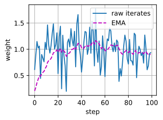
Keras builds this into the optimizer: tf.keras.optimizers.AdamW(..., use_ema=True, ema_momentum=0.99) maintains the shadow weights internally. Its finalize_variable_values method copies the averages into the model variables before evaluation when a custom loop does not finalize them automatically.
Gluon has no built-in weight EMA; the same shadow-dictionary loop as in the PyTorch tab works verbatim over net.collect_params(), blending each parameter’s data() into a kept copy after every trainer.step.
ema_tx = optax.ema(0.9, debias=False)
state = ema_tx.init(jnp.array(0.0))
raw, avg = [], []
for t in range(100):
    value = 1 + 0.3 * jax.random.normal(d2l.get_key(), ())
    averaged, state = ema_tx.update(value, state)
    raw.append(float(value))
    avg.append(float(averaged))
d2l.plot(list(range(100)), [raw, avg], xlabel='step', ylabel='weight',
         legend=['raw iterates', 'EMA'])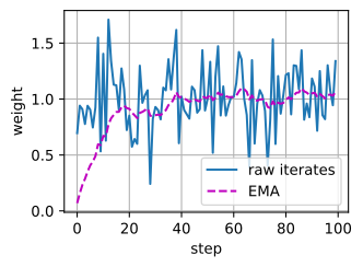
The choice of \(\beta\) sets an averaging horizon of roughly \(1/(1-\beta)\) steps. If that horizon is long relative to the schedule’s tail, the average lags behind the still-improving weights and EMA hurts; matched to the tail, it helps. The exercises ask you to map this trade-off.
7.6.3 Controlled Comparison on One Network
We now combine these ingredients. The network is the ResNet-18 of Section 7.4, rebuilt here from the library’s Residual block. The task is Fashion-MNIST at \(96 \times 96\) resolution, with one deliberate modification: we train on a random subset of 10,000 of the 60,000 training images. This makes regularization consequential without turning the notebook into an ImageNet-scale experiment. You can rerun it at full size by changing one argument, but the comparison would then require retuning both recipes.
class FashionMNIST10k(d2l.FashionMNIST):
    """Fashion-MNIST with the training set subsampled to num_train images."""
    def __init__(self, batch_size=128, resize=(96, 96), num_train=10000):
        super().__init__(batch_size, resize)
        g = torch.Generator().manual_seed(42)  # Same subset for both recipes
        idx = torch.randperm(len(self.train), generator=g)[:num_train]
        self.train = torch.utils.data.Subset(self.train, idx)

class ResNet18(d2l.Classifier):
    """The ResNet-18 of the previous section, built from d2l.Residual."""
    arch = ((2, 64), (2, 128), (2, 256), (2, 512))

    def __init__(self, lr=0.1, num_classes=10):
        super().__init__()
        self.save_hyperparameters()
        layers = [nn.LazyConv2d(64, kernel_size=7, stride=2, padding=3),
                  nn.LazyBatchNorm2d(), nn.ReLU(),
                  nn.MaxPool2d(kernel_size=3, stride=2, padding=1)]
        for i, (num_residuals, c) in enumerate(self.arch):
            for j in range(num_residuals):
                downsample = (j == 0 and i > 0)
                layers.append(d2l.Residual(c, use_1x1conv=downsample,
                                           strides=2 if downsample else 1))
        layers += [nn.AdaptiveAvgPool2d((1, 1)), nn.Flatten(),
                   nn.LazyLinear(num_classes)]
        self.net = nn.Sequential(*layers)

    def lr_at(self, epoch, max_epochs):
        return self.lr  # Constant; recipes override this
class FashionMNIST10k(d2l.FashionMNIST):
"""Fashion-MNIST with a fixed training subset."""
def __init__(self, batch_size=128, resize=(96, 96), num_train=10000):
super().__init__(batch_size, resize)
idx = jax.random.permutation(jax.random.key(42), len(self.train[0]))
idx = idx[:num_train]
self.train = (self.train[0][idx], self.train[1][idx])
class ResNet18(d2l.Classifier):
def __init__(self, lr=0.1, num_classes=10, modern=False,
max_epochs=30, steps_per_epoch=79, rngs=None):
super().__init__()
self.save_hyperparameters(ignore=['rngs'])
rngs = (nnx.Rngs(params=d2l.get_key(), dropout=d2l.get_key(),
mixup=d2l.get_key()) if rngs is None else rngs)
self.rngs = rngs
layers = [nnx.Conv(1, 64, (7, 7), strides=(2, 2), padding='same',
rngs=rngs),
nnx.BatchNorm(64, rngs=rngs), nnx.relu,
lambda x: nnx.max_pool(x, (3, 3), (2, 2), padding='SAME')]
arch = ((2, 64), (2, 128), (2, 256), (2, 512))
in_channels = 64
for i, (depth, c) in enumerate(arch):
for j in range(depth):
down = (i > 0 and j == 0)
layers.append(d2l.Residual(
c, use_1x1conv=down,
strides=(2, 2) if down else (1, 1),
in_channels=in_channels, rngs=rngs))
in_channels = c
layers += [lambda x: x.mean(axis=(1, 2)),
nnx.Linear(512, num_classes, rngs=rngs)]
self.net = nnx.Sequential(*layers)
def configure_optimizers(self):
total = self.max_epochs * self.steps_per_epoch
if self.modern:
schedule = optax.warmup_cosine_decay_schedule(
0.0, self.lr, 3 * self.steps_per_epoch, total)
return optax.adamw(schedule, weight_decay=0.05)
schedule = optax.piecewise_constant_schedule(
self.lr, {int(0.6 * total): 0.1, int(0.85 * total): 0.1})
return optax.sgd(schedule, momentum=0.9)
def training_step(self, batch):
if not self.modern:
return super().training_step(batch)
X, y = batch
X, y_a, y_b, lam = mixup(self.rngs.mixup(), X, y, alpha=0.2)
logp = jax.nn.log_softmax(self(X))
eye = jnp.eye(self.num_classes)
ta = 0.9 * eye[y_a] + 0.1 / self.num_classes
tb = 0.9 * eye[y_b] + 0.1 / self.num_classes
loss_a = -(ta * logp).sum(axis=1).mean()
loss_b = -(tb * logp).sum(axis=1).mean()
return lam * loss_a + (1 - lam) * loss_bThe executable comparison uses a compact subset of the full recipe: optimizer, schedule, label smoothing, Mixup, and duration. It omits RandAugment, CutMix, stochastic depth, and EMA so that the experiment remains small enough to rerun in a textbook notebook. We call it the compact modern recipe below rather than attributing its result to the entire package.
class RecipeTrainer(d2l.Trainer):
    """A Trainer that sets the learning rate from the model's schedule."""
    def fit_epoch(self):
        for group in self.optim.param_groups:
            group['lr'] = self.model.lr_at(self.epoch, self.max_epochs)
        super().fit_epoch()

class ClassicRecipe(ResNet18):
    """Recipe A, ca. 2015: SGD with momentum, step decay, plain loss."""
    def configure_optimizers(self):
        return torch.optim.SGD(self.parameters(), lr=self.lr,
                               momentum=0.9, weight_decay=5e-4)

    def lr_at(self, epoch, max_epochs):
        return step_decay(epoch, max_epochs, self.lr)

class ModernRecipe(ResNet18):
    """Recipe B, ca. 2022: AdamW, cosine warmup, smoothing, Mixup."""
    def configure_optimizers(self):
        return torch.optim.AdamW(self.parameters(), lr=self.lr,
                                 weight_decay=0.05)

    def lr_at(self, epoch, max_epochs):
        return cosine_warmup(epoch, max_epochs, self.lr)

    def loss(self, y_hat, y):
        return F.cross_entropy(y_hat, y, label_smoothing=0.1)

    def training_step(self, batch):
        X, y_a, y_b, lam = mixup(*batch, alpha=0.2)
        y_hat = self(X)
        l = lam * self.loss(y_hat, y_a) + (1 - lam) * self.loss(y_hat, y_b)
        self.plot('loss', l, train=True)
        return l
We give the modern recipe a 1.5x longer budget (45 epochs versus 30), since longer training is itself part of the recipe, and evaluate both on the untouched 10,000-image test set.
def val_accuracy(model, data, trainer):
    model.eval()
    correct, n = 0.0, 0
    with torch.no_grad():
        for X, y in map(trainer.prepare_batch, data.val_dataloader()):
            correct += float(model.accuracy(
                model(X), y, averaged=False).sum())
            n += len(y)
    return correct / n
def val_accuracy(model, data, trainer):
correct, n = 0.0, 0
for X, y in data.val_dataloader():
values = model.accuracy(trainer.val_model(X), y, averaged=False)
correct += float(values.sum())
n += len(y)
return correct / ndata = FashionMNIST10k()
torch.manual_seed(1)
model = ClassicRecipe(lr=0.05)
trainer = RecipeTrainer(max_epochs=30, num_gpus=1)
model.apply_init([next(iter(data.get_dataloader(True)))[0]], d2l.init_cnn)
trainer.fit(model, data)
classic_score = val_accuracy(model, data, trainer)
classic_score0.9027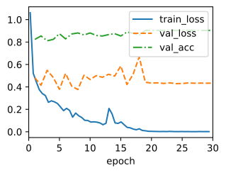
data = FashionMNIST10k()
model = ResNet18(lr=0.05, modern=False, max_epochs=30,
                 steps_per_epoch=len(data.train_dataloader()))
trainer = d2l.Trainer(max_epochs=30, num_gpus=1)
trainer.fit(model, data)
val_accuracy(model, data, trainer)
0.8979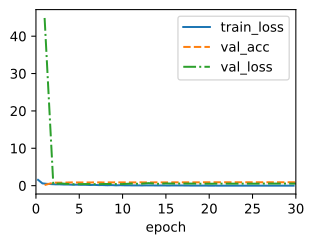
torch.manual_seed(1)
model = ModernRecipe(lr=2e-3)
trainer = RecipeTrainer(max_epochs=45, num_gpus=1)
model.apply_init([next(iter(data.get_dataloader(True)))[0]], d2l.init_cnn)
trainer.fit(model, data)
modern_score = val_accuracy(model, data, trainer)
modern_score
0.9139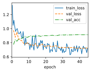
model = ResNet18(lr=2e-3, modern=True, max_epochs=45,
                 steps_per_epoch=len(data.train_dataloader()))
trainer = d2l.Trainer(max_epochs=45, num_gpus=1)
trainer.fit(model, data)
val_accuracy(model, data, trainer)
0.9102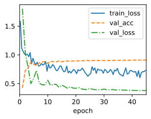
This reduced path demonstrates the optimizer and schedule rather than repeating the full head-to-head run. Keras schedules are objects passed as the learning rate, and the optimizer maintains the weight EMA itself. With 79 batches per epoch, 3 warmup epochs, and a 45-epoch budget:
This reduced path demonstrates the optimizer and schedule rather than repeating the full head-to-head run. MXNet 2.0 registers adamw as an optimizer, and mx.lr_scheduler.CosineScheduler implements warmup followed by cosine decay per step, wired directly into the optimizer. With 79 batches per epoch and a 45-epoch budget:
schedule = tf.keras.optimizers.schedules.CosineDecay(
    initial_learning_rate=0.0, decay_steps=42 * 79,
    warmup_target=2e-3, warmup_steps=3 * 79)
optimizer = tf.keras.optimizers.AdamW(learning_rate=schedule,
                                      weight_decay=0.05,
                                      use_ema=True, ema_momentum=0.99)
[round(float(schedule(step)), 6) for step in (0, 3 * 79, 24 * 79, 45 * 79)]
[0.0, 0.002, 0.001, 0.0]schedule = optax.warmup_cosine_decay_schedule(
init_value=0.0, peak_value=2e-3, warmup_steps=3 * 79,
decay_steps=45 * 79)
optimizer = optax.adamw(learning_rate=schedule, weight_decay=0.05)
[round(float(schedule(step)), 6) for step in (0, 3 * 79, 24 * 79, 45 * 79)][0.0, 0.002, 0.001, 0.0]scheduler = mx.lr_scheduler.CosineScheduler(
max_update=45 * 79, base_lr=2e-3, final_lr=1e-6, warmup_steps=3 * 79)
optimizer = mx.optimizer.AdamW(learning_rate=2e-3, wd=0.05,
lr_scheduler=scheduler)
[round(scheduler(step), 6) for step in (0, 3 * 79, 24 * 79, 45 * 79)][0.0, 0.002, 0.001, 1e-06]Table 7.6.2 reports one seeded run per implementation, rounded to the half point — about the level at which these numbers reproduce from run to run. In both implementations the compact modern recipe gains roughly half a point on the subsampled task; the gain is consistent in direction but modest in size at this scale, and this small teaching experiment is not a substitute for the many-seed ImageNet evaluation of Wightman et al. (2021).
:The same ResNet-18 under both recipes (10,000 Fashion-MNIST training images at \(96 \times 96\); test accuracy, one seeded run each, rounded).
| Implementation | Recipe A (2015, 30 epochs) | Compact modern recipe (45 epochs) |
|---|---|---|
| PyTorch | ≈90.5% | ≈91% |
| JAX | ≈90.5% | ≈91% |
Two practical warnings from this experiment. First, the recipes’ hyperparameters are not interchangeable: recipe A’s learning rate of 0.05 would make AdamW diverge, and recipe B’s rate of 0.002 would starve SGD, so ablating one ingredient requires retuning around it (this is why credible recipe ablations, like those of Wightman et al. (2021), are expensive). Second, the modern recipe’s training loss stays well above recipe A’s, because Mixup and label smoothing make the training targets themselves harder; comparing training losses across recipes tells you nothing about which generalizes better.
7.6.4 Reading the Scoreboard
These results change how reported benchmark numbers, especially on ImageNet, should be interpreted.
First, ImageNet top-1 accuracy separates strong models less clearly than it once did, and the residual differences are heavily recipe-confounded. When an architecture paper reports beating a baseline by a point, the first question is whether both were trained with comparable recipes; as we saw, the recipe alone can change accuracy by four points on a fixed network. Careful papers now retrain baselines under their own recipe. Older cross-paper tables do not support precise conclusions from one-point gaps.
Second, held-out numbers age for more than one reason. When Recht et al. (2019) collected ImageNet-V2 by following the original data-collection protocol (Deng et al. 2009), models lost 11–14 points. The authors found that gains on the original validation set still transferred and attributed the level shift to a slightly harder image distribution rather than adaptive overfitting. A separate problem concerns the labels on the original validation set. Beyer et al. (2020) collected multi-label ReaL annotations and showed that many apparent errors involve ambiguous or multi-object images. ReaL does not relabel ImageNet-V2, so it does not explain away the distribution shift. Together the studies say that both test distribution and annotation protocol matter once model accuracies are close.
Third, the discriminating evaluations have moved downstream. Because ImageNet classification distinguishes leading backbones less clearly than before, backbones are now separated by how well their features transfer: object detection on COCO and semantic segmentation on ADE20K stress resolution, receptive field, and memory behavior in ways a 224-pixel classification task does not, and they reorder models that are indistinguishable on top-1 accuracy. When we evaluate the architectures of the following sections, transfer performance is the score that modern papers argue over.
7.6.5 Summary and Discussion
Between 2015 and the early 2020s, high-accuracy convolutional recipes changed along several axes: many adopted AdamW or LAMB, cosine decay with warmup, stronger augmentation, label smoothing, stochastic depth, longer budgets, and EMA evaluation. These choices are a menu rather than a single standard. In the cited ResNet-50 study their combined effect is about four ImageNet points. Our smaller experiment tests a compact subset of that menu on subsampled Fashion-MNIST and reports its seed-to-seed variation.
That number carries two lessons beyond the ingredients themselves. Methodologically, architecture comparisons require comparable training procedures; a strong baseline retrained with the same methods provides the appropriate control. And practically, if you have a fixed network and a fixed budget, tuning the training procedure can be more economical than changing the architecture. Section 7.7 turns this logic around: starting from the modern recipe, it asks how much of the transformer’s advantage over convnets survives once the recipe is equalized, and modernizes the architecture itself.
7.6.6 Exercises
The comparison on FashionMNIST10k in this section runs in PyTorch and JAX. To work the training problems below in Keras, first assemble the two recipes on the ResNet-18 of Section 7.4 from the pieces this section provides: mixup, CategoricalCrossentropy with label_smoothing, StochasticResidual, and the AdamW optimizer with the CosineDecay schedule from the reduced path. Subsample the training set to 10,000 images with a fixed seed.
The comparison on FashionMNIST10k in this section runs in PyTorch and JAX. To work the training problems below in Gluon, first assemble the two recipes on the ResNet-18 of Section 7.4 from the pieces this section provides: mixup, smoothed_ce, StochasticResidual, and the AdamW optimizer with mx.lr_scheduler.CosineScheduler from the reduced path. Subsample the training set to 10,000 images with a fixed seed.
- [code] Recipe ablation. ● In Table 7.6.2 the compact modern recipe beats recipe A by about half a point, and a single seeded run reproduces only to about the same half point. Whenever a configuration below changes the optimizer, retune the learning rate, since the value that suits AdamW starves SGD.
- Train both recipes on
FashionMNIST10kwith three seeds each and estimate the standard deviation of test accuracy across seeds. How large must the difference between two configurations be before one run of each resolves it? - Starting from the compact modern recipe, replace one ingredient at a time by its recipe A counterpart: remove Mixup, remove label smoothing, replace the warmup and cosine decay of Equation 7.6.2 by recipe A’s step decay, replace AdamW by recipe A’s SGD with momentum, and shorten the budget from 45 to 30 epochs. Which of the five changes in test accuracy exceed the threshold of (a), and do the five add up to the total gap?
- Train the compact modern recipe with both the optimizer and the schedule of recipe A. Together with the compact modern recipe and the optimizer and schedule replacements of (b), this run fills a \(2 \times 2\) table of optimizer against schedule. Do the effects of the two ingredients interact?
- Train both recipes on
- [code] Weight decay and batch normalization. ● The training refinements collected by He et al. (2019) apply weight decay (Section 2.7) only to the weights of convolutional and linear layers and exempt every bias and every scale \(\boldsymbol{\gamma}\) and shift \(\boldsymbol{\beta}\) of batch normalization.
- When batch statistics are used, the output of batch normalization applied to a convolution is unchanged if the convolution’s weights \(\mathbf{W}\) are multiplied by any \(c > 0\). What does weight decay on \(\mathbf{W}\) then do to the loss, to \(\|\mathbf{W}\|\) over the course of training, and to the effective step size of each gradient update?
- Implement both variants, decaying every parameter and decaying only the convolutional and linear weights, on
FashionMNIST10kunder the compact modern recipe. Compare test accuracy and plot the norms of the exempted parameters over training.
- Binary cross-entropy and Mixup. Wightman et al. (2021) train with a binary cross-entropy loss that treats each class as an independent yes/no target. Explain why this loss pairs naturally with Mixup and CutMix. Consider an image that genuinely contains parts of two classes, and contrast how softmax and sigmoid outputs can represent it.
- [code] CutMix. CutMix (Yun et al. 2019) draws \(\lambda\) uniformly from \([0, 1]\), that is, from \(\mathrm{Beta}(1, 1)\) rather than the \(\mathrm{Beta}(0.2, 0.2)\) the compact modern recipe uses for Mixup. It pastes into each image a rectangle from its shuffled partner that covers a fraction \(1 - \lambda\) of the image area. Implement CutMix as a variant of
mixup, and mix the labels as in Equation 7.6.3 with \(\lambda\) replaced by the fraction of the area actually kept, since a rectangle clipped at the image border covers less than \(1 - \lambda\). Train the compact modern recipe onFashionMNIST10konce with CutMix in place of Mixup and once with the two alternating at random from batch to batch, as modern recipes do. Compare the test accuracy of both runs with that of the compact modern recipe, and judge each difference against the half point to which the runs of Table 7.6.2 reproduce. - [code] Stochastic depth in the recipe. ● The compact modern recipe omits stochastic depth. Add it back.
- Extend
StochasticResidualto the downsampling blocks and build the ResNet-18 of Section 7.4 from it, with the drop probability ramped linearly from 0 in the first block to \(p_{\max}\) in the last. What is the expected number of residual branches kept (\(b = 1\)) for one training example, as a function of \(p_{\max}\)? - Sweep \(p_{\max}\) over 0.1, 0.2, and 0.5 on
FashionMNIST10kunder the compact modern recipe, which is itself the case \(p_{\max} = 0\). Does any value raise test accuracy by more than the half point to which the runs of Table 7.6.2 reproduce? How does the best value compare with the range of 0.1 to 0.5 used for much deeper networks? - The per-sample implementation of
StochasticResidualcomputes every branch before masking it. Implement the original per-minibatch variant of Huang et al. (2016), which draws one \(b\) in Equation 7.6.4 per block and step and skips the branch entirely when \(b = 0\). Use (a) to predict the fraction of residual branches it skips at \(p_{\max} = 0.5\). Then measure the fraction of training time it saves and compare the two.
- Extend
- [code] Weight averaging horizon. Add the
EMAclass toModernRecipe: update the shadow copy after every optimizer step and evaluate with the shadow weights. Sweep the decay \(\beta\) of Equation 7.6.5 over 0.9, 0.99, and 0.999. Count the optimizer steps at whichcosine_warmupholds the learning rate below a tenth of its peak, and relate the best decay to that count through the averaging horizon of roughly \(1/(1-\beta)\) steps.
- [code] Weight averaging horizon. Keras optimizers maintain the average themselves: construct
AdamWwithuse_ema=Trueand sweepema_momentum, the decay \(\beta\) of Equation 7.6.5, over 0.9, 0.99, and 0.999. Callfinalize_variable_valuesat the end of training so that the averaged weights are the ones evaluated. Count the optimizer steps at which theCosineDecayschedule holds the learning rate below a tenth of its peak, and relate the best decay to that count through the averaging horizon of roughly \(1/(1-\beta)\) steps.
- [code] Weight averaging horizon. Keep an averaged copy of the parameters with
optax.ema, updated after every optimizer step, and swap it into the model withnnx.updatebefore evaluation. Sweep the decay \(\beta\) of Equation 7.6.5 over 0.9, 0.99, and 0.999. Count the optimizer steps at whichwarmup_cosine_decay_scheduleholds the learning rate below a tenth of its peak, and relate the best decay to that count through the averaging horizon of roughly \(1/(1-\beta)\) steps.
- [code] Weight averaging horizon. Keep a shadow copy of every parameter in
net.collect_params(), blended with the parameter’sdata()after everytrainer.stepas in Equation 7.6.5, and evaluate with the shadow copy. Sweep the decay \(\beta\) over 0.9, 0.99, and 0.999. Count the optimizer steps at whichCosineSchedulerholds the learning rate below a tenth of its peak, and relate the best decay to that count through the averaging horizon of roughly \(1/(1-\beta)\) steps.