from d2l import torch as d2l
import torch
import time
from torch import nn
from torch.nn import functional as F7.5 Efficient ConvNets: Depthwise Separability, Mobile Architectures, and Re-parameterization
The architectures of this chapter so far were designed to win accuracy benchmarks on datacenter GPUs. Many deployment settings instead involve phones, cameras, cars, or embedded boards, where latency, memory, and power matter directly. Efficient convolutional architectures organize this regime around three ideas. First, factorize: replace dense convolutions with the depthwise-separable convolutions of Section 6.4.4. Second, scale and search: once the block is fixed, let optimization allocate widths, depths, and resolutions. Third, re-parameterize: train a multi-branch network, then deploy an algebraically identical single-branch one.
import tensorflow as tf
from d2l import tensorflow as d2l
from d2l import jax as d2l
from flax import nnx
import jax
from jax import numpy as jnp
import optaxfrom d2l import mxnet as d2l
from mxnet import autograd, init, np, npx
from mxnet.gluon import nn
npx.set_np()7.5.1 Depthwise-Separable Networks
7.5.1.1 MobileNet
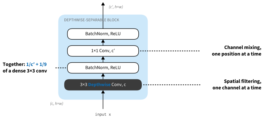
Recall from Section 6.4.4 that a depthwise-separable convolution factorizes a dense \(k \times k\) convolution into a per-channel spatial filter followed by a \(1 \times 1\) channel mixture, cutting parameters and operations to a fraction \(1/c_\textrm{o} + 1/k^2\) of the dense cost (Equation 6.4.1), roughly \(1/9\) for \(3 \times 3\) kernels. In Section 6.4 this was a layer-level observation. MobileNet (Howard et al. 2017) made it an architecture: the entire network is a stack of the block shown in Figure 7.5.1, a depthwise \(3 \times 3\) convolution and a pointwise \(1 \times 1\) convolution, each followed by batch normalization and a ReLU. Downsampling happens inside the block by giving the depthwise convolution a stride of 2, so there are no pooling layers, and a global average pooling head replaces fully connected layers, following NiN (Section 7.2.2). The result matched the ImageNet accuracy of VGG-16 to within a percentage point using roughly \(27\times\) fewer operations and \(33\times\) fewer parameters. A single width multiplier \(\alpha\) scales every channel count in the network, trading accuracy against cost along a smooth curve, so MobileNet is a family in the same sense that VGG is (Section 7.2.1).
7.5.1.2 The Inverted Bottleneck
The bottleneck blocks of ResNet and ResNeXt (Section 7.4.5) compress: a \(1 \times 1\) convolution reduces a wide representation, the \(3 \times 3\) convolution works in the narrow space, and a final \(1 \times 1\) convolution expands it back. This is the right trade when the \(3 \times 3\) convolution is dense and therefore expensive. Once the spatial convolution is depthwise, however, it is cheap even on wide tensors, and the economics reverse. MobileNetV2 (Sandler et al. 2018) therefore inverts the bottleneck: the residual stream stays thin, a \(1 \times 1\) convolution expands it (by a factor of 6 in the paper), the depthwise \(3 \times 3\) convolution operates in the wide expanded space, and a \(1 \times 1\) projection returns to the thin stream. The projection is linear: no ReLU follows it, because a ReLU acting on a low-dimensional representation discards information that cannot be recovered; the paper demonstrates this by ablation. The residual connection joins the thin ends, so the tensors that must be kept in memory across blocks are the small ones. That matters on a phone, where activation memory rather than parameter storage is often the binding constraint.
The inverted bottleneck outlived its mobile origins: ConvNeXt (Section 7.7) adopted the same shape for its blocks, with the depthwise convolution enlarged to \(7 \times 7\) and moved to the front (Liu et al. 2022). We will meet it again when we discuss design spaces in Section 7.8.
7.5.1.3 A Mini-MobileNet
We build a small MobileNetV1-style network for Fashion-MNIST. We use the original block rather than the inverted bottleneck: it is the clearest expression of the factorization, and at Fashion-MNIST scale the difference is negligible. Real mobile networks since MobileNetV2 use inverted bottlenecks throughout. The block below is the pair from Figure 7.5.1; a stride of 2 downsamples.
def dws_block(in_channels, out_channels, stride=1):
    """Depthwise 3x3 and pointwise 1x1 convolutions, each with BN and ReLU."""
    return nn.Sequential(
        nn.Conv2d(in_channels, in_channels, kernel_size=3, stride=stride,
                  padding=1, groups=in_channels, bias=False),
        nn.BatchNorm2d(in_channels), nn.ReLU(),
        nn.Conv2d(in_channels, out_channels, kernel_size=1, bias=False),
        nn.BatchNorm2d(out_channels), nn.ReLU())
class DWSBlock(tf.keras.layers.Layer):
"""Depthwise 3x3 and pointwise 1x1 convolutions, each with BN and ReLU."""
def __init__(self, out_channels, strides=1):
super().__init__()
self.net = tf.keras.models.Sequential([
tf.keras.layers.DepthwiseConv2D(
kernel_size=3, strides=strides, padding='same',
use_bias=False, depthwise_initializer='he_normal'),
tf.keras.layers.BatchNormalization(momentum=0.9),
tf.keras.layers.ReLU(),
tf.keras.layers.Conv2D(out_channels, kernel_size=1,
use_bias=False,
kernel_initializer='he_normal'),
tf.keras.layers.BatchNormalization(momentum=0.9),
tf.keras.layers.ReLU()])
def call(self, X):
return self.net(X)class DWSBlock(nnx.Module):
"""Depthwise 3x3 and pointwise 1x1 convolutions, each with BN and ReLU."""
def __init__(self, in_channels, out_channels, strides=(1, 1), rngs=None):
rngs = nnx.Rngs(d2l.get_key()) if rngs is None else rngs
he = nnx.initializers.he_normal()
self.depthwise = nnx.Conv(
in_channels, in_channels, kernel_size=(3, 3), strides=strides,
padding='same', feature_group_count=in_channels, use_bias=False,
kernel_init=he, rngs=rngs)
self.bn1 = nnx.BatchNorm(in_channels, momentum=0.9, rngs=rngs)
self.pointwise = nnx.Conv(in_channels, out_channels,
kernel_size=(1, 1), use_bias=False,
kernel_init=he, rngs=rngs)
self.bn2 = nnx.BatchNorm(out_channels, momentum=0.9, rngs=rngs)
def __call__(self, X):
X = nnx.relu(self.bn1(self.depthwise(X)))
return nnx.relu(self.bn2(self.pointwise(X)))def dws_block(in_channels, out_channels, strides=1):
"""Depthwise 3x3 and pointwise 1x1 convolutions, each with BN and ReLU."""
blk = nn.Sequential()
blk.add(nn.Conv2D(in_channels, kernel_size=3, strides=strides, padding=1,
groups=in_channels, use_bias=False),
nn.BatchNorm(), nn.Activation('relu'),
nn.Conv2D(out_channels, kernel_size=1, use_bias=False),
nn.BatchNorm(), nn.Activation('relu'))
return blkLike VGG (Section 7.2.1), the whole network is a list of block parameters, here (channels, stride) pairs. A small convolutional stem lifts the grayscale input to 32 channels at half resolution; seven depthwise-separable blocks double the channels while shrinking the feature map; global average pooling and a linear layer produce the class scores.
class MiniMobileNet(d2l.Classifier):
    def __init__(self, arch=((64, 1), (128, 2), (128, 1), (256, 2), (256, 1),
                             (512, 2), (512, 1)),
                 lr=0.1, num_classes=10):
        super().__init__()
        self.save_hyperparameters()
        layers = [nn.Conv2d(1, 32, kernel_size=3, stride=2, padding=1,
                            bias=False),
                  nn.BatchNorm2d(32), nn.ReLU()]
        c = 32
        for c_out, stride in arch:
            layers.append(dws_block(c, c_out, stride))
            c = c_out
        layers += [nn.AdaptiveAvgPool2d((1, 1)), nn.Flatten(),
                   nn.Linear(c, num_classes)]
        self.net = nn.Sequential(*layers)

    def configure_optimizers(self):
        return torch.optim.SGD(self.parameters(), lr=self.lr, momentum=0.9)
class MiniMobileNet(d2l.Classifier):
def __init__(self, arch=((64, 1), (128, 2), (128, 1), (256, 2), (256, 1),
(512, 2), (512, 1)),
lr=0.1, num_classes=10):
super().__init__()
self.save_hyperparameters()
self.net = tf.keras.models.Sequential([
tf.keras.layers.Conv2D(32, kernel_size=3, strides=2,
padding='same', use_bias=False,
kernel_initializer='he_normal'),
tf.keras.layers.BatchNormalization(momentum=0.9),
tf.keras.layers.ReLU()])
for out_channels, strides in arch:
self.net.add(DWSBlock(out_channels, strides))
self.net.add(tf.keras.layers.GlobalAvgPool2D())
self.net.add(tf.keras.layers.Dense(num_classes))
def configure_optimizers(self):
return tf.keras.optimizers.SGD(self.lr, momentum=0.9)class MiniMobileNet(d2l.Classifier):
def __init__(self, arch=((64, 1), (128, 2), (128, 1), (256, 2),
(256, 1), (512, 2), (512, 1)),
lr=0.1, num_classes=10, rngs=None):
super().__init__()
self.save_hyperparameters(ignore=['rngs'])
rngs = nnx.Rngs(d2l.get_key()) if rngs is None else rngs
layers = [nnx.Conv(1, 32, kernel_size=(3, 3), strides=(2, 2),
padding='same', use_bias=False,
kernel_init=nnx.initializers.he_normal(),
rngs=rngs),
nnx.BatchNorm(32, momentum=0.9, rngs=rngs), nnx.relu]
c = 32
for c_out, s in arch:
layers.append(DWSBlock(c, c_out, (s, s), rngs))
c = c_out
layers.extend([lambda x: x.mean(axis=(1, 2)), # global average pooling
nnx.Linear(c, num_classes, rngs=rngs)])
self.net = nnx.Sequential(*layers)
def configure_optimizers(self):
return optax.sgd(self.lr, momentum=0.9)class MiniMobileNet(d2l.Classifier):
def __init__(self, arch=((64, 1), (128, 2), (128, 1), (256, 2), (256, 1),
(512, 2), (512, 1)),
lr=0.1, num_classes=10):
super().__init__()
self.save_hyperparameters()
self.net = nn.Sequential()
self.net.add(nn.Conv2D(32, kernel_size=3, strides=2, padding=1,
use_bias=False),
nn.BatchNorm(), nn.Activation('relu'))
c = 32
for c_out, strides in arch:
self.net.add(dws_block(c, c_out, strides))
c = c_out
self.net.add(nn.GlobalAvgPool2D(), nn.Dense(num_classes))
self.net.initialize(init.Xavier())Before training, let’s verify the arithmetic that motivates the design. The network below has 542,474 trainable parameters. A twin with each depthwise-separable pair replaced by one dense \(3 \times 3\) convolution at the same widths would need \(9 \sum_l c_{\textrm{i},l}\, c_{\textrm{o},l} \approx 4.7\) million parameters in its body, about \(8.8\times\) more, matching the prediction of Equation 6.4.1 for these channel counts.
model = MiniMobileNet()
X = d2l.randn(1, 1, 96, 96)
assert model.net(X).shape == (1, 10)
sum(p.numel() for p in model.parameters())542474model = MiniMobileNet()
X = d2l.normal((1, 96, 96, 1), 0, 1)
assert model.net(X).shape == (1, 10)
sum(int(tf.size(w)) for w in model.net.trainable_weights)542474model = MiniMobileNet()
X = jnp.zeros((1, 96, 96, 1))
assert model(X).shape == (1, 10)
sum(p.size for _, p in nnx.state(model, nnx.Param).flat_state())542474model = MiniMobileNet()
X = d2l.normal(0, 1, (1, 1, 96, 96))
assert model.net(X).shape == (1, 10)
sum(p.data().size for p in model.collect_params().values()
if p.grad_req != 'null')5424747.5.1.4 Training and Comparison
Parameter counts alone do not settle whether the factorization gives anything up, so we train the mini-MobileNet against a plain VGG-style network (Section 7.2.1) at the same parameter budget. Dense \(3 \times 3\) convolutions spend parameters roughly nine times faster per pair of channel counts, so the dense network stops at 128 channels where the separable one reaches 512. Both use batch normalization and an identical global-average-pooling head. The comparison matches parameter count, input resolution, optimizer, and training budget; the separable block and the wider channel allocation it permits change together.
The MXNet path implements and verifies the MobileNet blocks and the RepVGG fusion algebra. It omits this comparative training run, which the other three frameworks each execute independently.
def vgg_stage(num_convs, in_channels, out_channels):
    layers = []
    for _ in range(num_convs):
        layers += [nn.Conv2d(in_channels, out_channels, kernel_size=3,
                             padding=1, bias=False),
                   nn.BatchNorm2d(out_channels), nn.ReLU()]
        in_channels = out_channels
    layers.append(nn.MaxPool2d(2))
    return layers

class VGGSmall(d2l.Classifier):
    """A dense VGG-style network with the same parameter budget."""
    def __init__(self, arch=((2, 32), (2, 64), (2, 128), (2, 128)),
                 lr=0.1, num_classes=10):
        super().__init__()
        self.save_hyperparameters()
        layers, c = [], 1
        for num_convs, c_out in arch:
            layers += vgg_stage(num_convs, c, c_out)
            c = c_out
        layers += [nn.AdaptiveAvgPool2d((1, 1)), nn.Flatten(),
                   nn.Linear(c, num_classes)]
        self.net = nn.Sequential(*layers)

    def configure_optimizers(self):
        return torch.optim.SGD(self.parameters(), lr=self.lr, momentum=0.9)
class VGGSmall(d2l.Classifier):
"""A dense VGG-style network with the same parameter budget."""
def __init__(self, arch=((2, 32), (2, 64), (2, 128), (2, 128)),
lr=0.1, num_classes=10):
super().__init__()
self.save_hyperparameters()
self.net = tf.keras.Sequential()
for num_convs, c_out in arch:
for _ in range(num_convs):
self.net.add(tf.keras.layers.Conv2D(
c_out, 3, padding='same', use_bias=False,
kernel_initializer='he_normal'))
self.net.add(tf.keras.layers.BatchNormalization(momentum=0.9))
self.net.add(tf.keras.layers.ReLU())
self.net.add(tf.keras.layers.MaxPool2D(2))
self.net.add(tf.keras.layers.GlobalAvgPool2D())
self.net.add(tf.keras.layers.Dense(num_classes))
def configure_optimizers(self):
return tf.keras.optimizers.SGD(self.lr, momentum=0.9)class VGGSmall(d2l.Classifier):
"""A dense VGG-style network with the same parameter budget."""
def __init__(self, arch=((2, 32), (2, 64), (2, 128), (2, 128)),
lr=0.1, num_classes=10, rngs=None):
super().__init__()
self.save_hyperparameters(ignore=['rngs'])
rngs = nnx.Rngs(d2l.get_key()) if rngs is None else rngs
layers, c = [], 1
he = nnx.initializers.he_normal()
for num_convs, c_out in arch:
for _ in range(num_convs):
layers += [nnx.Conv(c, c_out, (3, 3), padding='same',
use_bias=False, kernel_init=he,
rngs=rngs),
nnx.BatchNorm(c_out, momentum=0.9, rngs=rngs),
nnx.relu]
c = c_out
layers.append(lambda x: nnx.max_pool(x, (2, 2), (2, 2)))
layers += [lambda x: x.mean(axis=(1, 2)),
nnx.Linear(c, num_classes, rngs=rngs)]
self.net = nnx.Sequential(*layers)
def configure_optimizers(self):
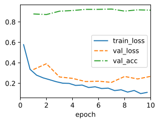
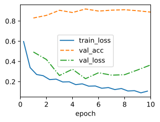
return optax.sgd(self.lr, momentum=0.9)We train both for 10 epochs on Fashion-MNIST at \(96 \times 96\) resolution, with the same trainer and data pipeline we used for ResNet-18 in Section 7.4.
One parity note: Keras’s defaults differ from the other frameworks in two ways that matter at this short budget — Glorot rather than He initialization, and BatchNorm momentum \(0.99\) rather than \(0.9\), whose slowly updated running statistics lag the weights badly after only ten epochs. The models above set both explicitly so that the comparison across framework tabs is like-for-like.
One parity note: Flax NNX’s defaults differ from PyTorch’s in two ways that matter at this short budget — LeCun rather than He initialization, and BatchNorm momentum \(0.99\) rather than \(0.9\), whose slowly updated running statistics lag the weights badly after only ten epochs (they are what evaluation uses). The models above set both explicitly so that the comparison across framework tabs is like-for-like.
data = d2l.FashionMNIST(batch_size=128, resize=(96, 96))

def val_acc(model, data):
    model.eval()
    correct, n = 0.0, 0
    with torch.no_grad():
        for X, y in data.val_dataloader():
            X, y = X.to(d2l.gpu()), y.to(d2l.gpu())
            correct += float(model.accuracy(model(X), y,
                                            averaged=False).sum())
            n += len(y)
    return correct / n

def train_one(model_cls, seed):
    torch.manual_seed(seed)
    model = model_cls(lr=0.05)
    trainer = d2l.Trainer(max_epochs=10, num_gpus=1)
    torch.manual_seed(seed)  # Match minibatch order across the two models
    start = time.perf_counter()
    trainer.fit(model, data)
    return model, val_acc(model, data), (time.perf_counter() - start) / 10
data = d2l.FashionMNIST(batch_size=128, resize=(96, 96))
mobile = MiniMobileNet(lr=0.05)
mobile_trainer = d2l.Trainer(max_epochs=10)
tf.random.set_seed(1)
with d2l.try_gpu():
mobile_trainer.fit(mobile, data)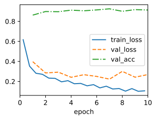
data = d2l.FashionMNIST(batch_size=128, resize=(96, 96))

def train_jax(model_cls, seed):
    d2l.tf.random.set_seed(seed)  # Seed the tf.data shuffle used by JAX
    model = model_cls(lr=0.05, rngs=nnx.Rngs(seed))
    trainer = d2l.Trainer(max_epochs=10, num_gpus=1)
    trainer.fit(model, data)
    correct, n = 0.0, 0
    for X, y in data.val_dataloader():
        values = model.accuracy(trainer.val_model(X), y, averaged=False)
        correct += float(values.sum())
        n += len(y)
return model, trainer, correct / nruns, models = {}, {}
for name, cls in (('mini-MobileNet', MiniMobileNet),
('VGG-style', VGGSmall)):
model, acc, seconds = train_one(cls, seed=1)
models[name] = model
runs[name] = (acc, seconds)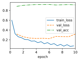
vgg = VGGSmall(lr=0.05)
vgg_trainer = d2l.Trainer(max_epochs=10)
tf.random.set_seed(1)
with d2l.try_gpu():
    vgg_trainer.fit(vgg, data)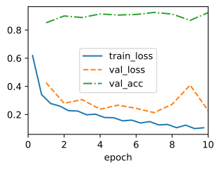
jax_runs, jax_models, jax_trainers = {}, {}, {}
for name, cls in (('mini-MobileNet', MiniMobileNet),
                  ('VGG-style', VGGSmall)):
    model, trainer, acc = train_jax(cls, seed=1)
    jax_models[name], jax_trainers[name] = model, trainer
    jax_runs[name] = acc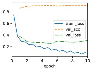
for name, (acc, seconds) in runs.items():
    params = sum(p.numel() for p in models[name].parameters())
    print(f'{name}: {params:,} params, '
          f'val acc {acc:.3f}, {seconds:.1f} s/epoch')
mini-MobileNet: 542,474 params, val acc 0.914, 8.9 s/epoch
VGG-style: 583,594 params, val acc 0.915, 13.6 s/epochdef val_acc(model, data):
correct, n = 0.0, 0
for X, y in data.val_dataloader():
values = model.accuracy(model(X, training=False), y,
averaged=False)
correct += float(tf.reduce_sum(values))
n += len(y)
return correct / n
for name, model in (('mini-MobileNet', mobile), ('VGG-style', vgg)):
count = sum(int(tf.size(w)) for w in model.trainable_variables)
print(f'{name}: {count:,} params, val acc {val_acc(model, data):.3f}')mini-MobileNet: 542,474 params, val acc 0.913
VGG-style: 583,594 params, val acc 0.922for name, acc in jax_runs.items():
model = jax_models[name]
count = sum(p.size for _, p in nnx.state(
model, nnx.Param).flat_state())
print(f'{name}: {count:,} params, val acc {acc:.3f}')mini-MobileNet: 542,474 params, val acc 0.909
VGG-style: 583,594 params, val acc 0.887Table 7.5.1 reports one seeded run per framework; accuracies are rounded to the half point, which is about the level at which they are reproducible from run to run.
:Mini-MobileNet against a dense VGG-style network at matched parameter count (Fashion-MNIST at \(96 \times 96\), 10 epochs; test accuracy, one seeded run per framework, rounded).
| Model | Parameters | Multiply-adds | PyTorch | JAX | TensorFlow |
|---|---|---|---|---|---|
| Mini-MobileNet | 542,474 | 50.3 million | ≈91% | ≈91% | ≈91.5% |
| VGG-style control | 583,594 | 384.9 million | ≈89.5% | ≈89.5% | ≈92.5% |
The two models have comparable accuracy in this small experiment: every run of both architectures falls in a band of roughly 89–93%, and which of the two comes out ahead varies with the framework and the seed — a difference within run-to-run noise, on which no conclusion should be built. The stable result is computational. At this parameter budget the separable network performs about \(7.7\times\) fewer multiply-adds, and its epochs run roughly \(2\)–\(3\times\) faster (in this PyTorch run, about 7 versus 18 seconds). The speedup is far smaller than the operation-count ratio: depthwise convolutions perform little arithmetic per byte of memory, so operation count and wall-clock time diverge. We return to this systems constraint below and in the exercises.
7.5.2 Scaling and Searching
MobileNet fixes a block and picks channel counts by hand. Two further questions remain: how should a network grow when more compute is available, and who chooses the per-stage hyperparameters? EfficientNet (Tan and Le 2019) answered the first with compound scaling. Depth, width, and input resolution all improve accuracy with diminishing returns when scaled alone, so EfficientNet scales them together, multiplying depth by \(\alpha^\phi\), width by \(\beta^\phi\), and resolution by \(\gamma^\phi\) for a single budget knob \(\phi\), with constants fitted once on a small grid subject to \(\alpha \beta^2 \gamma^2 \approx 2\), so that each increment of \(\phi\) doubles the cost. The base network itself was found by neural architecture search over inverted-bottleneck blocks, an automated version of the design-space exploration we study in Section 7.8.
EfficientNetV2 (Tan and Le 2021) revised both halves with training cost in the objective. The search rewards training speed alongside inference speed, and the resulting models replace the depthwise blocks in early, high-resolution stages with dense fused blocks: exactly where depthwise convolutions do too little arithmetic per byte of memory traffic to keep an accelerator busy. Training uses progressive resizing, starting on small images with weak regularization and growing both together, which shortens training severalfold at equal accuracy. FLOP counts favor depthwise convolutions everywhere; measured throughput does not, and the search follows the measurement.
MobileNetV4 (Qin et al. 2024) pushed the same logic across hardware. Its universal inverted bottleneck generalizes the MobileNetV2 block with two optional depthwise convolutions, before the expansion and between expansion and projection; the choices recover the classic inverted bottleneck, a ConvNeXt-like block, a pure feedforward layer, and a new extra-depthwise variant as corners of one searchable space. Searched jointly with a mobile-friendly attention variant, the resulting family is close to Pareto-optimal not on one device but across phone CPUs, DSPs, GPUs, and neural accelerators, whose preferred operations differ. The design lesson of a decade of mobile convnets is that the block is a human insight, but the allocation of width, depth, resolution, and block variant per stage is better treated as an optimization problem against measured latency.
7.5.3 Structural Re-parameterization
7.5.3.1 The RepVGG Block
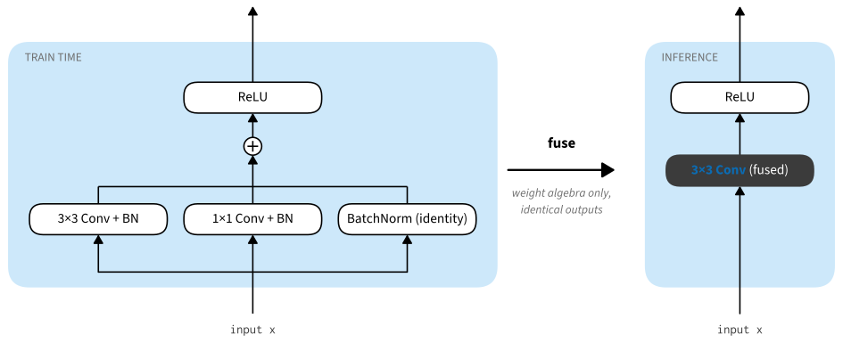
Multi-branch architectures train better than plain ones; that was the lesson of Section 7.4. At inference time, however, every branch must be computed and its output held in memory until the join, and the many small operations of a branchy block leave accelerator kernels underutilized. A VGG-style stack of \(3 \times 3\) convolutions maps efficiently to many inference accelerators: each layer uses one large, regular operation and requires one intermediate activation tensor at a time. RepVGG (Ding et al. 2021) obtains both. During training, each layer is a three-branch block: a \(3 \times 3\) convolution, a \(1 \times 1\) convolution, and an identity path, each with its own batch normalization, summed before the ReLU (Figure 7.5.2). For deployment, the three branches are fused into a single \(3 \times 3\) convolution whose output is identical, not approximately but exactly, because everything involved is linear. The train-time network retains residual-style paths, whereas the deployed network is a plain convolutional stack.
class RepVGGBlock(nn.Module):
    """Train-time block: 3x3, 1x1, and identity branches, each with BN."""
    def __init__(self, num_channels):
        super().__init__()
        self.conv3 = nn.Conv2d(num_channels, num_channels, kernel_size=3,
                               padding=1, bias=False)
        self.conv1 = nn.Conv2d(num_channels, num_channels, kernel_size=1,
                               bias=False)
        self.bn3 = nn.BatchNorm2d(num_channels)
        self.bn1 = nn.BatchNorm2d(num_channels)
        self.bn0 = nn.BatchNorm2d(num_channels)

    def forward(self, X):
        return F.relu(self.bn3(self.conv3(X)) + self.bn1(self.conv1(X))
                      + self.bn0(X))
class RepVGGBlock(tf.keras.Model):
"""Train-time block: 3x3, 1x1, and identity branches, each with BN."""
def __init__(self, num_channels):
super().__init__()
self.conv3 = tf.keras.layers.Conv2D(num_channels, 3, padding='same',
use_bias=False)
self.conv1 = tf.keras.layers.Conv2D(num_channels, 1, use_bias=False)
self.bn3 = tf.keras.layers.BatchNormalization(epsilon=1e-5)
self.bn1 = tf.keras.layers.BatchNormalization(epsilon=1e-5)
self.bn0 = tf.keras.layers.BatchNormalization(epsilon=1e-5)
def call(self, X, training=False):
return tf.keras.activations.relu(
self.bn3(self.conv3(X), training=training)
+ self.bn1(self.conv1(X), training=training)
+ self.bn0(X, training=training))class RepVGGBlock(nnx.Module):
"""Train-time block: 3x3, 1x1, and identity branches, each with BN."""
def __init__(self, num_channels, rngs=None):
rngs = nnx.Rngs(d2l.get_key()) if rngs is None else rngs
self.conv3 = nnx.Conv(num_channels, num_channels, kernel_size=(3, 3),
padding='same', use_bias=False, rngs=rngs)
self.conv1 = nnx.Conv(num_channels, num_channels, kernel_size=(1, 1),
use_bias=False, rngs=rngs)
self.bn3 = nnx.BatchNorm(num_channels, rngs=rngs)
self.bn1 = nnx.BatchNorm(num_channels, rngs=rngs)
self.bn0 = nnx.BatchNorm(num_channels, rngs=rngs)
def __call__(self, X):
return nnx.relu(self.bn3(self.conv3(X)) + self.bn1(self.conv1(X))
+ self.bn0(X))class RepVGGBlock(nn.Block):
"""Train-time block: 3x3, 1x1, and identity branches, each with BN."""
def __init__(self, num_channels):
super().__init__()
self.conv3 = nn.Conv2D(num_channels, kernel_size=3, padding=1,
use_bias=False)
self.conv1 = nn.Conv2D(num_channels, kernel_size=1, use_bias=False)
self.bn3, self.bn1, self.bn0 = (nn.BatchNorm() for _ in range(3))
def forward(self, X):
return npx.relu(self.bn3(self.conv3(X)) + self.bn1(self.conv1(X))
+ self.bn0(X))7.5.3.2 Fusing the Branches
The fusion is three small pieces of weight algebra. At inference time, batch normalization is a fixed affine map per channel: it subtracts the running mean \(\mu_o\), divides by \(\sqrt{\sigma_o^2 + \epsilon}\), scales by \(\gamma_o\), and shifts by \(\beta_o\). Applied to the output of a convolution with kernel \(\mathbf{W}\) and bias \(b_o\), it can be absorbed into a new kernel and bias,
\[ \hat{\mathbf{W}}_o = \frac{\gamma_o}{\sqrt{\sigma_o^2 + \epsilon}}\, \mathbf{W}_o, \qquad \hat{b}_o = \beta_o + \frac{\gamma_o(b_o-\mu_o)}{\sqrt{\sigma_o^2 + \epsilon}}, \tag{7.5.1}\]
where the index \(o\) runs over output channels. The RepVGG convolutions below set \(b_o=0\), giving the shorter expression implemented in fuse_bn. Conv–BN folding is a standard inference optimization for such layer pairs. Next, the two remaining branches are convolutions in disguise. A \(1 \times 1\) kernel is a \(3 \times 3\) kernel that is zero everywhere except at the center, so padding it with a ring of zeros changes nothing. The identity map is a convolution with the kernel \(\mathbf{W}^{\textrm{id}}_{o,i}\) that is 1 at the center position when \(i = o\) and 0 otherwise. Finally, convolution is linear in its kernel: the sum of three convolutions applied to the same input equals one convolution with the summed kernels, and likewise for the biases. Folding each branch by Equation 7.5.1, padding the \(1 \times 1\) kernel, and summing gives the single fused layer.
def fuse_bn(W, bn):
    scale = bn.weight.data / torch.sqrt(bn.running_var + bn.eps)
    return (W * scale.reshape(-1, 1, 1, 1),
            bn.bias.data - bn.running_mean * scale)

def fuse_block(blk):
    c = blk.conv3.weight.shape[0]
    W3, b3 = fuse_bn(blk.conv3.weight.data, blk.bn3)
    W1, b1 = fuse_bn(F.pad(blk.conv1.weight.data, (1, 1, 1, 1)), blk.bn1)
    I = torch.zeros(c, c, 3, 3)
    I[torch.arange(c), torch.arange(c), 1, 1] = 1.0
    W0, b0 = fuse_bn(I, blk.bn0)
    fused = nn.Conv2d(c, c, kernel_size=3, padding=1)
    fused.weight.data, fused.bias.data = W3 + W1 + W0, b3 + b1 + b0
    return fused
def fuse_bn(W, bn):
scale = bn.gamma / tf.sqrt(bn.moving_variance + bn.epsilon)
return W * scale, bn.beta - bn.moving_mean * scale
def fuse_block(blk):
c = blk.conv3.kernel.shape[-1]
pad = [[1, 1], [1, 1], [0, 0], [0, 0]]
W3, b3 = fuse_bn(blk.conv3.kernel, blk.bn3)
W1, b1 = fuse_bn(tf.pad(blk.conv1.kernel, pad), blk.bn1)
I = tf.pad(tf.reshape(tf.eye(c), (1, 1, c, c)), pad)
W0, b0 = fuse_bn(I, blk.bn0)
return W3 + W1 + W0, b3 + b1 + b0def fuse_bn(W, bn, eps=1e-5):
scale = bn.scale[...] / jnp.sqrt(bn.var[...] + eps)
return W * scale, bn.bias[...] - bn.mean[...] * scale
def fuse_block(blk, c):
pad = ((1, 1), (1, 1), (0, 0), (0, 0))
W3, b3 = fuse_bn(blk.conv3.kernel[...], blk.bn3)
W1, b1 = fuse_bn(jnp.pad(blk.conv1.kernel[...], pad), blk.bn1)
I = jnp.pad(jnp.eye(c).reshape(1, 1, c, c), pad)
W0, b0 = fuse_bn(I, blk.bn0)
return W3 + W1 + W0, b3 + b1 + b0def fuse_bn(W, bn, eps=1e-5):
scale = bn.gamma.data() / np.sqrt(bn.running_var.data() + eps)
return (W * scale.reshape(-1, 1, 1, 1),
bn.beta.data() - bn.running_mean.data() * scale)
def fuse_block(blk):
c = blk.conv3.weight.shape[0]
W1 = np.zeros((c, c, 3, 3))
W1[:, :, 1, 1] = blk.conv1.weight.data().reshape(c, c)
I = np.zeros((c, c, 3, 3))
I[:, :, 1, 1] = np.eye(c)
W3, b3 = fuse_bn(blk.conv3.weight.data(), blk.bn3)
W1, b1 = fuse_bn(W1, blk.bn1)
W0, b0 = fuse_bn(I, blk.bn0)
fused = nn.Conv2D(c, kernel_size=3, padding=1)
fused.initialize()
fused(np.zeros((1, c, 3, 3))) # materialize the deferred parameters
fused.weight.data()[:] = W3 + W1 + W0
fused.bias.data()[:] = b3 + b1 + b0
return fusedFusion uses the running statistics, the same ones inference uses, so before checking equivalence we push a few batches through the block in training mode to move those statistics away from their initialization. The check itself feeds fresh data to the train-time block in inference mode and to the fused convolution, and compares.
blk = RepVGGBlock(8)
blk.train()
for _ in range(4):  # populate the BN running statistics
    blk(torch.randn(32, 8, 16, 16))
blk.eval()
fused = fuse_block(blk)
X = torch.randn(32, 8, 16, 16)
with torch.no_grad():
    Y, Y_fused = blk(X), F.relu(fused(X))
assert torch.allclose(Y, Y_fused, atol=1e-5)
float((Y - Y_fused).abs().max())2.384185791015625e-06blk = RepVGGBlock(8)
for _ in range(4): # populate the BN running statistics
blk(tf.random.normal((32, 16, 16, 8)), training=True)
W_fused, b_fused = fuse_block(blk)
X = tf.random.normal((32, 16, 16, 8))
Y = blk(X, training=False)
Y_fused = tf.nn.relu(tf.nn.conv2d(X, W_fused, strides=1,
padding='SAME') + b_fused)
float(tf.reduce_max(tf.abs(Y - Y_fused)))0.0016694068908691406c = 8
blk = RepVGGBlock(c)
train_blk = nnx.view(blk, use_running_average=False)
for _ in range(4): # populate the BN running statistics
X = jax.random.normal(d2l.get_key(), (32, 16, 16, c))
train_blk(X)
W_fused, b_fused = fuse_block(blk, c)
X = jax.random.normal(d2l.get_key(), (32, 16, 16, c))
Y = nnx.view(blk, use_running_average=True)(X)
fused = nnx.Conv(c, c, kernel_size=(3, 3), padding='same',
rngs=nnx.Rngs(0))
fused.kernel[...] = W_fused
fused.bias[...] = b_fused
Y_fused = nnx.relu(fused(X))
float(jnp.abs(Y - Y_fused).max())2.86102294921875e-06blk = RepVGGBlock(8)
blk.initialize()
for _ in range(4): # populate the BN running statistics
with autograd.train_mode():
blk(np.random.normal(size=(32, 8, 16, 16)))
fused = fuse_block(blk)
X = np.random.normal(size=(32, 8, 16, 16))
float(np.abs(blk(X) - npx.relu(fused(X))).max())1.9073486328125e-06The maximum difference is on the order of \(10^{-6}\), single-precision roundoff: the fused convolution is the same function. The parameter saving is modest, about a tenth. The real change is execution shape: one convolution kernel instead of three plus three normalizations and two additions, one live activation tensor instead of three, and no batch normalization at all at inference time.
7.5.3.3 From Paper to Product
Deployment adds a constraint that the fusion algebra does not model. The fused kernel is a sum of branches whose scales, after folding batch normalization into them by Equation 7.5.1, can differ by orders of magnitude, so the summed weights and the activations they produce have wide, poorly centered distributions. Naive post-training INT8 quantization collapses on such distributions, since it represents each tensor with 256 evenly spaced values: a fused RepVGG drops from 75.1% to 40.2% top-1 accuracy on ImageNet, where a plain ResNet loses a fraction of a point. Quantization-aware re-parameterization variants restore the lost accuracy by constraining the branch statistics during training (Chu et al. 2024). This result distinguishes algebraic equivalence in floating-point arithmetic from behavior after quantization: an equivalent FP32 transformation need not preserve accuracy under a fixed INT8 quantization scheme.
The idea has since appeared in deployment-oriented architectures. MobileOne (Vasu et al. 2023b) applies train-time over-parameterization to depthwise-separable blocks and reports sub-millisecond backbone latency on a phone. FastViT (Vasu et al. 2023a) combines re-parameterized convolutional stages with attention after resolution reduction. Training-time auxiliary branches that fold away also appear in large-kernel and hybrid architectures.
7.5.4 Summary and Discussion
Efficiency is a separate design objective with its own architectures and failure modes. Depthwise separability reduces convolutional arithmetic; inverted bottlenecks arrange the factorized operations so that their largest tensors are transient; compound scaling and architecture search allocate computation across width, depth, and resolution; and structural re-parameterization uses different but algebraically equivalent graphs for training and deployment. Arithmetic alone is insufficient: EfficientNetV2 avoids depthwise convolutions in early stages because of memory traffic, and RepVGG obtains better hardware utilization from fewer, larger operations at similar FLOPs.
As of 2026, deployment choices depend on these measured hardware costs. On the cheapest tier, microcontrollers and entry phones, plain depthwise convnets of the MobileNet lineage remain the only thing that fits. Flagship phones run convolution-attention hybrids such as FastViT and MobileNetV4 variants, using convolutions at high resolution and attention where the feature maps are small. Pure vision transformers appear where a dedicated neural accelerator and its memory budget can be assumed, and in the datacenter. Convnets did not become irrelevant to efficient inference; they remain widely used, and hybrid designs concede exactly as much of the network to attention as the hardware can afford. How to navigate such trade-offs systematically, rather than architecture by architecture, is the subject of Section 7.8.
7.5.5 Exercises
The training comparison of Table 7.5.1 runs in PyTorch, TensorFlow, and JAX. To work the training problems below in Gluon, build VGGSmall as four stages of two \(3 \times 3\) convolutions at widths 32, 64, 128, and 128, each followed by batch normalization and a ReLU, with \(2 \times 2\) max-pooling between stages and the global-average-pooling head of MiniMobileNet, and train both networks with d2l.Trainer.
- Cost ratio for larger kernels. Evaluate the cost ratio of Equation 6.4.1 for \(5 \times 5\) and \(7 \times 7\) kernels. For which output-channel counts \(c_\textrm{o}\) does the pointwise term dominate? What does this imply for architectures that enlarge depthwise kernels, such as ConvNeXt (Section 7.7)?
- [code] The inverted bottleneck. ● MobileNetV2 (Sandler et al. 2018) replaces the block of Figure 7.5.1 by an inverted bottleneck: a \(1 \times 1\) expansion by a factor \(t\), a depthwise \(3 \times 3\) convolution, a linear \(1 \times 1\) projection, and a residual connection whenever input and output shapes match.
- Implement the block with \(t = 6\) and replace the blocks of
MiniMobileNetby it, choosing the widths so that the parameter count stays near 542,474. Train it with the setup of Table 7.5.1. Compare its test accuracy with the table and its time per epoch with that ofMiniMobileNeton the same device. - Add a ReLU after the projection. Train the linear and the ReLU variants with three seeds each, and compare the gap in test accuracy with the spread across seeds. Does the paper’s ablation, which favors the linear projection, reproduce at this scale?
- For a \(96 \times 96\) input, tabulate for each block of both networks the number of elements in its input, its output, and its largest internal tensor. Which network needs more activation memory when every tensor is held in full? Show that an inference implementation of the inverted bottleneck never needs to hold a whole expanded tensor, and determine which tensors then set its peak activation memory.
- Implement the block with \(t = 6\) and replace the blocks of
- [code] Width multiplier. Add a width multiplier \(\alpha\) to
MiniMobileNetthat scales every channel count (Howard et al. 2017). Predict how the parameter count and the number of multiply-adds scale with \(\alpha\), and verify your prediction at \(\alpha = 0.5\). - [code] Width versus resolution. ● Lowering the input resolution is a second way to cut multiply-adds. Using the width multiplier of the previous problem, train
MiniMobileNetat \(\alpha = 1\) on \(48 \times 48\) inputs and at \(\alpha = 0.5\) on \(96 \times 96\) inputs, with two seeds each and otherwise the setup of Table 7.5.1. Compare the two networks in multiply-adds, parameter count, and test accuracy. Fashion-MNIST images have \(28 \times 28\) pixels. How does this limit what the comparison says about scaling resolution in EfficientNet (Tan and Le 2019)? - [code] Arithmetic intensity. ●
MiniMobileNetperforms about \(7.7\times\) fewer multiply-adds thanVGGSmallin Table 7.5.1, yet its epochs are only two to three times faster.- Measure the forward-pass time of both networks on a batch of 128 images. Count how many multiply-adds a \(3 \times 3\) depthwise convolution performs per weight and per input activation, compare the counts with those of a dense \(3 \times 3\) convolution, and use them to explain the gap.
- The arithmetic intensity of a layer is its number of multiply-adds divided by the number of elements it touches: weights, input activations, and output activations. For every block of
MiniMobileNet, compute it for the depthwise convolution and for a dense \(3 \times 3\) convolution with the block’s input width, output width, and stride. In which stages is the ratio of the two intensities largest? Compare them with the stages in which EfficientNetV2 (Tan and Le 2021) replaces depthwise blocks by fused dense ones.
- [code] Folding batch normalization. The function
fuse_bnfolds batch normalization into a preceding convolution without a bias, using Equation 7.5.1 with \(b_o = 0\). Extendfuse_bnto a convolution with bias \(b_o\), and verify numerically that the convolution followed by batch normalization in inference mode agrees with the folded convolution. Then switch batch normalization to training mode, feed the same example inside two different minibatches, and explain why no fixed kernel and bias reproduce both outputs. - [code] Normalization before the convolution. ● Let batch normalization come before a \(3 \times 3\) convolution with zero padding of 1, with no nonlinearity in between. Fold it into the kernel and bias of the convolution and compare the folded layer with the original numerically. At which output positions do they disagree, and with what value would the input have to be padded for the fold to be exact?
- [code] Training with RepVGG blocks. ● If the fused RepVGG layer computes the same function, why not train the plain \(3 \times 3\) stack directly?
- Give
RepVGGBlocka stride and an output width. A downsampling block has stride 2 and a new width, so an identity branch cannot match its shape. Such a block keeps only its \(3 \times 3\) and \(1 \times 1\) branches (Ding et al. 2021). Build a small network from these blocks and a plain network that replaces each block by one \(3 \times 3\) convolution of the same width and stride, followed by batch normalization and a ReLU. Train both on Fashion-MNIST and compare the training curves. - Extend
fuse_blockto the downsampling blocks, fuse the trained RepVGG network, and confirm that its test accuracy is unchanged. - Fold the batch normalization of the plain network into its convolutions with
fuse_bn. Then quantize the weights of both deployed networks to eight bits with a symmetric per-tensor scale, \(\hat{w} = s \cdot \mathrm{round}(w / s)\) with \(s = \max |w| / 127\), and compare the accuracy drops. Relate the outcome to the distribution of the fused weights, as Chu et al. (2024) analyze.
- Give