%matplotlib inline
from d2l import torch as d2l
import torch
from torch import nn

torch.set_float32_matmul_precision('high')13.4 Memory and Precision
The preceding sections focused on execution time. This section considers device-memory capacity. Parameters, optimizer states, saved activations, and the minibatch must all fit simultaneously during training. Their sizes can be estimated before execution and compared with runtime measurements.
We study three methods for reducing the limiting allocation. Lower-precision formats reduce tensor size and can increase throughput. Activation checkpointing recomputes selected activations during backpropagation instead of storing them. Gradient accumulation preserves the effect of a larger batch while processing smaller microbatches.
Prerequisites: the format ladder and tensor-core requirement of Section 13.2; the d2l.Benchmark timer of Section 13.1; the AdamW optimizer states of Section 9.6. This section finally discharges the “gradient accumulation, returned to in the performance chapter” promise of Section 9.4.
%matplotlib inline
from d2l import jax as d2l
import jax
from jax import numpy as jnp
import numpy as np
13.4.1 Memory Components of a Training Step
A training step holds four kinds of tensor in memory, and knowing their sizes lets you predict the peak before you run anything (Figure 13.4.1). Let the model have \(P\) parameters.
- Parameters — \(P\) values. In mixed-precision training these are kept in fp32 (4 bytes) as the master copy: \(4P\) bytes.
- Gradients — one per parameter, produced during the backward pass: another \(4P\) bytes.
- Optimizer states — Adam keeps a first and second moment per parameter (Section 9.6), \(2 \times 4P = 8P\) bytes; plain SGD keeps none.
- Activations — every intermediate result the forward pass produces that the backward pass will need. Unlike the first three, this scales with the batch and the depth: roughly \(\textrm{batch} \times \textrm{sequence} \times \textrm{width} \times \textrm{depth}\), and it is usually the term that blows up.
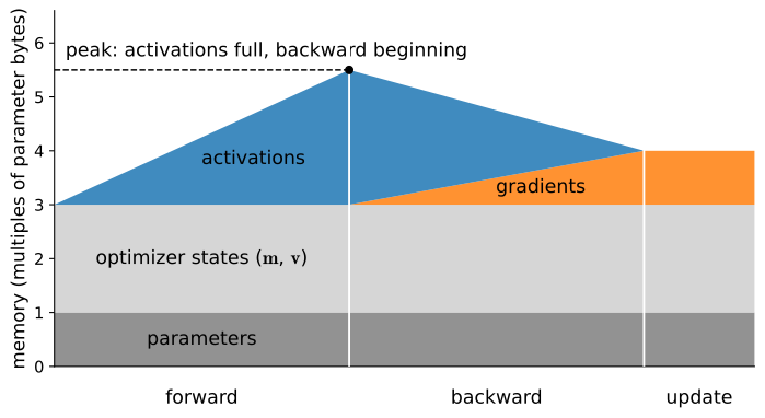
Add the constant terms: training a model with Adam costs about \(4P + 4P + 8P = 16P\) bytes before a single activation — sixteen bytes per parameter, the number to carry in your head. (Mixed precision, below, nudges this to roughly 18–20 by keeping some tensors in two formats; it still saves memory overall, because activations, the dominant term, halve.) The shape of Figure 13.4.1 is the other half of the lesson: activations accumulate through the forward pass and are freed as the backward pass consumes them, so peak memory occurs early in backward — which is exactly the moment activation checkpointing will target.
13.4.2 Measuring Memory
The frameworks expose this memory allocation differently. PyTorch keeps running counters you query at runtime; JAX lets the compiler plan memory ahead of time and reports the plan. Start with PyTorch’s counters, the numbers the anatomy table predicts:
gpu = d2l.try_gpu()
net = nn.Sequential(*[nn.Linear(2048, 2048) for _ in range(6)]).to(gpu)
X = torch.randn(256, 2048, device=gpu)
opt = torch.optim.Adam(net.parameters())

torch.cuda.reset_peak_memory_stats()
opt.zero_grad(set_to_none=True)
net(X).sum().backward()
opt.step()
P = sum(p.numel() for p in net.parameters())
print(f'{P/1e6:.1f}M params  '
      f'predicted states+grads+params: {16 * P / 1e6:.0f} MB')
print(f'measured peak: {torch.cuda.max_memory_allocated() / 1e6:.0f} MB '
      f'allocated, {torch.cuda.max_memory_reserved() / 1e6:.0f} MB reserved')
25.2M params predicted states+grads+params: 403 MB
measured peak: 524 MB allocated, 547 MB reservedThe measured peak overshoots the \(16P\) prediction by roughly 30%, and the gap has an anatomy of its own: this stack’s activations (about 13 MB), autograd bookkeeping and cuBLAS workspaces, temporaries that the fused optimizer update allocates (about the size of one more gradient set), and the caching allocator’s block rounding. The second printed number is larger again: max_memory_allocated counts bytes inside live tensors, while max_memory_reserved is the caching allocator’s high-water mark — the distinction Section 5.7 dissects. So read \(16P\) as this configuration’s floor — fp32 parameters under Adam — rather than as the whole anatomy. Whether activations dominate the total is workload-dependent, decided by batch, sequence length, and depth; in the transformer regime they do.
For a finer picture, PyTorch can record every allocation and free as a snapshot. Rather than embed its interactive viewer, we reconstruct the one plot that matters — allocated bytes over the step — directly from the recorded trace, and see the sawtooth of Figure 13.4.1 in real data:
torch.cuda.memory._record_memory_history(max_entries=100000)
for _ in range(3):
    opt.zero_grad(set_to_none=True)
    net(X).sum().backward()
    opt.step()
snapshot = torch.cuda.memory._snapshot()
torch.cuda.memory._record_memory_history(enabled=None)

# Reconstruct cumulative allocated bytes from the allocation trace.
cum, series = 0, []
for ev in snapshot['device_traces'][0]:
    if ev['action'] == 'alloc':
        cum += ev['size']
    elif ev['action'] == 'free_completed':
        cum -= ev['size']
    series.append(cum / 1e6)
d2l.plot(list(range(len(series))), [series],
         'allocation event', 'allocated (MB)')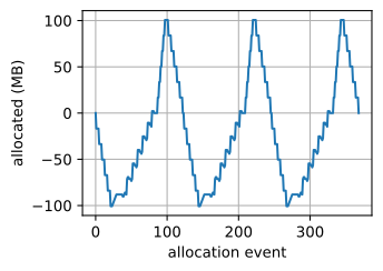
Each cycle is one training step: memory climbs through the forward pass as activations accumulate, then falls through the backward pass as they are released — exactly the anatomy, now measured. The JAX side plans instead of counting. Ahead-of-time compilation (Section 13.3) hands back an object whose memory_analysis() reports what the compiler decided to allocate, before any memory is touched:
def loss_fn(params, X):
    h = X
    for W in params:
        h = jax.nn.relu(h @ W)
    return h.sum()

key = jax.random.PRNGKey(0)
params = [jax.random.normal(k, (2048, 2048)) * 0.02
          for k in jax.random.split(key, 6)]
X = jax.random.normal(key, (256, 2048))

compiled = jax.jit(jax.grad(loss_fn)).lower(params, X).compile()
a = compiled.memory_analysis()
print(f'compiler-planned temp memory: {a.temp_size_in_bytes / 1e6:.0f} MB')
print(f'argument + output: '
      f'{(a.argument_size_in_bytes + a.output_size_in_bytes) / 1e6:.0f} MB')
compiler-planned temp memory: 15 MB
argument + output: 203 MBPyTorch counts allocations as they occur, whereas XLA plans memory at compile time. Neither is better; they reflect the eager-versus-traced split of Section 13.3, and knowing which mental model your framework uses tells you where to look when memory surprises you. Just do not compare the two frameworks’ digits head-to-head: a compiler’s plan is not an allocator’s high-water mark.
13.4.3 Mixed Precision
The format comparison in Section 13.2 shows that narrower formats can increase supported tensor-core throughput and reduce stored bytes. Mixed precision applies these effects selectively during training: run the compute-heavy operations (matmuls, convolutions) in bf16, where tensor cores are fastest and activations are half-size, while keeping a few numerically delicate things (the master weights, the loss reduction) in fp32. On our Ada card the arithmetic win is real and robust — but only if you know what your baseline is running, the lesson Section 13.2 flagged. Whether plain fp32 matmuls use the tensor cores’ tf32 path is a framework default: PyTorch ships with tf32 off, so an fp32 baseline that leaves tf32 disabled understates baseline throughput and overstates the apparent speedup; JAX on this card runs tf32-class dot compute by default, so its naive baseline is already fair — but is not the true fp32 it appears to be. We time all three configurations, once, so the difference is unmistakable:
net = nn.Sequential(nn.Flatten(),
                    nn.Linear(64 * 64, 8192), nn.ReLU(),
                    nn.Linear(8192, 8192), nn.ReLU(),
                    nn.Linear(8192, 10)).to(gpu)
X = torch.randn(2048, 1, 64, 64, device=gpu)
y = torch.randint(0, 10, (2048,), device=gpu)
opt = torch.optim.SGD(net.parameters(), lr=0.01)
loss = nn.CrossEntropyLoss()

def step(autocast, dtype=None):
    opt.zero_grad(set_to_none=True)
    if autocast:
        with torch.autocast('cuda', dtype=dtype):
            l = loss(net(X), y)
    else:
        l = loss(net(X), y)
    l.backward(); opt.step()

torch.set_float32_matmul_precision('highest')  # Unfair baseline: tf32 off
print(d2l.Benchmark(lambda: step(False), desc='fp32 (tf32 off)'))
torch.set_float32_matmul_precision('high')     # Fair baseline: tf32 on
print(d2l.Benchmark(lambda: step(False), desc='tf32'))
print(d2l.Benchmark(lambda: step(True, torch.bfloat16), desc='bf16 autocast'))
fp32 (tf32 off): 22.58 ms/call
tf32: 17.79 ms/call
bf16 autocast: 9.78 ms/calldef net_fn(params, X, dtype):
h = X.reshape(X.shape[0], -1).astype(dtype)
for W in params[:-1]:
h = jax.nn.relu(h @ W.astype(dtype))
return h @ params[-1].astype(dtype)
key = jax.random.PRNGKey(0)
sizes = [(64 * 64, 8192), (8192, 8192), (8192, 10)]
params = [jax.random.normal(k, s) * 0.02
for k, s in zip(jax.random.split(key, 3), sizes)]
X = jax.random.normal(key, (2048, 64 * 64))
def loss_fn(params, dtype):
return (net_fn(params, X, dtype) ** 2).sum()
grad_fn = jax.jit(jax.grad(loss_fn), static_argnums=1)
with jax.default_matmul_precision('highest'): # Unfair baseline: tf32 off
print(d2l.Benchmark(lambda: grad_fn(params, jnp.float32),
desc='fp32 (tf32 off)'))
# The default on this card is tf32-class compute -- the fair baseline
print(d2l.Benchmark(lambda: grad_fn(params, jnp.float32), desc='tf32'))
print(d2l.Benchmark(lambda: grad_fn(params, jnp.bfloat16), desc='bf16'))fp32 (tf32 off): 26.41 ms/call
tf32: 15.99 ms/call
bf16: 8.70 ms/callAgainst the fair tf32 baseline, bf16 runs about one and a half to two times as fast here — the exact ratio is framework- and shape-dependent — and the three timings show the same two-step effect in both tabs: moving true fp32 dots onto the tf32 tensor cores already yields a sizable change, and bf16 then adds at least as much again. Both are genuine tensor-core wins, not measurement artifacts. Note what the PyTorch tab does not use: a GradScaler. Loss scaling exists to keep tiny fp16 gradients from underflowing fp16’s narrow 5-bit-exponent range; bf16 shares fp32’s 8-bit exponent (Figure 13.2.5), so its gradients do not underflow and no scaler is needed. fp16 with GradScaler remains relevant for pre-Ampere hardware and is examined in an exercise. The JAX tab shows that precision is explicit: dtypes are passed through the computation, and jax.default_matmul_precision sets how fp32 dots are computed (true fp32 versus tf32-class tensor-core compute) without changing what any tensor stores. On this card JAX’s default matches 'high', tf32-class, bit for bit — which is why the middle timing is the fair baseline. PyTorch decides per-operation what to cast; JAX makes you say it. Both land on the same design point: bf16 halves the bytes and doubles the tensor-core rate.
13.4.4 Activation Checkpointing
Mixed precision halves activation memory; activation checkpointing can cut it much further, by refusing to store most activations at all. Recall from Figure 13.4.1 that activations are held from the moment the forward pass produces them until the backward pass consumes them — that storage is the peak. Checkpointing makes a different trade: store only a few activations (at block boundaries), and when the backward pass needs the ones in between, recompute them by re-running that block’s forward pass. This adds recomputation — at most one extra forward pass — to avoid holding a large fraction of the activations; the cells below measure both sides of the trade. This is the same “recompute rather than store” argument the Mamba kernel of Section 12.3 made one level down in the hardware (Chen et al. 2016).
from torch.utils.checkpoint import checkpoint

class Block(nn.Module):
    def __init__(self, d=1024):
        super().__init__()
        self.net = nn.Sequential(nn.Linear(d, d), nn.GELU(), nn.Linear(d, d))
    def forward(self, x):
        return x + self.net(x)

blocks = nn.ModuleList([Block().to(gpu) for _ in range(16)])
X = torch.randn(16384, 1024, device=gpu, requires_grad=True)

def run(use_ckpt):
    h = X
    for blk in blocks:
        # use_reentrant=False is the modern, mandatory-since-2.9 form
        h = checkpoint(blk, h, use_reentrant=False) if use_ckpt else blk(h)
    return h.sum()

for use_ckpt in (False, True):
    for p in blocks.parameters():  # clear grads so the peaks are comparable
        p.grad = None
    X.grad = None
    torch.cuda.reset_peak_memory_stats()
    run(use_ckpt).backward()
    peak = torch.cuda.max_memory_allocated() / 1e6
    t = d2l.Benchmark(lambda: run(use_ckpt).backward()).time
    tag = 'checkpointed' if use_ckpt else 'store all'
    print(f'{tag}: peak {peak:.0f} MB, fwd+bwd {1000 * t:.1f} ms')
store all: peak 4318 MB, fwd+bwd 59.9 ms
checkpointed: peak 2306 MB, fwd+bwd 71.1 msdef block(W1, W2, x):
return x + jax.nn.gelu(x @ W1) @ W2
key = jax.random.PRNGKey(1)
ks = jax.random.split(key, 32) # one key per weight matrix
Ws = [(jax.random.normal(ks[2 * i], (1024, 1024)) * 0.02,
jax.random.normal(ks[2 * i + 1], (1024, 1024)) * 0.02)
for i in range(16)]
X = jax.random.normal(key, (16384, 1024))
# jax.checkpoint (a.k.a. remat) recomputes the block in the backward pass.
ckpt_block = jax.checkpoint(block)
def forward(Ws, X, blk):
h = X
for W1, W2 in Ws:
h = blk(W1, W2, h)
return (h ** 2).sum()
for name, blk in [('store all', block), ('checkpointed', ckpt_block)]:
compiled = jax.jit(jax.grad(forward), static_argnums=2).lower(
Ws, X, blk).compile()
mb = compiled.memory_analysis().temp_size_in_bytes / 1e6
t = d2l.Benchmark(lambda: compiled(Ws, X)).time
print(f'{name}: compiler temp {mb:.0f} MB, fwd+bwd {1000 * t:.1f} ms')store all: compiler temp 3230 MB, fwd+bwd 50.5 ms
checkpointed: compiler temp 1216 MB, fwd+bwd 58.7 msCheckpointing releases about 2 GB of held activations on this 16-block stack — the measured peak falls by nearly half in the allocator’s count and by more than half in the compiler’s plan — and the completion-timed step runs only about 15–20% longer, comfortably under the one-extra-forward bound, since the backward pass dominates the step. It is a trade you make when memory is the binding constraint: checkpointing normally costs time, and its purpose is memory (the rare configurations where recomputation beats a cache-hostile stash do not change the rule). JAX exposes the same mechanism as jax.checkpoint (equivalently jax.remat), with a nicer knob: policies like checkpoint_dots let you say which intermediates to keep, and jax.remat’s companion tools let you watch what was saved — the introspection theme JAX does uniquely well. The trade is identical; the interface reflects each framework’s temperament, imperative versus declarative.
13.4.5 Gradient Accumulation
The final technique buys the statistical effect of a large batch without its memory cost — and discharges a promise made all the way back in Section 9.4. A large batch improves gradient estimates and tensor-core utilization (its intensity is higher, Section 13.1), but a large batch’s activations may not fit. Gradient accumulation splits the desired global batch into \(k\) micro-batches, runs forward and backward on each while summing the gradients, and only then takes one optimizer step. The activations of just one micro-batch are live at a time, so peak memory follows the micro-batch, while the update sees the full global batch: \(B_{\textrm{global}} = B_{\textrm{micro}} \times k\) (times the number of devices, once Section 13.5 adds them). Correctness requires accumulation over \(k\) micro-batches to match one full-batch step, which the following parity check verifies.
net = nn.Linear(1024, 1).to(gpu)
X = torch.randn(128, 1024, device=gpu)
y = torch.randn(128, 1, device=gpu)
loss = nn.MSELoss()

# Full batch: one backward over all 128 rows.
net.zero_grad()
loss(net(X), y).backward()
full = net.weight.grad.clone()

# Accumulated: 4 micro-batches of 32, gradients summed, scaled by 1/4.
net.zero_grad()
for i in range(4):
    xb, yb = X[i * 32:(i + 1) * 32], y[i * 32:(i + 1) * 32]
    (loss(net(xb), yb) / 4).backward()   # /4 because MSE already averages
accumulated = net.weight.grad.clone()
print(f'max gradient difference: {(full - accumulated).abs().max():.2e}')
max gradient difference: 1.19e-07W = jax.random.normal(jax.random.PRNGKey(0), (1024, 1))
X = jax.random.normal(jax.random.PRNGKey(1), (128, 1024))
y = jax.random.normal(jax.random.PRNGKey(2), (128, 1))
def mse(W, X, y):
return ((X @ W - y) ** 2).mean()
full = jax.grad(mse)(W, X, y)
acc = sum(jax.grad(mse)(W, X[i * 32:(i + 1) * 32], y[i * 32:(i + 1) * 32])
for i in range(4)) / 4
print(f'max gradient difference: {jnp.abs(full - acc).max():.2e}')max gradient difference: 3.10e-06The gradients match to floating-point noise. The one subtlety is the averaging: if your loss already averages over the batch (as MSE and cross-entropy do), each micro-batch gradient must be scaled by \(1/k\) so the sum reproduces the mean. The equivalence also rests on conditions this tiny example satisfies silently: an additive per-example loss, equal-size micro-batches (or a properly weighted mean), the same dropout and RNG draws, no batch-coupled state such as BatchNorm — whose statistics would be computed per micro-batch — and clipping or optimizer steps applied only at the global boundary. Accumulation is the right tool when you are memory-bound and want a bigger effective batch; it is the wrong tool when you want to go faster: the arithmetic is identical but arrives as more launches over smaller, lower-intensity GEMMs, so by this chapter’s own accounting it is usually slightly slower — it only rearranges when the optimizer step happens.
13.4.6 Choosing a Memory Optimization
When a model does not fit or runs too slowly, consider the following interventions in increasing order of cost:
- It’s slow, bandwidth- or overhead-bound → compile it (Section 13.3). Usually free.
- It’s slow, compute-bound, or it’s tight on memory → drop to bf16 (mixed precision). Around \(1.5\)–\(2\times\) speed and half the activation bytes.
- It still doesn’t fit → checkpoint activations. Large memory saving for a modest increase in time.
- It still doesn’t fit, and you want a bigger effective batch → accumulate gradients. Bigger effective batch at micro-batch memory — about the same wall-clock, never faster.
- It’s still too slow, or genuinely too big for one card → add devices (Section 13.5).
The next section analyzes the additional accounting required when devices are added.
13.4.7 Summary
- A training step’s memory is parameters (\(4P\)) + gradients (\(4P\)) + optimizer states (Adam: \(8P\)) + activations (batch × depth × width, the term that explodes). About \(16P\) bytes before activations; peak lands early in the backward pass.
- PyTorch measures memory with runtime counters and allocation snapshots; JAX reports the compiler’s ahead-of-time memory plan. Counting versus planning — the eager-versus-traced split again.
- Mixed-precision bf16 raises tensor-core throughput (1.5–2× over a fair tf32 baseline here, framework- and shape-dependent) and halves activation bytes; measure it against that fair tf32 baseline — the frameworks’ fp32 defaults differ — and skip the
GradScaler(bf16 shares fp32’s exponent range — only fp16 needs loss scaling). - Activation checkpointing recomputes instead of stores: peak memory cut roughly in half or better on a deep stack (about 2 GB of activations released) for about 15–20% more step time here. It normally costs time; its purpose is memory — use it when memory binds.
- Gradient accumulation reaches a large effective batch at micro-batch memory cost — \(B_{\textrm{global}} = B_{\textrm{micro}} \times k\) — at the same wall-clock; scale per-micro-batch losses by \(1/k\) when the loss already averages.
13.4.8 Exercises
- Where the peak lands. Figure 13.4.1 places the peak of a training step early in the backward pass. Consider a stack of \(n\) identical layers. The parameters of each layer occupy \(w\) bytes, and its forward pass stores \(a\) bytes of activations. Assume that no gradients exist when the backward pass starts, and that the backward pass of a layer frees the activations of that layer and creates its parameter gradient of \(w\) bytes. Leave out the parameters and the optimizer states, whose sizes stay constant.
- Write the bytes held by activations and gradients after the backward pass has processed \(j\) of the \(n\) layers. Show that the peak lies at the start of the backward pass when \(a > w\) and at its end when \(a < w\).
- Count as activations only the input of each linear layer, and ignore the biases. Which of the two cases holds for the six-layer stack of Section 13.4.2 at its batch size of 256, and at which batch size does the stack switch to the other case?
- Under gradient accumulation over \(k\) micro-batches, the gradients of the first micro-batch stay allocated while the later micro-batches run. Find the peak with accumulation, and the values of \(k\) for which accumulation lowers the peak below that of a single step on the full batch.
- [code] Second copy of the weights. ● Mixed precision keeps some tensors in two formats (Section 13.4.1), and its memory saving rests on the activations being the dominant term.
- For the network of Section 13.4.3 at its batch size of 2048, list the tensors that the backward pass keeps in the tf32 configuration and in the bf16 configuration. Decide for each 16-bit copy of a weight matrix whether the backward pass needs it. Predict which configuration has the higher peak, and find the batch size above which the bf16 configuration has the lower one.
- Measure the peak of the computation that Section 13.4.3 times, in both configurations and at batch sizes 2048 and 16384, and compare the measurements with your predictions.
- A model with \(P = 1.3 \times 10^9\) parameters is trained with AdamW on a card with \(24 \times 10^9\) bytes of memory. Compare the memory left for activations under fp32 training, at \(16P\) bytes, and under mixed precision, at \(18P\) bytes. Name two changes to the optimizer or to the storage formats that leave more room for activations, and state what each change gives up.
- Checkpoint placement. ● Consider a stack of \(n\) identical residual blocks, and measure memory in units of the input of one block. The backward pass of one block needs \(c\) units of stored tensors, its input included. A schedule with segments of \(s\) consecutive blocks stores only the input of each segment during the forward pass. During the backward pass it recomputes one segment at a time, while the stored inputs of the earlier segments remain in memory.
- Derive the peak activation memory as a function of \(s\), and the \(s\) that minimizes it. Count \(c\) for the block of Section 13.4.4, which applies a linear layer, a GELU, and a second linear layer on a residual connection. For its 16 blocks, compare storing everything, the per-block checkpointing of that subsection, and the best segment length. Check the saving of per-block checkpointing against the roughly 2 GB that the subsection reports.
- Chen et al. (2016) reduce the memory further by recursion. The schedule stores the input of the stack and the input of its second half, processes the second half recursively, and then processes the first half recursively from its stored input. For \(n\) a power of two, derive the peak memory and the total number of block forward evaluations, the original forward pass included. For \(n = 16\) and \(n = 1024\), compare both quantities with those of the best segment length.
- [code] Recomputation overhead. Section 13.4.4 bounds the extra work of per-block checkpointing by one forward pass, and it measures about 15–20% more step time on its 16-block stack.
- Suppose that a backward pass costs twice the FLOPs of the corresponding forward pass and that time is proportional to FLOPs. Predict the time overhead if the recomputation repeats the whole forward pass of every block.
- Time the forward pass of the stack alone and its forward-plus-backward step without checkpointing, and predict the overhead again from the two measured times. Compare both predictions with the measured overhead.
- List the tensors that the backward pass of one block reads, and the operations of the block that are needed to recompute them. Predict the overhead from this count, and explain the measured overhead.
- Clipping under accumulation. Gradient clipping to norm \(\tau\) replaces a gradient \(\mathbf{g}\) by \(\mathbf{g} \min(1, \tau / \|\mathbf{g}\|)\). Let \(\mathbf{g}_1, \ldots, \mathbf{g}_k\) be the micro-batch gradients after the scaling by \(1/k\) of Section 13.4.5, so that their sum \(\mathbf{g}\) is the full-batch gradient.
- A training loop clips each \(\mathbf{g}_i\) before adding it to the accumulator. Find the largest norm that the accumulated gradient can reach, and a condition under which the loop gives the same result as clipping \(\mathbf{g}\) once before the optimizer step.
- Under fp16 loss scaling with factor \(S\), the accumulator holds \(S \mathbf{g}\) once the last micro-batch has been added. In which order must the loop divide by \(S\), clip, and step? What goes wrong if it clips before dividing, and what goes wrong if \(S\) changes before the last micro-batch has been added?
- [code] Cost of accumulation. ● Split the global batch of 2048 examples of the bf16 configuration of Section 13.4.3 into \(k\) equal micro-batches, and accumulate their gradients, for \(k = 1, 2, 4, \ldots, 64\).
- Let the network have \(P\) parameters. A micro-batch of \(B_{\textrm{micro}}\) examples performs about \(6 P B_{\textrm{micro}}\) FLOPs in its forward and backward passes, and it moves at least \(12P\) bytes: it reads the bf16 weights in each of the two passes, and it reads and writes the fp32 gradient accumulator. Ignore the activations. Write the peak compute of Equation 13.1.2 as \(F\) here, because \(P\) counts parameters, and take \(F\) and \(\beta\) from the RTX 4090 column of Table 13.2.1. Predict the time per global batch as a function of \(k\), and find the \(k\) beyond which the micro-batches are bandwidth-bound.
- Measure the time per global batch for every \(k\), and plot it together with the prediction. Identify the weight and gradient traffic of the bf16 configuration that the count of \(12P\) bytes leaves out.
- Suppose that activation checkpointing let each micro-batch hold four times as many examples, at the price of a third more FLOPs. Under the model of the first sub-problem, for which \(k \geq 4\) of the sweep does accumulation over \(k/4\) checkpointed micro-batches take less time than accumulation over \(k\) plain ones?
- [extended] GPT-2 on one card. ● The GPT-2 configuration of Section 11.2.4 has width \(d = 768\), 12 blocks with \(n_h = 12\) attention heads, a vocabulary of \(V = 50{,}257\) tokens, and \(P = 124.4\) million parameters. It is trained with AdamW on sequences of \(T = 1024\) tokens, on a card with \(24 \times 10^9\) bytes of memory. Following the count of Korthikanti et al. (2022), a block without dropout stores \(16d\) values per token, and an attention that materializes its score matrices stores another \(n_h T\) values per token. These values take 4 bytes each in fp32 training and 2 bytes each under mixed precision. In both regimes the cross-entropy loss stores the logits as \(V\) fp32 values per token.
- Compute the activation bytes per sequence of the 12 blocks, with a fused and with a materializing attention, in both regimes, and the bytes per sequence of the logits. Korthikanti et al. neglect the logits for models with tens of billions of parameters. What share of the activations do the logits take here, with a fused attention?
- Take \(16P\) persistent bytes for fp32 training and \(18P\) for mixed precision, and assume a fused attention. Predict the largest micro-batch, in sequences, for fp32 training, for mixed precision, and for mixed precision with per-block checkpointing. Per-block checkpointing keeps \(d\) values per token for each block, plus the activations of one block during its recomputation. Which term limits the last configuration?
- Build
GPTin this configuration with random weights, and measure the peak memory of fp32 training steps at micro-batches of 2, 4, and 8 sequences. Fit the peak as a linear function of the micro-batch. At the start of the backward pass, the cross-entropy creates logits-sized gradients while the stored logits are still allocated. Count them for your training step, and add them to the bytes per sequence of the first sub-problem. Compare the slope with this count and the intercept with \(16P\), and decide whether the attention stores its score matrices. - Compute the output head and the loss in chunks of tokens, and checkpoint each chunk so that the logits of only one chunk exist at a time. With per-block checkpointing in both runs, find the largest fp32 micro-batch with the chunked loss and with the unchunked loss. For each run, split a global batch of 512 sequences into equal micro-batches no larger than its largest one, and measure the tokens per second of both schedules.
- [code] Optimizer-step memory. Section 13.4.2 attributes part of the 30% gap between the measured peak and \(16P\) to temporaries of the optimizer update. Rebuild
net,X, andoptof that subsection three times: withtorch.optim.Adam(net.parameters(), foreach=False), with the default arguments, and withfused=True.- Run two training steps with each optimizer. On the second step, record
torch.cuda.memory_allocated()just beforeopt.step(), reset the peak statistics, and recordtorch.cuda.max_memory_allocated()afteropt.step(). Express the extra bytes of each update in units of the gradient size \(4P\). - The three implementations update one parameter tensor at a time, apply each elementwise operation to all parameter tensors at once, or run the whole update in one kernel per group of tensors. Explain the three measurements from this difference, and state which part of the 30% gap they account for.
- Run two training steps with each optimizer. On the second step, record
- [code] fp16 gradient window. ● The 5-bit exponent of fp16
(Figure 13.2.5) gives it normal numbers from \(2^{-14}\) to 65,504 and subnormal numbers down to \(2^{-24}\). Loss scaling (Micikevicius et al. 2018) multiplies the loss by a factor \(S\) before the backward pass and divides the gradients by \(S\) afterwards. Use
net,X,y, andlossas defined in Section 13.4.3, and take as reference the fp32 parameter gradients computed undertorch.set_float32_matmul_precision('highest').- Plot a histogram of \(\log_2 |g|\) over the nonzero entries \(g\) of the reference gradients. Which fractions of the entries lie below \(2^{-14}\) and below \(2^{-24}\), and which factors \(S\) place 99.9% of the scaled entries \(S g\) in the normal range of fp16?
- For \(S = 2^0, 2^2, \ldots, 2^{24}\), compute the gradients of \(S\) times the loss under
torch.autocast('cuda', dtype=torch.float16), divide them by \(S\), and plot their relative error \(\|\hat{\mathbf{g}} - \mathbf{g}\| / \|\mathbf{g}\|\) with respect to the reference \(\mathbf{g}\), marking the runs with non-finite entries. Repeat the sweep withtorch.bfloat16. In which range of \(S\) is fp16 more accurate than bf16, and why is that possible? torch.amp.GradScalerstarts at \(S = 2^{16}\). Where does this factor lie in the window of the previous sub-problem? The gradient of the loss with respect to a logit is the difference between the predicted and the target probability, divided by the batch size of- How does the window move if the batch grows to 32,768 examples? Explain why a static loss scale that works for one workload can fail for another.
- [code] Selective recomputation. ● Per-block checkpointing stores only the input of each block. The function
torch.utils.checkpoint.create_selective_checkpoint_contexts, passed tocheckpointthrough itscontext_fnargument, instead caches the outputs of chosen operations during the forward pass and recomputes the remaining operations. Its policy function receives each operation together with its arguments. Eachnn.LinearofBlockdispatches totorch.ops.aten.addmm.default.- For one
Block, list the tensors stored between the forward and the backward pass, and the matrix multiplications that the backward pass recomputes, under four policies: no checkpointing, per-block checkpointing, caching the outputs of everyaddmm, and caching only the output of the firstaddmm. - Implement the last two policies for the 16-block stack of Section 13.4.4, measure peak memory and step time as that subsection does, and compare all four policies with your predictions.
- For one
- [code] Optimizer-step memory. A JAX training step returns new parameters and optimizer states instead of updating them in place. Extend the compiled gradient of Section 13.4.2 into a full Adam step, a function of
params, the optimizer state, andXthat returns the updated parameters and the updated optimizer state.- Compile the step and report
argument_size_in_bytes,output_size_in_bytes, andtemp_size_in_bytesof itsmemory_analysis()in units of the parameter size \(4P\). Estimate the peak memory of one step from these numbers. - Compile the step again with
donate_argnumscovering the parameters and the optimizer state, and reportalias_size_in_bytesas well. How does the estimated peak change, and how does it compare with \(16P\)?
- Compile the step and report
- [code] fp16 gradient window. ● The 5-bit exponent of fp16
(Figure 13.2.5) gives it normal numbers from \(2^{-14}\) to 65,504 and subnormal numbers down to \(2^{-24}\). Loss scaling (Micikevicius et al. 2018) multiplies the loss by a factor \(S\) before the backward pass and divides the gradients by \(S\) afterwards. Use
params,X, andnet_fnas defined in Section 13.4.3, and draw random integer labels for the 10 outputs. Replace the loss by \(S\) times the mean cross-entropy of the logits cast to fp32, as computed byoptax.softmax_cross_entropy_with_integer_labels. Take as reference the fp32 gradients computed underjax.default_matmul_precision('highest').- Plot a histogram of \(\log_2 |g|\) over the nonzero entries \(g\) of the reference gradients. Which fractions of the entries lie below \(2^{-14}\) and below \(2^{-24}\), and which factors \(S\) place 99.9% of the scaled entries \(S g\) in the normal range of fp16?
- For \(S = 2^0, 2^2, \ldots, 2^{24}\), compute the gradients with
jnp.float16as the dtype ofnet_fn, divide them by \(S\), and plot their relative error \(\|\hat{\mathbf{g}} - \mathbf{g}\| / \|\mathbf{g}\|\) with respect to the reference \(\mathbf{g}\), marking the runs with non-finite entries. Repeat the sweep withjnp.bfloat16. In which range of \(S\) is fp16 more accurate than bf16, and why is that possible? - optax ships no automatic loss scaler. Choose a static factor \(S\) from the window of the previous sub-problem, and justify the choice. The gradient of the loss with respect to a logit is the difference between the predicted and the target probability, divided by the batch size of 2048. How does the window move if the batch grows to 32,768 examples? Explain why a static loss scale that works for one workload can fail for another.
- [code] Selective recomputation. ●
jax.checkpointaccepts apolicyargument that names the intermediate values it may save, andjax.checkpoint_policies.checkpoint_dotssaves the outputs of matrix multiplications and recomputes everything else.- For one call of
block, list the values stored between the forward and the backward pass, and the matrix multiplications that the backward pass recomputes, under three configurations:blockitself,jax.checkpoint(block), andjax.checkpoint(block, policy=jax.checkpoint_policies.checkpoint_dots). - Add the third configuration to the measurement of Section 13.4.4, and compare the compiler temp memory and the step time of all three configurations with your predictions.
- For one call of