17.4  Denoising Score Matching

Score matching left two problems open. Its objective contains the trace of a Jacobian, which costs one derivative pass per input dimension, and it constrains the score only where the data have appreciable density. A third problem appears for images. Natural images occupy a small neighborhood of a low-dimensional set inside pixel space, the manifold hypothesis (Bengio et al. 2013). A distribution confined to such a set has no density in pixel space, so its score is undefined, and a density concentrated in a thin neighborhood of the set has a score that changes violently across that neighborhood (Song and Ermon 2019). One device addresses all three problems: add Gaussian noise to the data and estimate the score of the perturbed distribution instead (Vincent 2011; Song and Ermon 2019). The perturbed density is positive everywhere, its score is a smooth field, and, as this section shows, it can be learned by ordinary regression without any Jacobian. The presentation follows lecture 12 of Kuleshov (2023) .

PyTorch

%matplotlib inline
from d2l import torch as d2l
import torch
from torch import nn

JAX

%matplotlib inline
from d2l import jax as d2l
import jax
from jax import numpy as jnp
from flax import nnx
import optax

17.4.1 Perturbed Data and Their Score

Fix a noise level \(\sigma > 0\) and perturb each data point with isotropic Gaussian noise:

\[ \tilde{\mathbf{x}} = \mathbf{x} + \sigma \boldsymbol{\epsilon}, \qquad \mathbf{x} \sim p,\ \boldsymbol{\epsilon} \sim \mathcal{N}(\mathbf{0}, I), \qquad\textrm{so that}\qquad p_\sigma(\tilde{\mathbf{x}} \mid \mathbf{x}) = \mathcal{N}(\tilde{\mathbf{x}};\, \mathbf{x},\, \sigma^2 I). \]

The perturbed point has the marginal density \(p_\sigma(\tilde{\mathbf{x}}) = \int p_\sigma(\tilde{\mathbf{x}} \mid \mathbf{x})\, p(\mathbf{x})\, d\mathbf{x}\), the data distribution convolved with a Gaussian. Convolution with a Gaussian produces a density that is positive and infinitely differentiable everywhere, whatever the data distribution was, even one without a density, so the score \(\nabla \log p_\sigma\) exists at every point. As \(\sigma \to 0\) the perturbed distribution converges to the data distribution, and when the data have a density \(p\), the integral of \(|p_\sigma - p|\) vanishes. For the running example, convolving each component with the noise adds \(\sigma^2\) to its variance, so \(p_\sigma\) is again a mixture of three Gaussians, with standard deviation \(\sqrt{0.25 + \sigma^2}\) instead of \(0.5\); the sigma argument of GaussianMixture.log_prob and GaussianMixture.score evaluates exactly this density and its score.

The target is now \(\nabla \log p_\sigma\), and the objective is the Fisher divergence between the model and the perturbed distribution, \(\tfrac12 \mathbb{E}_{\tilde{\mathbf{x}} \sim p_\sigma} \|\mathbf{s}_{\boldsymbol{\theta}}(\tilde{\mathbf{x}}) - \nabla \log p_\sigma(\tilde{\mathbf{x}})\|^2\). Hyvärinen’s identity would make it computable at the same Jacobian cost as before. The perturbation, however, offers a cheaper route, because although the score of the marginal \(p_\sigma\) is unknown, the score of the conditional \(p_\sigma(\tilde{\mathbf{x}} \mid \mathbf{x})\) is a Gaussian computation. Differentiating the log of the Gaussian density with respect to \(\tilde{\mathbf{x}}\) gives

\[ \nabla_{\tilde{\mathbf{x}}} \log p_\sigma(\tilde{\mathbf{x}} \mid \mathbf{x}) = \frac{\mathbf{x} - \tilde{\mathbf{x}}}{\sigma^2} = -\frac{\boldsymbol{\epsilon}}{\sigma}, \tag{17.4.1}\]

a vector that points from the noisy point back to the clean point from which it was generated, with length proportional to the displacement.

17.4.2 The Denoising Objective

17.4.2.1 Regression onto the Conditional Score

Denoising score matching regresses the model onto the conditional score (Vincent 2011):

\[ J_{\textrm{DSM}}(\boldsymbol{\theta}) = \frac{1}{2}\, \mathbb{E}_{\mathbf{x} \sim p,\ \tilde{\mathbf{x}} \sim p_\sigma(\cdot \mid \mathbf{x})} \left[\, \Big\| \mathbf{s}_{\boldsymbol{\theta}}(\tilde{\mathbf{x}}) - \frac{\mathbf{x} - \tilde{\mathbf{x}}}{\sigma^2} \Big\|^2 \right]. \tag{17.4.2}\]

Every quantity in the expectation is available: draw a data point, add noise, and compare the model’s output at the noisy point with the vector that points back to the clean point. There is no Jacobian, so one forward and one backward pass suffice per example, at any dimension.

The objective regresses onto a target that depends on which clean point produced \(\tilde{\mathbf{x}}\), while the desired score depends on \(\tilde{\mathbf{x}}\) alone. Least squares reconciles the two. For any regression of a target \(Y\) on an input \(X\), the minimizer of \(\mathbb{E}\|\mathbf{v}(X) - Y\|^2\) over functions \(\mathbf{v}\) is the conditional mean \(\mathbb{E}[Y \mid X]\), and the objective differs from \(\mathbb{E}\|\mathbf{v}(X) - \mathbb{E}[Y \mid X]\|^2\) by a constant that does not depend on \(\mathbf{v}\) (Equation 29.4.5). Here \(X = \tilde{\mathbf{x}}\) and \(Y = (\mathbf{x} - \tilde{\mathbf{x}}) / \sigma^2\), and the conditional mean is the score of the marginal. Writing the posterior of the clean point by Bayes’ rule and moving the gradient outside the integral,

\[ \mathbb{E}\!\left[ \frac{\mathbf{x} - \tilde{\mathbf{x}}}{\sigma^2} \,\Big|\, \tilde{\mathbf{x}} \right] = \int \frac{\nabla_{\tilde{\mathbf{x}}} p_\sigma(\tilde{\mathbf{x}} \mid \mathbf{x})}{p_\sigma(\tilde{\mathbf{x}} \mid \mathbf{x})} \, \frac{p_\sigma(\tilde{\mathbf{x}} \mid \mathbf{x})\, p(\mathbf{x})}{p_\sigma(\tilde{\mathbf{x}})}\, d\mathbf{x} = \frac{\nabla_{\tilde{\mathbf{x}}} \int p_\sigma(\tilde{\mathbf{x}} \mid \mathbf{x})\, p(\mathbf{x})\, d\mathbf{x}}{p_\sigma(\tilde{\mathbf{x}})} = \nabla_{\tilde{\mathbf{x}}} \log p_\sigma(\tilde{\mathbf{x}}). \tag{17.4.3}\]

The first equality uses Equation 17.4.1 in the form \(\nabla \log p_\sigma(\tilde{\mathbf{x}} \mid \mathbf{x}) = \nabla p_\sigma(\tilde{\mathbf{x}} \mid \mathbf{x}) / p_\sigma(\tilde{\mathbf{x}} \mid \mathbf{x})\) together with the posterior \(p(\mathbf{x} \mid \tilde{\mathbf{x}})\). This is Vincent’s theorem: the denoising objective Equation 17.4.2 equals the Fisher divergence between the model and \(p_\sigma\) up to a constant, so the two have the same minimizer and the same gradients. The full statement and proof are in Section 29.4.1.2.

17.4.2.2 The Loss Floor and Tweedie’s Formula

Three consequences follow. First, the model learns the score of the perturbed distribution, not of the data; when the data have a smooth positive density, the gap between the two scores vanishes as \(\sigma \to 0\). Second, the objective does not reach zero at the optimum. By the regression identity, its minimum equals half the average conditional variance of the target. (The appendix writes the objective without the factor \(\tfrac12\), so its statement differs by that factor.) Many clean points can produce the same noisy point, so this variance is positive, and a training loss that plateaus above zero is the expected behavior, not a sign of underfitting. Third, the optimal model is a denoiser. Substituting 1 into \(\mathbb{E}[\mathbf{x} \mid \tilde{\mathbf{x}}] = \tilde{\mathbf{x}} + \sigma^2\, \mathbb{E}[(\mathbf{x} - \tilde{\mathbf{x}}) / \sigma^2 \mid \tilde{\mathbf{x}}]\) gives Tweedie’s formula (Efron 2011),

\[ \mathbb{E}[\mathbf{x} \mid \tilde{\mathbf{x}}] = \tilde{\mathbf{x}} + \sigma^2\, \nabla_{\tilde{\mathbf{x}}} \log p_\sigma(\tilde{\mathbf{x}}), \tag{17.4.4}\]

illustrated in Figure 29.4.1. The posterior mean of the clean point, which is the denoiser with the smallest mean squared error, is the noisy point moved along the score by \(\sigma^2\). Learning the score of \(p_\sigma\) and learning the optimal denoiser at noise level \(\sigma\) are the same problem.

The conditional score Equation 17.4.1 also suggests a change of variables. Writing the model as \(\mathbf{s}_{\boldsymbol{\theta}}(\tilde{\mathbf{x}}) = -\boldsymbol{\epsilon}_{\boldsymbol{\theta}}(\tilde{\mathbf{x}}) / \sigma\) turns Equation 17.4.2 into \(\tfrac{1}{2 \sigma^2}\, \mathbb{E}\|\boldsymbol{\epsilon}_{\boldsymbol{\theta}}(\tilde{\mathbf{x}}) - \boldsymbol{\epsilon}\|^2\): the network predicts the noise that was added, and its target has unit variance per coordinate whatever the noise level. This noise prediction parameterization is the one used for images below and, in Section 17.7, by diffusion models.

17.4.3 The Noise Level Trades Bias against Variance

The choice of \(\sigma\) is a compromise. A small \(\sigma\) makes \(p_\sigma\) close to \(p\), but the regression target \(-\boldsymbol{\epsilon} / \sigma\) then has variance \(1 / \sigma^2\) per coordinate, and a network trained on a finite sample fits a noisy target poorly. A large \(\sigma\) gives a well-conditioned regression toward the score of a distribution that no longer resembles the data. The experiment trains the score network of Section 17.3 at three noise levels and reports two Fisher divergences for each: against the score of \(p_\sigma\), evaluated at noisy test points, which is what the objective optimizes, and against the score of the clean data, evaluated at clean test points, which is what a sampler for the data would need.

PyTorch

torch.manual_seed(0)
mix = d2l.GaussianMixture(means=[[-2.5, -1.5], [2.5, -1.5], [0.0, 2.5]],
                          weights=[0.5, 0.3, 0.2], std=0.5)
data, test = mix.sample(2000), mix.sample(2000)

def denoising_loss(score, x, sigma):
    eps = torch.randn_like(x)
    return 0.5 * ((score(x + sigma * eps) + eps / sigma) ** 2).sum(1).mean()

def fisher_divergence(score, x, sigma=0.0):
    """0.5 E||s(x) - grad log p_sigma(x)||^2 on the given points."""
    with torch.no_grad():
        return 0.5 * ((score(x) - mix.score(x, sigma=sigma)) ** 2).sum(1).mean().item()

def train(loss_fn, steps=2000, lr=1e-3, seed=1):
    torch.manual_seed(seed)
    score = d2l.ScoreNet()
    optimizer = torch.optim.Adam(score.parameters(), lr=lr)
    for step in range(steps):
        x = data[torch.randint(0, len(data), (256,))]
        loss = loss_fn(score, x)
        optimizer.zero_grad(), loss.backward(), optimizer.step()
    return score

scores = {}
print(f'{"sigma":>5} {"vs. score of p_sigma":>21} {"vs. score of the data":>22}')
for sigma in (0.1, 0.3, 1.0):
    scores[sigma] = train(lambda s, x: denoising_loss(s, x, sigma))
    noisy_test = test + sigma * torch.randn_like(test)
    print(f'{sigma:>5} {fisher_divergence(scores[sigma], noisy_test, sigma):>21.3f} '
          f'{fisher_divergence(scores[sigma], test):>22.3f}')

sigma  vs. score of p_sigma  vs. score of the data
  0.1                 0.269                  0.286
  0.3                 0.093                  0.375
  1.0                 0.006                  2.674

JAX

key = jax.random.PRNGKey(0)
mix = d2l.GaussianMixture(means=[[-2.5, -1.5], [2.5, -1.5], [0.0, 2.5]],
                          weights=[0.5, 0.3, 0.2], std=0.5)
key, k1, k2 = jax.random.split(key, 3)
data, test = mix.sample(k1, 2000), mix.sample(k2, 2000)

def denoising_loss(score, x, eps, sigma):
    return 0.5 * ((score(x + sigma * eps) + eps / sigma) ** 2).sum(1).mean()

def fisher_divergence(score, x, sigma=0.0):
    """0.5 E||s(x) - grad log p_sigma(x)||^2 on the given points."""
    return float(0.5 * ((score(x) - mix.score(x, sigma=sigma)) ** 2).sum(1).mean())

@nnx.jit
def dsm_step(score, optimizer, x, eps, sigma):
    loss, grads = nnx.value_and_grad(denoising_loss)(score, x, eps, sigma)
    optimizer.update(score, grads)
    return loss

def train(sigma, key, steps=2000, lr=1e-3, seed=1):
    score = d2l.ScoreNet(rngs=nnx.Rngs(seed))
    optimizer = nnx.Optimizer(score, optax.adam(lr), wrt=nnx.Param)
    for step in range(steps):
        key, k1, k2 = jax.random.split(key, 3)
        x = data[jax.random.randint(k1, (256,), 0, len(data))]
        dsm_step(score, optimizer, x, jax.random.normal(k2, x.shape), sigma)
    return score

scores = {}
print(f'{"sigma":>5} {"vs. score of p_sigma":>21} {"vs. score of the data":>22}')
for sigma in (0.1, 0.3, 1.0):
    key, k1, k2 = jax.random.split(key, 3)
    scores[sigma] = train(sigma, k1)
    noisy_test = test + sigma * jax.random.normal(k2, test.shape)
    print(f'{sigma:>5} {fisher_divergence(scores[sigma], noisy_test, sigma):>21.3f} '
          f'{fisher_divergence(scores[sigma], test):>22.3f}')

sigma  vs. score of p_sigma  vs. score of the data
  0.1                 0.432                  0.432
  0.3                 0.102                  0.352
  1.0                 0.007                  2.607

From the smallest to the largest noise level, the two columns move in opposite directions. As \(\sigma\) grows, the fit to the perturbed score improves by more than an order of magnitude, partly because the perturbed score itself becomes smaller and partly because the regression target becomes less noisy and the perturbed density smoother and easier to represent. The fit to the clean score is nearly the same as the first column at the smallest level, where \(p_\sigma\) barely differs from \(p\), and it is several times to an order of magnitude worse at \(\sigma = 1\), because the smoothed score is a different field: at that level the perturbed components have standard deviation about \(1.1\), more than twice that of the data, and their scores are correspondingly gentler. The learned fields below show the change directly.

PyTorch

g = torch.linspace(-4.5, 4.5, 16)
pts = torch.stack(torch.meshgrid(g, g, indexing='ij'), -1).reshape(-1, 2)
fig, axes = d2l.plt.subplots(1, 3, figsize=(10.5, 3.6))
for ax, (sigma, score) in zip(axes, scores.items()):
    with torch.no_grad():
        f = score(pts)
    f = f * torch.clamp(2 / f.norm(dim=1, keepdim=True), max=1)  # clip length
    ax.scatter(data[:500, 0], data[:500, 1], s=3, c='lightgray')
    ax.quiver(pts[:, 0], pts[:, 1], f[:, 0], f[:, 1], angles='xy',
              scale_units='xy', scale=2.5, width=0.005)
    ax.set_title(f'learned score, sigma = {sigma}'), ax.set_aspect('equal')
fig.tight_layout()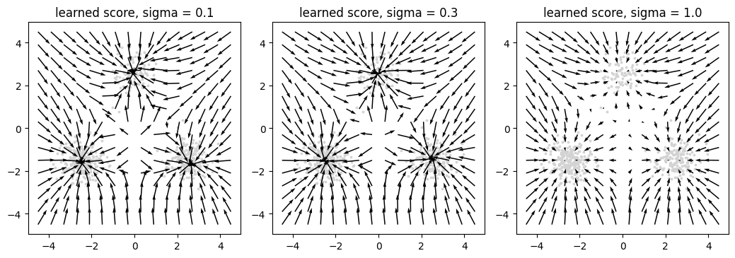

JAX

g = jnp.linspace(-4.5, 4.5, 16)
pts = jnp.stack(jnp.meshgrid(g, g, indexing='ij'), -1).reshape(-1, 2)
fig, axes = d2l.plt.subplots(1, 3, figsize=(10.5, 3.6))
for ax, (sigma, score) in zip(axes, scores.items()):
    f = score(pts)
    f = f * jnp.minimum(2 / jnp.linalg.norm(f, axis=1, keepdims=True), 1)
    ax.scatter(data[:500, 0], data[:500, 1], s=3, c='lightgray')
    ax.quiver(pts[:, 0], pts[:, 1], f[:, 0], f[:, 1], angles='xy',
              scale_units='xy', scale=2.5, width=0.005)
    ax.set_title(f'learned score, sigma = {sigma}'), ax.set_aspect('equal')
fig.tight_layout()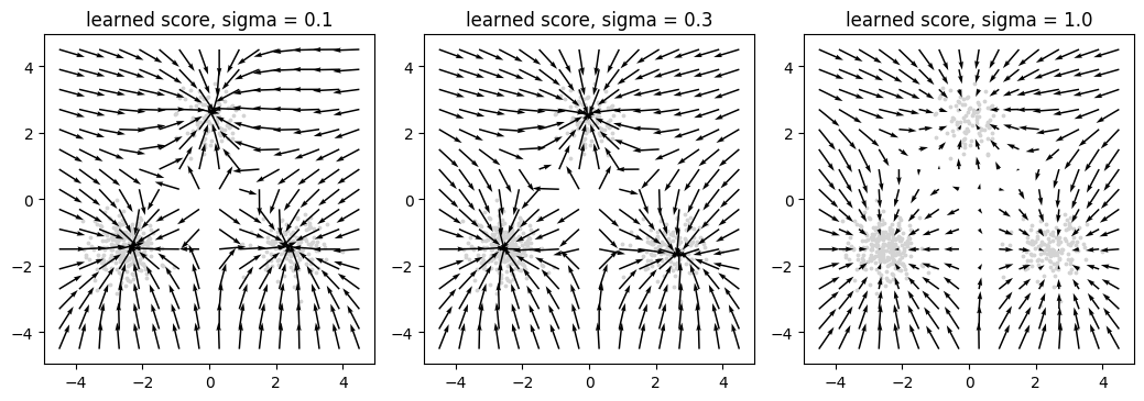

At the smallest noise level the field resembles the exact-score-matching result of Section 17.3: accurate near the modes, arbitrary in the empty regions. At the largest, the arrows are organized everywhere, including in the corners of the plot and in the region between the modes, because the noisy training points reached those places, but the field belongs to a smoother distribution. No single \(\sigma\) gives both properties. Section 17.6 resolves the tension by learning the score at every noise level of a ladder and using each where it is reliable.

17.4.4 Denoising Images

The denoising objective involves nothing that depends on the dimension of the input, so it applies unchanged to images. We use Fashion-MNIST (Section 3.2), with pixel values rescaled to \([-1, 1]\); on that scale a noise level of \(\sigma = 0.5\) corrupts the images heavily but not beyond recognition. The score network is a small convolutional network with one output channel, in the noise-prediction parameterization: it predicts \(\boldsymbol{\epsilon}\), and the score is its output divided by \(-\sigma\). The loss the cell minimizes is \(\sigma^2\) times the denoising objective averaged over pixels, which in the noise-prediction parameterization of Equation 17.4.2 is half the mean squared error of the noise prediction per pixel; the factor \(\sigma^2\) only rescales the objective and leaves its minimizer unchanged. Six hundred minibatch updates take about a minute on a laptop processor. The training data are loaded as a single tensor so that minibatches can be indexed directly.

PyTorch

fmnist = d2l.FashionMNIST(batch_size=128)
X = fmnist.train.data.float()[:, None] / 255 * 2 - 1  # (60000, 1, 28, 28)
X_test = fmnist.val.data.float()[:, None] / 255 * 2 - 1

class ConvDenoiser(nn.Module):
    def __init__(self, ch=32):
        super().__init__()
        self.net = nn.Sequential(nn.Conv2d(1, ch, 3, padding=1), nn.SiLU(),
                                 nn.Conv2d(ch, ch, 3, padding=1), nn.SiLU(),
                                 nn.Conv2d(ch, ch, 3, padding=1), nn.SiLU(),
                                 nn.Conv2d(ch, 1, 3, padding=1))

    def forward(self, x):  # predicts the noise; the score is -output / sigma
        return self.net(x)

sigma = 0.5
torch.manual_seed(0)
denoiser = ConvDenoiser()
image_score = lambda x: -denoiser(x) / sigma
optimizer = torch.optim.Adam(denoiser.parameters(), lr=1e-3)
for step in range(600):
    x = X[torch.randint(0, len(X), (128,))]
    eps = torch.randn_like(x)
    # sigma^2 times the per-pixel denoising objective: 0.5 E||eps_theta - eps||^2 / 784
    loss = 0.5 * sigma ** 2 * ((image_score(x + sigma * eps) + eps / sigma) ** 2).mean()
    optimizer.zero_grad(), loss.backward(), optimizer.step()
print(f'final training loss: {loss.item():.3f}')

final training loss: 0.061

JAX

fmnist = d2l.FashionMNIST(batch_size=128)
X = jnp.asarray(fmnist.train[0], jnp.float32)[..., None] / 255 * 2 - 1  # (60000, 28, 28, 1)
X_test = jnp.asarray(fmnist.val[0], jnp.float32)[..., None] / 255 * 2 - 1

class ConvDenoiser(nnx.Module):
    def __init__(self, ch=32, rngs=None):
        self.c1 = nnx.Conv(1, ch, (3, 3), padding='SAME', rngs=rngs)
        self.c2 = nnx.Conv(ch, ch, (3, 3), padding='SAME', rngs=rngs)
        self.c3 = nnx.Conv(ch, ch, (3, 3), padding='SAME', rngs=rngs)
        self.c4 = nnx.Conv(ch, 1, (3, 3), padding='SAME', rngs=rngs)

    def __call__(self, x):  # predicts the noise; the score is -output / sigma
        h = nnx.silu(self.c3(nnx.silu(self.c2(nnx.silu(self.c1(x))))))
        return self.c4(h)

sigma = 0.5
denoiser = ConvDenoiser(rngs=nnx.Rngs(0))
image_score = lambda x: -denoiser(x) / sigma
optimizer = nnx.Optimizer(denoiser, optax.adam(1e-3), wrt=nnx.Param)

@nnx.jit
def image_step(denoiser, optimizer, x, eps):
    def loss_fn(model):  # sigma^2 times the denoising objective
        s = -model(x + sigma * eps) / sigma
        return 0.5 * sigma ** 2 * ((s + eps / sigma) ** 2).mean()
    loss, grads = nnx.value_and_grad(loss_fn)(denoiser)
    optimizer.update(denoiser, grads)
    return loss

for step in range(600):
    key, k1, k2 = jax.random.split(key, 3)
    x = X[jax.random.randint(k1, (128,), 0, len(X))]
    loss = image_step(denoiser, optimizer, x, jax.random.normal(k2, x.shape))
print(f'final training loss: {loss:.3f}')

final training loss: 0.060

The final training loss, half the per-pixel squared error of the noise prediction on the last minibatch, is far below the value \(\tfrac12\) that predicting no noise at all would give, and it anticipates the denoising error measured next: the denoised image below differs from the clean one by \(\sigma (\boldsymbol{\epsilon} - \boldsymbol{\epsilon}_{\boldsymbol{\theta}})\), so its expected per-pixel squared error is \(2 \sigma^2 = 0.5\) times the expected loss, and the last minibatch’s loss of about \(0.06\) gives a rough estimate of \(0.03\). Tweedie’s formula Equation 17.4.4 converts the learned score into a denoiser: add \(\sigma^2\) times the score to the noisy image, which in the noise-prediction parameterization means subtracting \(\sigma\) times the predicted noise. The cell applies it to a thousand test images and compares the per-pixel squared error of the noisy input, which is \(\sigma^2 = 0.25\) in expectation, with that of the denoised output. The rows of the figure show clean, noisy, and denoised versions of the first eight test images.

PyTorch

with torch.no_grad():
    torch.manual_seed(1)
    x = X_test[:1000]
    x_noisy = x + sigma * torch.randn_like(x)
    x_denoised = x_noisy + sigma ** 2 * image_score(x_noisy)  # Tweedie
print(f'per-pixel squared error: noisy {((x_noisy - x) ** 2).mean():.3f}, '
      f'denoised {((x_denoised - x) ** 2).mean():.3f}')
imgs = torch.cat([x[:8], x_noisy[:8], x_denoised[:8]]).clamp(-1, 1) / 2 + 0.5
d2l.show_images(imgs.permute(0, 2, 3, 1).repeat(1, 1, 1, 3), 3, 8, scale=1.0);

per-pixel squared error: noisy 0.251, denoised 0.031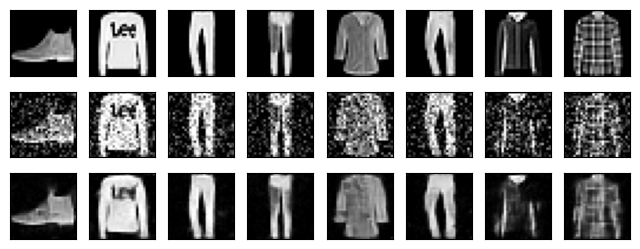

JAX

key, subkey = jax.random.split(key)
x = X_test[:1000]
x_noisy = x + sigma * jax.random.normal(subkey, x.shape)
x_denoised = x_noisy + sigma ** 2 * image_score(x_noisy)  # Tweedie
print(f'per-pixel squared error: noisy {((x_noisy - x) ** 2).mean():.3f}, '
      f'denoised {((x_denoised - x) ** 2).mean():.3f}')
imgs = jnp.concatenate([x[:8], x_noisy[:8], x_denoised[:8]]).clip(-1, 1) / 2 + 0.5
d2l.show_images(jnp.repeat(imgs, 3, -1), 3, 8, scale=1.0);

per-pixel squared error: noisy 0.250, denoised 0.031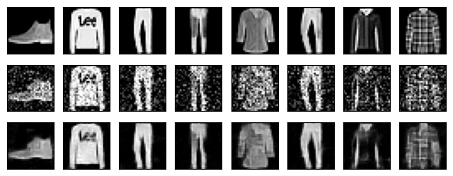

The network was trained to predict the noise, and the formula turned that prediction into a reconstruction whose error is a small fraction of the noise variance; given the noisy input, predicting the noise and predicting the clean image are the same task. The denoised images are smooth. A posterior mean averages over all clean images that could have produced the noisy one, so fine texture that the noise has destroyed is replaced by its average, an effect that grows with \(\sigma\). The samplers of later sections avoid it by drawing samples instead of averages: they remove the noise gradually and inject fresh noise at every step, or, like the deterministic samplers of Section 17.9 and Section 17.10, follow in small steps a flow that carries the noise distribution to the data distribution.

The model just trained is a score of Fashion-MNIST images at noise level \(0.5\), in \(784\) dimensions, fitted quickly with a regression loss. No partition function, no Markov chain, and no Jacobian were needed. What it does not provide is a sample. The next section builds the sampler.

17.4.5 Summary

Perturbing the data with Gaussian noise of scale \(\sigma\) gives a distribution \(p_\sigma\) whose density is positive and smooth everywhere. Its score can be learned by regression onto the conditional score \((\mathbf{x} - \tilde{\mathbf{x}}) / \sigma^2 = -\boldsymbol{\epsilon} / \sigma\), because the conditional mean of that target given the noisy point is \(\nabla \log p_\sigma(\tilde{\mathbf{x}})\); this is Vincent’s theorem, and it makes denoising score matching equivalent to score matching on \(p_\sigma\) without any Jacobian. Tweedie’s formula identifies the optimal model with the minimum-mean-squared-error denoiser, and the noise-prediction parameterization gives the regression a unit-variance target.

The noise level trades bias against variance. On the running example, a larger \(\sigma\) improved the fit to the perturbed score by more than an order of magnitude and covered the regions between the modes, while moving the learned field away from the score of the clean data. On Fashion-MNIST, a small convolutional network trained for six hundred updates learned the score at \(\sigma = 0.5\) well enough to reduce the per-pixel squared error of noisy images to a small fraction of the noise variance. The remaining questions are how to draw samples from a learned score and how to combine noise levels so that neither side of the trade-off is lost.

17.4.6 Exercises

1. Gaussian smoothing. Show that if \(p\) is a Gaussian with covariance \(\Sigma\), then \(p_\sigma\) is Gaussian with covariance \(\Sigma + \sigma^2 I\), and write both scores explicitly. For a one-dimensional standard Gaussian, compute the Fisher divergence between the clean and the perturbed score under the clean distribution as a function of \(\sigma\), and compare its value at \(\sigma = 0.3\) and \(\sigma = 1\) with the trend in the second column of the table.
2. The regression identity. Prove that for square-integrable \(Y\) and any function \(\mathbf{v}\), \(\mathbb{E}\|\mathbf{v}(X) - Y\|^2 = \mathbb{E}\|\mathbf{v}(X) - \mathbb{E}[Y \mid X]\|^2 + \mathbb{E}\|Y - \mathbb{E}[Y \mid X]\|^2\), by inserting and removing \(\mathbb{E}[Y \mid X]\) and conditioning on \(X\). Then explain why the denoising objective cannot reach zero for any data distribution that is not a single point, and, for the two-point data distribution \(p = \tfrac12 \delta_{-1} + \tfrac12 \delta_{+1}\) in one dimension at noise level \(\sigma\), write its minimum value as a one-dimensional integral and evaluate it numerically.
3. Tweedie’s formula. Derive Equation 17.4.4 from
   1. Then verify it in closed form for the two-point distribution of the previous exercise: compute the posterior mean \(\mathbb{E}[x \mid \tilde{x}]\) directly by Bayes’ rule and show that it equals \(\tilde{x} + \sigma^2 \frac{d}{d\tilde{x}} \log p_\sigma(\tilde{x})\). What does the denoiser return for \(\tilde{x} = 0\), and why is this the correct answer for the squared-error loss even though it is not a possible clean value?
4. [code] Estimated versus exact Bayes risk. For the running example the score of \(p_\sigma\) is known, so the minimum of the denoising objective can be estimated by evaluating Equation 17.4.2 with the true score of \(p_\sigma\) in place of the model. Compute this value for \(\sigma \in \{0.1, 0.3, 1.0\}\) on a large sample and compare it with the final training loss of each trained network. How much of each training loss is irreducible?
5. [code] Denoising at other noise levels. Apply the image denoiser trained at \(\sigma = 0.5\) to test images corrupted at \(\sigma = 0.25\) and \(\sigma = 1.0\), using Tweedie’s formula with the training noise level in both cases. Report the per-pixel squared error and describe the failure in each direction. What would be needed to handle several noise levels with a single network?
6. [code] A denoiser as a score. Train a convolutional network on Fashion-MNIST to predict the clean image directly from the noisy one with a squared-error loss, and convert its output into a score with \(\mathbf{s}(\tilde{\mathbf{x}}) = (D(\tilde{\mathbf{x}}) - \tilde{\mathbf{x}}) / \sigma^2\). Compare this score with the one learned by noise prediction on the same noisy test images by the mean squared difference between the two fields. Which parameterization is better conditioned as \(\sigma \to 0\), and why?

Bengio, Yoshua, Aaron Courville, and Pascal Vincent. 2013. “Representation Learning: A Review and New Perspectives.” IEEE Transactions on Pattern Analysis and Machine Intelligence 35 (8): 1798–828.

Efron, Bradley. 2011. “Tweedie’s Formula and Selection Bias.” Journal of the American Statistical Association 106 (496): 1602–14.

Kuleshov, Volodymyr. 2023. Deep Generative Models: Lecture Slides (Lectures 10–13: Advanced Topics in GANs, Energy-Based Models, Score-Based Generative Models, Diffusion Models). Course materials, Cornell Tech. Course website: https://kuleshov-group.github.io/dgm-website/; slides: https://github.com/kuleshov-group/dgm-resources.

Song, Yang, and Stefano Ermon. 2019. “Generative Modeling by Estimating Gradients of the Data Distribution.” Advances in Neural Information Processing Systems 32. https://arxiv.org/abs/1907.05600.

Vincent, Pascal. 2011. “A Connection Between Score Matching and Denoising Autoencoders.” Neural Computation 23 (7): 1661–74.