import numpy as np

rng = np.random.default_rng(0)
n = 1000
X_src = rng.normal(0.0, 1.0, (n, 2))            # source q: centered at (0, 0)
X_tgt = rng.normal(0.0, 1.0, (n, 2)) + [2, 0]   # target p: centered at (2, 0)
label = lambda X: (X[:, 1] > 0.5 * X[:, 0]**2 - 1).astype(float)
y_src, y_tgt = label(X_src), label(X_tgt)

def fit_logreg(X, y, weights=None, lr=0.1, steps=2000):
    w, b = np.zeros(X.shape[1]), 0.0
    v = np.ones(len(y)) if weights is None else weights / weights.mean()
    for _ in range(steps):
        g = v * (1 / (1 + np.exp(-(X @ w + b))) - y)   # weighted residual
        w -= lr * X.T @ g / len(y)
        b -= lr * g.mean()
return w, b3.7 Environment and Distribution Shift
The preceding analysis assumes that training and deployment data follow the same distribution. In practice, data collection, time, policy, and user behavior can change that distribution. A model with high test accuracy may then perform poorly after deployment. Deployment itself can also change the data distribution. Say, for example, that we trained a model to predict who will repay rather than default on a loan, finding that an applicant’s choice of footwear was associated with the risk of default (Oxfords indicate repayment, sneakers indicate default). We might be inclined thereafter to grant a loan to any applicant wearing Oxfords and to deny all applicants wearing sneakers.
This policy confuses a predictive association with a decision rule and ignores how applicants may respond. For starters, as soon as we began making decisions based on footwear, customers would catch on and change their behavior. Before long, all applicants would be wearing Oxfords, without any coincident improvement in credit-worthiness. Similar feedback occurs in many applications: model-based decisions can alter the environment that supplies later inputs. This is an instance of Goodhart’s law: when a measure becomes a target, it ceases to be a good measure.
This section identifies common forms of distribution shift, their assumptions, and several correction strategies. Some of the solutions are simple (ask for the “right” data), some are technically difficult (implement a reinforcement learning system), and others require policy and ethical analysis beyond statistical prediction.
3.7.1 Types of Distribution Shift
To begin, we stick with the passive prediction setting considering the various ways that data distributions might shift and what might be done to salvage model performance. In one classic setup, we assume that our training data was sampled from some distribution \(p_S(\mathbf{x},y)\) but that our test data will consist of unlabeled examples drawn from some different distribution \(p_T(\mathbf{x},y)\). Absent any assumptions on how \(p_S\) and \(p_T\) relate to each other, learning a classifier that works at test time is impossible.
Consider a binary classification problem, where we wish to distinguish between dogs and cats. If the distribution can shift in arbitrary ways, then our setup permits the pathological case in which the distribution over inputs remains constant: \(p_S(\mathbf{x}) = p_T(\mathbf{x})\), but the labels are all flipped: \(p_S(y \mid \mathbf{x}) = 1 - p_T(y \mid \mathbf{x})\). If the meanings of “cat” and “dog” swap without any change in the input distribution \(p(\mathbf{x})\), unlabeled target inputs cannot distinguish this case from one with no shift.
Under explicit restrictions on how the distribution changes, algorithms can sometimes detect the shift or adapt the classifier.
3.7.1.1 Covariate Shift
Among categories of distribution shift, covariate shift may be the most widely studied. Here, we assume that while the distribution of inputs may change over time, the labeling function, i.e., the conditional distribution \(P(y \mid \mathbf{x})\) does not change. Statisticians call this covariate shift because the problem arises due to a shift in the distribution of the covariates (features). While we can sometimes reason about distribution shift without invoking causality, we note that covariate shift is the natural assumption to invoke in settings where we believe that \(\mathbf{x}\) causes \(y\).
Consider the challenge of distinguishing cats and dogs. Our training data might consist of images of the kind in Figure 3.7.1.
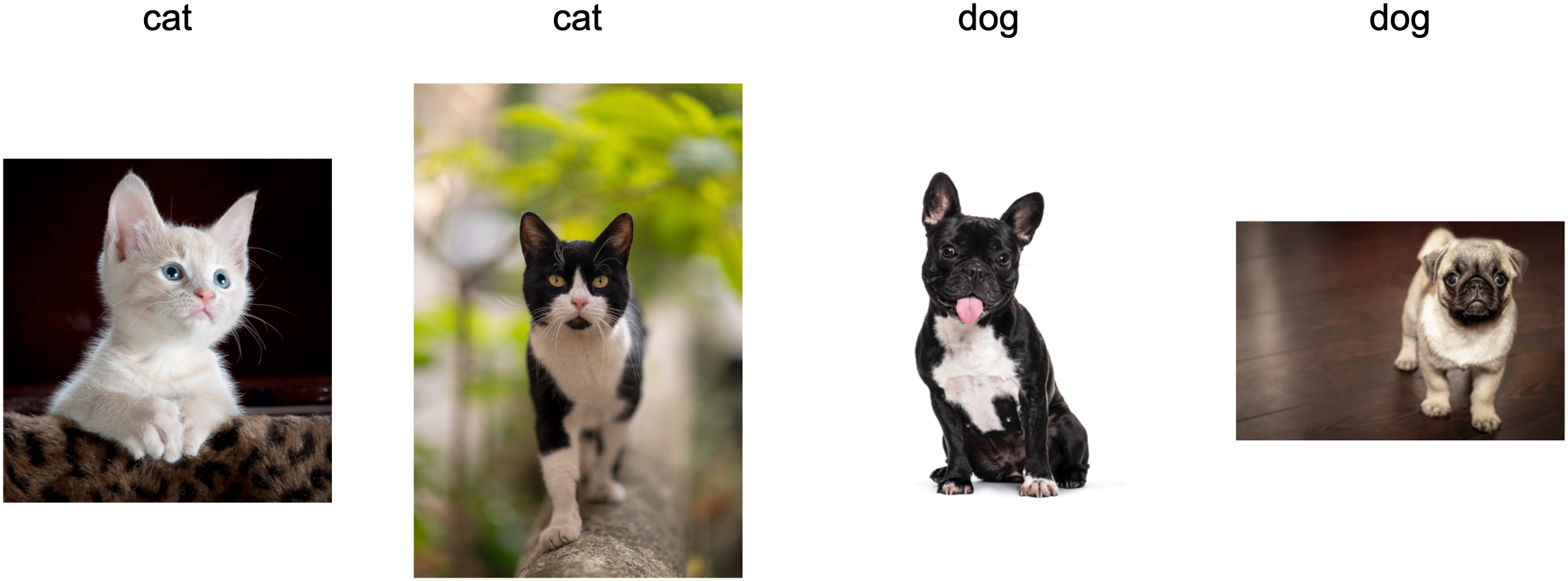
At test time we are asked to classify the images in Figure 3.7.2.

The training set consists of photos, while the test set contains only cartoons. Training on a dataset with substantially different characteristics from the test set can spell trouble absent a coherent plan for how to adapt to the new domain.
3.7.1.2 Label Shift
Label shift describes the converse problem. Here, we assume that the label marginal \(P(y)\) can change but the class-conditional distribution \(P(\mathbf{x} \mid y)\) remains fixed across domains. Label shift is a reasonable assumption to make when we believe that \(y\) causes \(\mathbf{x}\). For example, we may want to predict diagnoses given their symptoms (or other manifestations), even as the relative prevalence of diagnoses is changing over time. Label shift is the appropriate assumption here because diseases cause symptoms. In some degenerate cases the label shift and covariate shift assumptions can hold simultaneously. For example, when the label is deterministic, the covariate shift assumption will be satisfied, even when \(y\) causes \(\mathbf{x}\). Interestingly, in these cases, it is often advantageous to work with methods that flow from the label shift assumption. That is because these methods tend to involve manipulating objects that look like labels (often low-dimensional), as opposed to objects that look like inputs, which tend to be high-dimensional in deep learning.
3.7.1.3 Concept Shift
We may also encounter the related problem of concept shift, which arises when the very definitions of labels can change. This sounds weird (a cat is a cat, no?). However, other categories are subject to changes in usage over time. Diagnostic criteria for mental illness, what passes for fashionable, and job titles, are all subject to considerable amounts of concept shift. It turns out that if we navigate around the United States, shifting the source of our data by geography, we will find considerable concept shift regarding the distribution of names for soft drinks as shown in Figure 3.7.3.
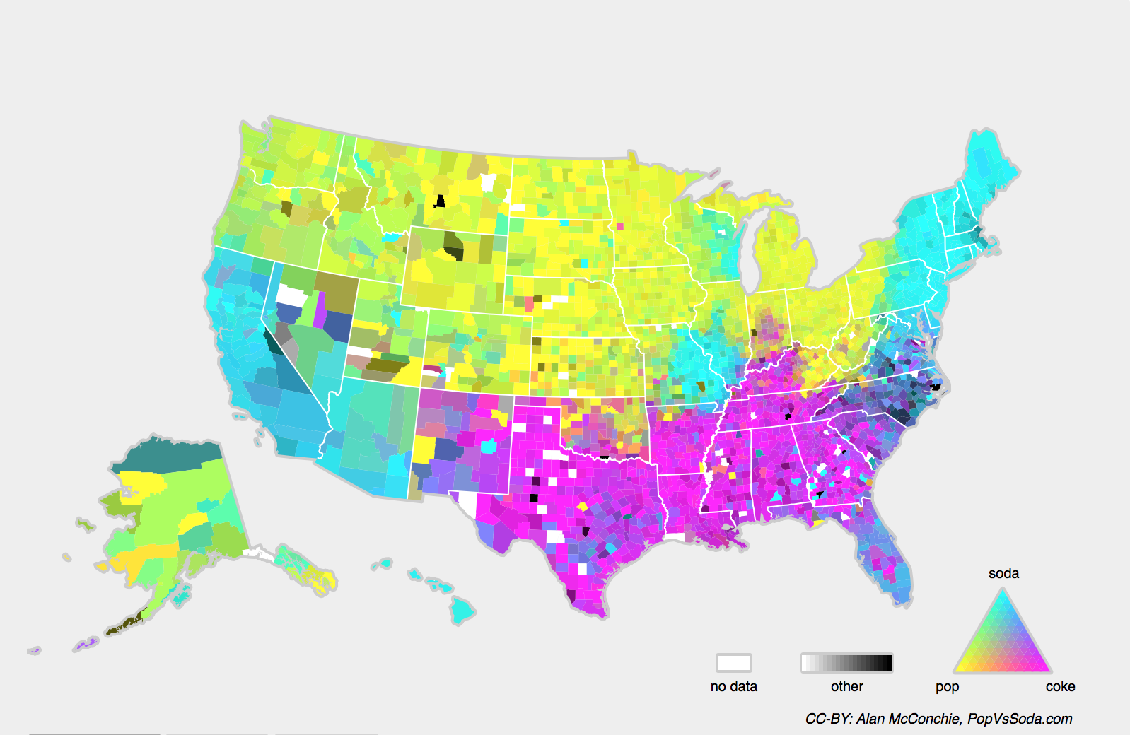
If we were to build a machine translation system, the distribution \(P(y \mid \mathbf{x})\) might be different depending on our location. This problem can be tricky to spot. We might hope to exploit knowledge that shift only takes place gradually either in a temporal or geographic sense.
3.7.2 Examples of Distribution Shift
Before turning to formalism and algorithms, we can discuss some concrete situations where covariate or concept shift might not be obvious.
3.7.2.1 Medical Diagnostics
Imagine that you want to design an algorithm to detect cancer. You collect data from healthy and sick people and you train your algorithm. It works fine, giving you high accuracy and you conclude that you are ready for a successful career in medical diagnostics. Not so fast.
The distributions that gave rise to the training data and those you will encounter in the wild might differ considerably. This happened to an unfortunate startup that some of us authors worked with years ago. They were developing a blood test for a disease that predominantly affects older men and hoped to study it using blood samples that they had collected from patients. However, it is considerably more difficult to obtain blood samples from healthy men than from sick patients already in the system. To compensate, the startup solicited blood donations from students on a university campus to serve as healthy controls in developing their test. Then they asked whether we could help them to build a classifier for detecting the disease.
As we explained to them, it would indeed be easy to distinguish between the healthy and sick cohorts with near-perfect accuracy. However, that is because the test subjects differed in age, hormone levels, physical activity, diet, alcohol consumption, and many more factors unrelated to the disease. This was unlikely to be the case with real patients. Due to their sampling procedure, we could expect to encounter extreme covariate shift. Moreover, this case was unlikely to be correctable via conventional methods. In short, they wasted a significant sum of money.
3.7.2.2 Self-Driving Cars
Say a company wanted to use machine learning for developing self-driving cars. One key component here is a roadside detector. Since real annotated data is expensive to get, they used synthetic data from a game-rendering engine as additional training data. Performance was high on held-out rendered data but poor on real images. As it turned out, the roadside had been rendered with a very simplistic texture. More importantly, all the roadside had been rendered with the same texture and the roadside detector learned about this “feature” very quickly.
A frequently repeated but poorly documented anecdote describes an attempt to train a neural network to detect tanks hidden among trees. They photographed a forest with no tanks, then drove tanks in and photographed it again, and the classifier reportedly performed well on held-out images but failed in the field. It had supposedly learned not to find tanks but to tell the tank-free photos from the rest: the two image sets differed in lighting and shadow (one set was taken in the early morning, the other at noon), not in their tanks. The anecdote is not reliable evidence, but it illustrates a genuine failure mode. A model can rely on a spurious feature when the training data do not vary that feature independently of the label; it need only correlate with the label in your sample and be absent in deployment.
3.7.2.3 Nonstationary Distributions
A nonstationary distribution arises when the distribution changes slowly (also known as nonstationary distribution) and the model is not updated adequately. Below are some typical cases.
- We train a computational advertising model and then fail to update it frequently (e.g., we forget to incorporate that an obscure new device called an iPad was just launched).
- We build a spam filter. It works well at detecting all spam that we have seen so far. Spammers then adapt and craft new messages that look unlike anything we have seen before.
- We build a product recommendation system. It works throughout the winter but then continues to recommend Santa hats long after Christmas.
3.7.2.4 Further Failure Modes
- We build a face detector. It works well on all benchmarks. It fails on test data when the offending examples are close-ups where the face fills the entire image (no such data was in the training set).
- We build a web search engine for the US market and want to deploy it in the UK.
- We train an image classifier by compiling a large dataset where each among a large set of classes is equally represented in the dataset, say 1000 categories, represented by 1000 images each. Then we deploy the system in the real world, where the actual label distribution of photographs is decidedly non-uniform.
3.7.3 Correction of Distribution Shift
As we have discussed, there are many cases where training and test distributions \(P(\mathbf{x}, y)\) are different. Some models continue to work despite covariate, label, or concept shift. In other cases, we can do better by employing principled strategies to cope with the shift. The remainder of this section develops two correction methods. It may be read independently of the later chapters, but its assumptions delimit exactly when unlabeled target data can support reweighting.
Recall from Section 2.6.1 the distinction between the empirical risk Equation 2.6.1 (the average loss on the training data) and the risk Equation 2.6.2 (the expected loss under the true data distribution \(p(\mathbf{x}, y)\)). In practice we cannot evaluate the risk directly and so we turn to empirical risk minimization, hoping that minimizing the empirical risk on the training set will approximately minimize the risk.
3.7.3.1 Covariate Shift Correction
Assume that we want to estimate some dependency \(P(y \mid \mathbf{x})\) for which we have labeled data \((\mathbf{x}_i, y_i)\). The observations \(\mathbf{x}_i\) are drawn from some source distribution \(q(\mathbf{x})\) rather than the target distribution \(p(\mathbf{x})\). The covariate-shift assumption means that the conditional distribution does not change: \(p(y \mid \mathbf{x}) = q(y \mid \mathbf{x})\). Although labeled observations come from \(q(\mathbf{x})\), we can express target risk as a reweighted source risk through the identity (Shimodaira 2000):
\[ \begin{aligned} \int\int l(f(\mathbf{x}), y) p(y \mid \mathbf{x})p(\mathbf{x}) \;d\mathbf{x}dy = \int\int l(f(\mathbf{x}), y) q(y \mid \mathbf{x})q(\mathbf{x})\frac{p(\mathbf{x})}{q(\mathbf{x})} \;d\mathbf{x}dy. \end{aligned} \tag{3.7.1}\]
In other words, we need to reweigh each data example by the ratio of the probability that it would have been drawn from the target distribution to that from the source distribution:
\[\beta_i \stackrel{\textrm{def}}{=} \frac{p(\mathbf{x}_i)}{q(\mathbf{x}_i)}.\]
Plugging in the weight \(\beta_i\) for each data example \((\mathbf{x}_i, y_i)\) we can train our model using weighted empirical risk minimization:
\[\mathop{\mathrm{minimize}}_f \frac{1}{n} \sum_{i=1}^n \beta_i l(f(\mathbf{x}_i), y_i). \tag{3.7.2}\]
Alas, we do not know that ratio, so before we can do anything useful we need to estimate it. Many methods estimate this ratio directly, matching moments of the reweighted source to the target without ever estimating \(p\) and \(q\) separately (Gretton et al. 2012). Note that for any such approach, we need samples drawn from both distributions: the “true” \(p\), e.g., by access to test data, and the one used for generating the training set \(q\) (the latter is trivially available). Note however, that we only need features \(\mathbf{x} \sim p(\mathbf{x})\); we do not need to access labels \(y \sim p(y)\).
In this case, there exists a very effective approach that will give almost as good results as the original: namely, logistic regression, which is a special case of softmax regression (see Section 3.1) for binary classification. This is all that is needed to compute estimated probability ratios. We learn a classifier to distinguish between data drawn from \(p(\mathbf{x})\) and data drawn from \(q(\mathbf{x})\). If it is impossible to distinguish between the two distributions then it means that the associated instances are equally likely to come from either one of those two distributions. On the other hand, any instances that can be well discriminated should be significantly overweighted or underweighted accordingly.
For simplicity’s sake assume that we have an equal number of instances from both distributions \(p(\mathbf{x})\) and \(q(\mathbf{x})\), respectively. Now denote by \(z\) labels that are \(1\) for data drawn from \(p\) and \(-1\) for data drawn from \(q\). Then the probability in a mixed dataset is given by
\[P(z=1 \mid \mathbf{x}) = \frac{p(\mathbf{x})}{p(\mathbf{x})+q(\mathbf{x})} \textrm{ and hence } \frac{P(z=1 \mid \mathbf{x})}{P(z=-1 \mid \mathbf{x})} = \frac{p(\mathbf{x})}{q(\mathbf{x})}.\]
Thus, if we use a logistic regression approach, where \(P(z=1 \mid \mathbf{x})=\frac{1}{1+\exp(-h(\mathbf{x}))}\) (\(h\) is a parametrized function), it follows that
\[ \beta_i = \frac{1/(1 + \exp(-h(\mathbf{x}_i)))}{\exp(-h(\mathbf{x}_i))/(1 + \exp(-h(\mathbf{x}_i)))} = \exp(h(\mathbf{x}_i)). \]
(With unequal sample sizes \(\exp(h)\) estimates \(p/q\) only up to the constant \(m/n\), which does not affect the weighted minimizer.)
As a result, we need to solve two problems: first distinguish source from target data, and then a weighted empirical risk minimization problem in Equation 3.7.2 where we weigh terms by \(\beta_i\).
Now we are ready to describe a correction algorithm. Suppose that we have a training set \(\{(\mathbf{x}_1, y_1), \ldots, (\mathbf{x}_n, y_n)\}\) and an unlabeled test set \(\{\mathbf{u}_1, \ldots, \mathbf{u}_m\}\). For covariate shift, we assume that \(\mathbf{x}_i\) for all \(1 \leq i \leq n\) are drawn from some source distribution and \(\mathbf{u}_i\) for all \(1 \leq i \leq m\) are drawn from the target distribution. Here is a prototypical algorithm for correcting covariate shift:
- Create a binary-classification training set from source and target features. Balance the two domain classes by subsampling or class weighting; otherwise include the known domain-prior correction in the odds.
- Train a binary classifier using logistic regression to get the function \(h\).
- Weigh training data using \(\beta_i = \exp(h(\mathbf{x}_i))\) or better \(\beta_i = \min(\exp(h(\mathbf{x}_i)), c)\) for some constant \(c\).
- Use weights \(\beta_i\) for training on \(\{(\mathbf{x}_1, y_1), \ldots, (\mathbf{x}_n, y_n)\}\) in Equation 3.7.2.
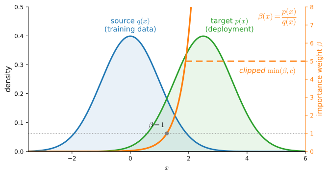
Clipping the weights at a ceiling \(c\) trades a little bias for much lower variance: when source and target barely overlap, a handful of examples acquire enormous weights \(\beta_i\) that would otherwise dominate and destabilize the weighted objective. Figure 3.7.4 shows the geometry of the whole construction: where the target density \(p\) exceeds the source density \(q\), the ratio \(\beta = p/q\) grows, and it grows exponentially fast out in the tail where the source has almost no mass, which is exactly where the clip takes over.
Note that the above algorithm relies on one assumption. For this scheme to work, we need that each data example in the target (e.g., test time) distribution had nonzero probability of occurring at training time. If we find a point where \(p(\mathbf{x}) > 0\) but \(q(\mathbf{x}) = 0\), then the corresponding importance weight should be infinity.
3.7.3.1.1 Covariate Shift Correction in Code
The following two-dimensional example implements the discriminator and reweighted training pipeline. We make the shift two-dimensional so that the shift is visible: source inputs are Gaussian around the origin, target inputs are the same Gaussian shifted to be centered at \((2, 0)\), and both share one labeling rule (covariate shift by construction). The label depends on \(\mathbf{x}\) through a curved boundary, so a linear classifier is misspecified and it matters where it spends its capacity. The only trainer we need is logistic regression by gradient descent, with an optional per-example weight:
Step one of the algorithm: pool the source inputs (labeled \(z=0\)) with the unlabeled target inputs (\(z=1\)) and train the domain discriminator \(h\). For two unit Gaussians the true log-density-ratio is exactly linear, \(\log (p(\mathbf{x})/q(\mathbf{x})) = 2x_1 - 2\), so we can check the learned \(h\) against the truth, and the weights are \(\beta_i = \exp(h(\mathbf{x}_i))\):
w_h, b_h = fit_logreg(np.concatenate([X_src, X_tgt]),
                      np.concatenate([np.zeros(n), np.ones(n)]))
beta = np.exp(X_src @ w_h + b_h)
print(f'learned h(x) = {w_h[0]:.2f} x1 {w_h[1]:+.2f} x2 {b_h:+.2f} '
      f'(true log-ratio: 2 x1 - 2)')
print(f'beta on source data: mean {beta.mean():.2f}, max {beta.max():.1f}')
learned h(x) = 2.06 x1 +0.09 x2 -2.03 (true log-ratio: 2 x1 - 2)
beta on source data: mean 0.86, max 56.2Step two: train the actual classifier three ways, on the same source data with the same labels, and evaluate each on the target domain, which is the one we care about:
acc = lambda wb, X, y: ((X @ wb[0] + wb[1] > 0) == (y > 0.5)).mean()
for name, wts in [('unweighted', None), ('weighted', beta),
                  ('clipped, c=5', np.minimum(beta, 5))]:
    wb = fit_logreg(X_src, y_src, wts)
    print(f'{name:12s}  target accuracy: {acc(wb, X_tgt, y_tgt):.3f}'
          f'   (source accuracy: {acc(wb, X_src, y_src):.3f})')
unweighted target accuracy: 0.502 (source accuracy: 0.860)
weighted target accuracy: 0.933 (source accuracy: 0.795)
clipped, c=5 target accuracy: 0.945 (source accuracy: 0.817)In this seeded construction, the unweighted model fits the source region and performs near chance on the target domain. Reweighting raises target accuracy above 90% at the cost of a worse source fit, as Equation 3.7.1 predicts. The largest raw weight exceeds 50, so clipping at \(c=5\) reduces the influence of a few source points and happens to improve this run slightly. Repeated seeds or confidence intervals are needed before treating that last comparison as systematic. Exercises 3 and 4 probe when this pipeline fails as the target moves away from the source, although the supports of the two Gaussians always overlap.
3.7.3.2 Label Shift Correction
Assume that we are dealing with a classification task with \(k\) categories. Using the same notation in Section 3.7.3.1, \(q\) and \(p\) are the source distribution (e.g., training time) and target distribution (e.g., test time), respectively. Assume that the distribution of labels shifts over time: \(q(y) \neq p(y)\), but the class-conditional distribution stays the same: \(q(\mathbf{x} \mid y)=p(\mathbf{x} \mid y)\). If the source distribution \(q(y)\) is “wrong”, we can correct for that according to the following identity in the risk as defined in Equation 2.6.2:
\[ \begin{aligned} \int\int l(f(\mathbf{x}), y) p(\mathbf{x} \mid y)p(y) \;d\mathbf{x}dy = \int\int l(f(\mathbf{x}), y) q(\mathbf{x} \mid y)q(y)\frac{p(y)}{q(y)} \;d\mathbf{x}dy. \end{aligned} \]
Here, our importance weights will correspond to the label likelihood ratios:
\[\beta_i \stackrel{\textrm{def}}{=} \frac{p(y_i)}{q(y_i)}. \tag{3.7.3}\]
One nice thing about label shift is that if we have a reasonably good model on the source distribution, then we can get consistent estimates of these weights without ever having to deal with the ambient dimension. In deep learning, the inputs tend to be high-dimensional objects like images, while the labels are often simpler objects like categories.
To estimate the target label distribution, we first take our reasonably good off-the-shelf classifier (typically trained on the training data) and compute its confusion matrix \(\mathbf{C}\) on the validation set (also from the training distribution). Recall the \(k \times k\) confusion matrix of Section 3.3, column-normalized exactly as we computed it in Section 3.4: entry \(c_{ij}\) is the fraction of validation examples of true class \(j\) that the model predicted as class \(i\), so each column sums to \(1\) and estimates \(P(\hat{y}=i \mid y=j)\).
Now, we cannot calculate the confusion matrix on the target data directly because we do not get to see the labels for the examples that we see in the wild, unless we invest in a complex real-time annotation pipeline. What we can do, however, is average all of our model’s predictions at test time together, yielding the mean model outputs \(\mu(\hat{\mathbf{y}}) \in \mathbb{R}^k\), where the \(i^\textrm{th}\) element \(\mu(\hat{y}_i)\) is the fraction of the total predictions on the test set where our model predicted \(i\).
It turns out that under some mild conditions, namely that our classifier was reasonably accurate in the first place, that the target data contains only categories that we have seen before, and that the label shift assumption holds in the first place (the strongest assumption here), we can estimate the test set label distribution by solving a simple linear system
\[\mathbf{C} p(\mathbf{y}) = \mu(\hat{\mathbf{y}}), \tag{3.7.4}\]
because as an estimate \(\sum_{j=1}^k c_{ij} p(y_j) = \mu(\hat{y}_i)\) holds for all \(1 \leq i \leq k\), where \(p(y_j)\) is the \(j^\textrm{th}\) element of the \(k\)-dimensional label distribution vector \(p(\mathbf{y})\). If our classifier is accurate enough that \(\mathbf{C}\) is diagonally dominant (each class is predicted correctly more often than it is mistaken for any collection of others), then \(\mathbf{C}\) will be invertible, and we get a solution \(p(\mathbf{y}) = \mathbf{C}^{-1} \mu(\hat{\mathbf{y}})\). This confusion-matrix estimator goes back to Saerens et al. (2002); Lipton et al. (2018) showed that, treating the trained classifier as a black box, it yields consistent estimates of the target label distribution under the label-shift assumption (an approach they call black-box shift estimation).
Because we observe the labels on the source data, it is easy to estimate the distribution \(q(y)\). Then, for any training example \(i\) with label \(y_i\), we can take the ratio of our estimated \(p(y_i)/q(y_i)\) to calculate the weight \(\beta_i\), and plug this into weighted empirical risk minimization in Equation 3.7.2.
3.7.3.3 Concept Shift Correction
Concept shift requires information about the changed labeling relation. For instance, in a situation where suddenly the problem changes from distinguishing cats from dogs to one of distinguishing white from black animals, new labeled data may be necessary, potentially followed by retraining. Some concept shifts are gradual rather than abrupt. To make things more concrete, here are some examples:
- In computational advertising, new products are launched, old products become less popular. This means that the distribution over ads and their popularity changes gradually and any click-through rate predictor needs to change gradually with it.
- Traffic camera lenses degrade gradually due to environmental wear, affecting image quality progressively.
- News content changes gradually (i.e., most of the news remains unchanged but new stories appear).
For gradual shift, one possible response is to retain the current weights and perform update steps on fresh labeled data. Its suitability depends on the rate and form of the shift.
3.7.4 Beyond Static Supervised Learning
This chapter studies supervised prediction under distribution shift. Other problem formulations change the information available to the learner: online learning reveals observations sequentially, bandits reveal rewards only for chosen actions, and reinforcement learning allows actions to alter later states. Those settings require their own notation and algorithms and are developed in the corresponding later chapters. Here the relevant boundary is simpler: once deployment decisions change future data, the evaluation distribution is partly produced by the model itself.
3.7.5 Deployment Decisions and Feedback
Deploying a model often turns predictions into decisions that affect both people and the data observed later. A medical classifier, for example, must be evaluated across relevant populations and against the costs of different errors, not only by aggregate accuracy. Thresholds should therefore be chosen from an explicit loss model and evaluated separately for affected groups. Threshold adjustment alone does not establish fairness: different fairness criteria can conflict, and the labels, data-collection process, and decision policy may themselves create harm. This section identifies the connection to distribution shift; a dedicated treatment is needed for competing fairness definitions and their limitations.
Decisions can also create feedback loops. Consider predictive policing systems, which allocate patrol officers to areas with high forecasted crime. It is easy to see how a worrying pattern can emerge:
- Neighborhoods with more crime get more patrols.
- Consequently, more crimes are discovered in these neighborhoods, entering the training data available for future iterations.
- Exposed to more positives, the model predicts yet more crime in these neighborhoods.
- In the next iteration, the updated model targets the same neighborhood even more heavily leading to yet more crimes discovered, etc.
The model’s decisions change where labels are collected, which changes the next training distribution and reinforces the original allocation. Monitoring this coupling is part of distribution-shift analysis, but it does not replace a normative assessment of whether the decision system serves an appropriate goal.
3.7.6 Summary
In many cases training and test sets do not come from the same distribution. This is called distribution shift. The risk is the expectation of the loss over the entire population of data drawn from their true distribution. However, this entire population is usually unavailable. Empirical risk is an average loss over the training data to approximate the risk. In practice, we perform empirical risk minimization.
Under covariate- or label-shift assumptions, unlabeled target data can support specific reweighting corrections. A change in the input marginal may be detectable without labels, but the claim that \(P(y\mid\mathbf{x})\) or \(P(\mathbf{x}\mid y)\) stayed fixed is not generally identifiable from those data alone. Corrections therefore depend on an assumption that must be defended from domain knowledge and checked when target labels become available. Automated actions can affect later observations. Deployment monitoring should therefore track both predictive performance and feedback between the model and its environment.
These ideas predate the current era of large pretrained models, but distribution shift remains central because a foundation model is routinely deployed on domains, users, and time periods unlike its training corpus. Curated benchmarks such as WILDS (Koh et al. 2021) show that models with strong in-distribution accuracy can still degrade sharply out of distribution, and that a correction which helps on one shift often fails on another, so evaluation should represent the deployment shifts of interest.
3.7.7 Exercises
Feedback loops. A search engine changes how it ranks results. It then retrains its ranker on the clicks logged under the new ranking, with a query-document pair as the input \(\mathbf{x}\) and a click as the label \(y\).
- Describe one way users and one way advertisers might respond to the new ranking.
- For each response, state whether it changes \(p(\mathbf{x})\), \(p(y \mid \mathbf{x})\), or both in the next training set. Then decide whether the response is an instance of Goodhart’s law.
Covariate-shift identity. The covariate-shift assumption is \(p(y \mid \mathbf{x}) = q(y \mid \mathbf{x})\).
- Starting from the risk under the target distribution \(p(\mathbf{x}, y)\), derive Equation 3.7.1, whose sample version is the weighted objective Equation 3.7.2. Mark the step that uses the assumption and the step that requires \(q(\mathbf{x}) > 0\) wherever \(p(\mathbf{x}) > 0\).
- Suppose \(p(\mathbf{x}) > 0\) on a region where \(q(\mathbf{x}) = 0\). Which part of the target risk does the reweighted source risk omit, and why can no choice of weights on source examples recover it?
[code] When reweighting fails. The pipeline of Section 3.7.3.1 (
fit_logreg,X_src,X_tgt,label) places the target mean at \((2, 0)\). Sweep the target mean over \((s, 0)\) for \(s \in \{0, 0.5, 1, 2, 3, 4, 6\}\), keeping \(n = 1000\) and the labeling rule fixed.- For each \(s\), report the accuracy of the domain classifier \(h\) on held-out pooled data, and interpret its growth with \(s\) in terms of how detectable the shift is.
- For each \(s\), record the target accuracy of the unweighted, weighted, and clipped (\(c = 5\)) models, and of the constant predictor that outputs the majority class of
y_tgt. Explain why target accuracy alone cannot show whether reweighting worked at large \(s\).
[code] Learned versus true weights. ● Reuse the sweep of exercise 3 over target means \((s, 0)\).
- Derive the true log-ratio \(\log(p(\mathbf{x})/q(\mathbf{x}))\) as a function of \(s\), and compare it with the learned \(h\) at each \(s\). Explain how the domain classifier can reach high accuracy at large \(s\) while \(h\) is far from the true log-ratio.
- Both input distributions are Gaussian, so \(q(\mathbf{x}) > 0\) wherever \(p(\mathbf{x}) > 0\) for every \(s\). For each \(s\), compute the effective sample size \((\sum_i \beta_i)^2 / \sum_i \beta_i^2\) of the source data under the learned weights \(\beta_i = \exp(h(\mathbf{x}_i))\) and under the true weights \(p(\mathbf{x}_i)/q(\mathbf{x}_i)\). Explain why the true weights leave only a few effective source examples at large \(s\) although no weight is infinite. Relate the difference between the two effective sample sizes to the gap between \(h\) and the true log-ratio, and say whether clipping at \(c = 5\) repairs the shortage.
Label-shift linear system. A \(k\)-class classifier has the column-normalized validation confusion matrix \(\mathbf{C}\) with entries \(c_{ij} = q(\hat{y} = i \mid y = j)\), and its predictions on unlabeled target data have mean \(\mu(\hat{\mathbf{y}})\).
- Derive \(\mathbf{C}\, p(\mathbf{y}) = \mu(\hat{\mathbf{y}})\) from the law of total probability, and identify the step that uses the label-shift assumption \(q(\mathbf{x} \mid y) = p(\mathbf{x} \mid y)\).
- Give an example of a classifier for which \(\mathbf{C}\) is singular, and describe what \(\mu(\hat{\mathbf{y}})\) can still reveal about \(p(\mathbf{y})\) in that case.
- Both \(\mathbf{C}\) and \(\mu(\hat{\mathbf{y}})\) are estimated from finite samples. Explain how errors in \(\mu(\hat{\mathbf{y}})\) propagate to \(\mathbf{C}^{-1}\mu(\hat{\mathbf{y}})\) when \(\mathbf{C}\) is nearly singular.
Shift assumptions from unlabeled data. ● In a binary source domain, \(q(y = 1) = q(y = 0) = 1/2\), and the scalar input satisfies \(x \mid y = 1 \sim \mathcal{N}(1, 1)\) and \(x \mid y = 0 \sim \mathcal{N}(-1, 1)\). Hence \(q(y = 1 \mid x) = 1/(1 + \exp(-2x))\). Unlabeled target inputs follow the mixture
\[p(x) = 0.8\, \mathcal{N}(x; 1, 1) + 0.2\, \mathcal{N}(x; -1, 1). \tag{3.7.5}\]
- Assume label shift. Give \(p(y = 1)\) and the threshold on \(x\) of the Bayes-optimal target classifier.
- Assume instead covariate shift with the same \(p(x)\). Compute \(p(y = 1)\) numerically and give the Bayes-optimal threshold.
- Use your results to explain why no statistic of the unlabeled target sample can decide which of the two corrections of this section applies.
Features missing at serving time. A model forecasts a store’s daily revenue at the start of each day. Its training records hold each past day’s final customer count as a feature, and the model performs well in offline evaluation on held-out records. At serving time the pipeline fills this feature with the number of customers counted so far that day.
- Compare the distribution of this feature, and its relation to revenue, in the training records and at serving time. State which of the section’s shift assumptions, if any, holds between the two.
- Explain why the offline evaluation could not reveal this mismatch, and why the reweighting of Section 3.7.3.1 cannot repair it.
- Propose a rule for selecting training features that avoids this failure.
Adapted from Google’s Machine Learning Crash Course, “Monitoring pipelines”.
[extended] Real-world shifts. The WILDS benchmark (Koh et al. 2021) catalogs distribution shifts collected in the wild. Pick two of its tasks, for example a hospital-to-hospital or a camera-trap-to-camera-trap shift, and classify each as closer to covariate shift, label shift, or neither, justifying your classification from how the data were collected. If you can download one of the smaller WILDS datasets, train a linear baseline and report its in-distribution versus out-of-distribution accuracy gap.