%matplotlib inline
from d2l import torch as d2l
import numpy as np29.2 Stochastic Differential Equations
Diffusion models use a forward noising SDE to transform data toward a Gaussian reference distribution. This section develops three ingredients needed for DDPM (Ho et al. 2020) and score-based models (Song et al. 2021): Brownian motion, Itô calculus, and the Ornstein–Uhlenbeck process underlying variance-preserving diffusion. These tools give a precise and simulatable account of the forward process; Section 29.3 studies its reversal.
A Brownian increment over a time step \(\Delta t\) has scale \(\sqrt{\Delta t}\) rather than \(\Delta t\), so noise dominates drift over short intervals. Its square, \((\Delta W)^2 \approx \Delta t\), remains a first-order quantity. Consequently, the second-order Taylor term that ordinary calculus discards survives as a first-order effect. The Itô correction, the form of Itô’s lemma, the \(\sqrt{\Delta t}\) noise kick in the Euler–Maruyama scheme, and the convergence rates of that scheme all follow from this scaling.
We lean on Section 29.1 (vector fields, the forward Euler method, linear stability), and on Section 27.1 and Section 27.2 (Gaussians, expectation, variance, independence). Introductory and rigorous treatments are provided by Särkkä and Solin (2019) and Øksendal (2003), respectively; the numerical theory is Kloeden and Platen (1992) . The code in this section is plain NumPy: every experiment is a seeded simulation plus a closed-form check; the d2l module is loaded only for plotting.
%matplotlib inline
from d2l import tensorflow as d2l
import numpy as np%matplotlib inline
from d2l import jax as d2l
import numpy as np%matplotlib inline
from d2l import mxnet as d2l
import numpy as np29.2.1 Brownian Motion
29.2.1.1 Randomness as a Data-Independent Noising Mechanism
Section 29.1 gave us a deterministic law of motion: a velocity field \(\mathbf{f}\) moves every point along the one trajectory through it, and the resulting exact flow map is invertible under the well-posedness conditions of Section 29.1. This is useful for deterministic transport, whereas the forward process of a diffusion model must erase information in a controlled manner: starting from data distributed as \(p_0 = p_{\textrm{data}}\), it should end at a known, distribution-independent target,
\[ p_0 = p_{\textrm{data}} \;\longrightarrow\; p_T \approx \mathcal{N}(\mathbf{0}, \sigma^2 I), \]
so that at generation time we always know what to sample as a starting point, no matter what the data looked like. Deterministic flows cannot do this job universally. A fixed map sends point masses to point masses, never to a Gaussian; and the ODE flows of Section 29.1 are bijections, so distinct data laws stay distinct. (A learned, data-dependent deterministic flow does carry one given \(p_{\textrm{data}}\) to the Gaussian; that is exactly what flow matching will build in Section 29.4.3, but such a map must be discovered by training. The forward process must be defined independently of learned parameters and the particular data distribution.) Adding noise instead progressively reduces information about the data. The distribution at each intermediate time is a smoothed, full-dimensional version of the data, and the process can be run in reverse on average once we know the score of those blurred distributions, the gradient \(\nabla \log p_t\) of the log-density (Section 29.3). The object that accomplishes all this is a stochastic differential equation, an ordinary ODE with a noise term:
\[ d\mathbf{X} \;=\; \underbrace{\mathbf{f}(\mathbf{X}, t)\,dt}_{\textrm{drift}} \;+\; \underbrace{g(t)\,d\mathbf{W}}_{\textrm{diffusion}}. \tag{29.2.1}\]
The remainder of the section defines the noise source \(\mathbf{W}\), develops Itô calculus to give Equation 29.2.1 a precise meaning, introduces Euler–Maruyama simulation, and analyzes the Ornstein–Uhlenbeck process used by diffusion models.
29.2.1.2 From Random Walks to the Wiener Process
Brownian motion is what a simple random walk becomes when its steps shrink. Fix a step duration \(\Delta t\) and let a walker take independent steps of size \(\pm\sqrt{\Delta t}\), each sign chosen by a fair coin. After \(k\) steps, i.e. at time \(t = k\,\Delta t\), the position is a sum of \(k\) independent, mean-zero steps of variance \(\Delta t\) apiece, so variances add (Section 27.1) to give
\[ \mathbb{E}\!\left[W^{(\Delta t)}_t\right] = 0, \qquad \operatorname{Var}\!\left(W^{(\Delta t)}_t\right) = k\,\Delta t = t, \]
independently of the step size. The exponent in that step size is forced. Steps of size \(c\,\Delta t\) would give variance \(c^2 t\,\Delta t \to 0\), so the limiting process is constant. Steps of fixed size \(c\) would give variance \(c^2 t / \Delta t \to \infty\): the variance diverges. Only the square-root scaling \(\sqrt{\Delta t}\) produces a nontrivial limit; it returns as the noise term of every numerical scheme below. As \(\Delta t \to 0\) the number of steps before time \(t\) grows without bound, and the central limit theorem (a sum of many independent, mean-zero contributions with total variance \(t\) is approximately \(\mathcal{N}(0, t)\)) makes the limiting position Gaussian. The limit process is called Brownian motion or the Wiener process (Wiener 1923), and its defining properties are
- \(W_0 = 0\);
- independent increments: for \(s < t\), the increment \(W_t - W_s\) is independent of the entire path up to time \(s\);
- Gaussian increments: \(W_t - W_s \sim \mathcal{N}(0,\, t - s)\);
- continuous sample paths.
The central limit theorem above pins down only the one-time marginals; the hard content is that a process with properties 1–4 exists at all and is the limit of the rescaled walks. We take both facts as given: existence is Wiener’s theorem (Wiener 1923), and the convergence of the walks is Donsker’s invariance principle.
In particular \(\mathbb{E}[W_t] = 0\) and \(\operatorname{Var}(W_t) = t\): the process spreads, with standard deviation \(\sqrt{t}\), forever (Figure 29.2.1). Simulation uses the increment form
\[ \Delta W \;=\; W_{t + \Delta t} - W_t \;=\; \sqrt{\Delta t}\;\xi, \qquad \xi \sim \mathcal{N}(0, 1). \tag{29.2.2}\]
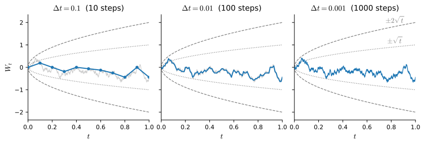
The multivariate version \(\mathbf{W}_t\) runs one independent scalar Brownian motion per coordinate; for the diagonal, state-independent noise \(g(t)\,d\mathbf{W}\) used throughout this chapter, the calculations below extend coordinate-wise. Two consequences of the definition are used below. The first is the correlation structure.
Proposition (covariance of Brownian motion). For all \(s, t \ge 0\), \(\operatorname{Cov}(W_s, W_t) = \min(s, t)\).
Proof. Take \(s \le t\) and split \(W_t = W_s + (W_t - W_s)\). Then
\[ \mathbb{E}[W_s W_t] = \mathbb{E}\!\left[W_s^2\right] + \mathbb{E}\!\left[W_s (W_t - W_s)\right] = s + \mathbb{E}[W_s]\,\mathbb{E}[W_t - W_s] = s, \]
where the cross term factorizes because the increment \(W_t - W_s\) is independent of \(W_s\), and both factors have mean zero. Since the means vanish, \(\operatorname{Cov}(W_s, W_t) = \mathbb{E}[W_s W_t] = \min(s, t)\). \(\blacksquare\)
The second consequence motivates stochastic integration. Brownian paths are almost surely continuous but nowhere differentiable, a theorem (Paley et al. 1933). The increment scaling supplies a useful heuristic: Equation 29.2.2:
\[ \left|\frac{\Delta W}{\Delta t}\right| = \frac{|\xi|}{\sqrt{\Delta t}} \;\longrightarrow\; \infty \quad \textrm{in probability as } \Delta t \to 0. \]
Thus a fresh difference quotient does not remain bounded in probability. This scaling is not a proof of the pathwise theorem: increments at nested scales are dependent, and nowhere differentiability requires a separate argument. It does explain the obstruction. A differentiable curve has a tangent under local rescaling (Section 25.1), whereas a Brownian path retains fluctuations at every scale with the same rescaled statistical structure. Thus “\(dW/dt\)” does not exist, and a velocity-field reading of Equation 29.2.1 is unavailable: we will have to make sense of \(dW\) inside integrals, which is exactly what the Itô calculus does.
29.2.1.3 Simulating Path Ensembles
The increment form Equation 29.2.2 is a simulation recipe: cumulatively sum \(\sqrt{\Delta t}\,\xi\) steps. We generate \(20{,}000\) paths on \([0, 1]\) and check the variance law \(\operatorname{Var}(W_t) = t\) at several times, plotting a few paths against the \(\pm 2\sqrt{t}\) envelope that should contain about \(95\%\) of them.
rng = np.random.default_rng(42)
T, n, n_paths = 1.0, 500, 20000
dt = T / n
t = np.linspace(0, T, n + 1)
dW = np.sqrt(dt) * rng.standard_normal((n_paths, n))
W = np.concatenate([np.zeros((n_paths, 1)), np.cumsum(dW, axis=1)], axis=1)
for s in [0.25, 0.5, 1.0]:
    k = round(s / dt)
    print(f'Var(W_t) at t={s:.2f}: {W[:, k].var():.4f}   (theory: {s:.2f})')
d2l.plot(t, [W[i] for i in range(8)] + [2 * np.sqrt(t), -2 * np.sqrt(t)],
't', '$W_t$', fmts=['-'] * 8 + ['k--', 'k--'], figsize=(5, 3))Var(W_t) at t=0.25: 0.2486 (theory: 0.25)
Var(W_t) at t=0.50: 0.4950 (theory: 0.50)
Var(W_t) at t=1.00: 1.0014 (theory: 1.00)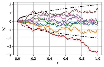
Var(W_t) at t=0.25: 0.2486   (theory: 0.25)
Var(W_t) at t=0.50: 0.4950   (theory: 0.50)
Var(W_t) at t=1.00: 1.0014   (theory: 1.00)
Var(W_t) at t=0.25: 0.2486   (theory: 0.25)
Var(W_t) at t=0.50: 0.4950   (theory: 0.50)
Var(W_t) at t=1.00: 1.0014   (theory: 1.00)
Var(W_t) at t=0.25: 0.2486   (theory: 0.25)
Var(W_t) at t=0.50: 0.4950   (theory: 0.50)
Var(W_t) at t=1.00: 1.0014   (theory: 1.00)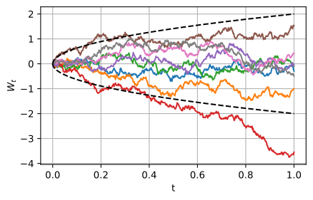
The empirical variances \(0.2486\), \(0.4950\), and \(1.0014\) match \(t\) within Monte Carlo error, and most plotted paths lie inside the square-root envelope. The covariance structure is just as checkable: the ensemble average of \(W_s W_t\) over a grid of time pairs should reproduce \(\min(s, t)\) entry by entry.
ts = np.array([0.1, 0.25, 0.5, 0.75, 1.0])
idx = np.round(ts / dt).astype(int)
emp = W[:, idx].T @ W[:, idx] / n_paths      # E[W_s W_t]; the means are zero
print('empirical E[W_s W_t]:')
print(emp.round(3))
print(f'max |empirical - min(s,t)| = {np.abs(emp - np.minimum.outer(ts, ts)).max():.4f}')
empirical E[W_s W_t]:
[[0.101 0.101 0.1 0.1 0.101]
[0.101 0.249 0.247 0.248 0.248]
[0.1 0.247 0.495 0.499 0.497]
[0.1 0.248 0.499 0.754 0.751]
[0.101 0.248 0.497 0.751 1.001]]
max |empirical - min(s,t)| = 0.0050The printed matrix matches \(\min(s, t)\) to within \(0.005\) in every entry, and it is constant along each row past the diagonal: increments after time \(s\) are uncorrelated with \(W_s\). Future increments are independent of the entire path so far; only the current position matters.
29.2.2 Itô Calculus
29.2.2.1 Quadratic Variation: Why Ordinary Calculus Fails
Quadratic variation distinguishes Brownian paths from smooth ones. Take a partition \(0 = t_0 < t_1 < \cdots < t_n = t\) with mesh \(\delta = \max_i \Delta t_i\), and ask what happens to the sum of squared increments of a function along it. For a continuously differentiable path \(x(t)\) the sum vanishes,
\[ \sum_{i} (\Delta x_i)^2 \;\le\; \max_i |\Delta x_i| \sum_i |\Delta x_i| \;\approx\; \delta \cdot \max|x'| \cdot \textrm{(total variation)} \;\longrightarrow\; 0, \]
which is precisely why Taylor expansions in ordinary calculus stop at first order: \((dx)^2\) is negligible against \(dx\). For Brownian motion the same sum has a nonzero limit: each \((\Delta W_i)^2\) has mean \(\Delta t_i\), and the means add up to exactly \(t\) no matter how fine the mesh (Figure 29.2.2).
Proposition (quadratic variation of Brownian motion). As the mesh \(\delta \to 0\),
\[ Q_n \;=\; \sum_{i=0}^{n-1} \left(W_{t_{i+1}} - W_{t_i}\right)^2 \;\longrightarrow\; t \quad \textrm{in mean square:} \quad \mathbb{E}\!\left[(Q_n - t)^2\right] \to 0. \tag{29.2.3}\]
Proof. Each increment is \(\mathcal{N}(0, \Delta t_i)\), so \(\mathbb{E}[(\Delta W_i)^2] = \Delta t_i\) and \(\mathbb{E}[Q_n] = \sum_i \Delta t_i = t\) exactly, for every partition. For the spread, a Gaussian has fourth moment \(3\,\Delta t_i^2\), so \(\operatorname{Var}\!\left((\Delta W_i)^2\right) = 3\Delta t_i^2 - \Delta t_i^2 = 2\Delta t_i^2\); the increments are independent, so their variances add:
\[ \mathbb{E}\!\left[(Q_n - t)^2\right] = \operatorname{Var}(Q_n) = \sum_i 2\,\Delta t_i^2 \;\le\; 2\,\delta \sum_i \Delta t_i = 2\,\delta\, t \;\longrightarrow\; 0, \]
and mean-square convergence follows. \(\blacksquare\)
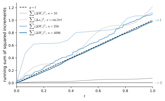
The sum of squared Brownian increments converges to the deterministic elapsed time. The proposition is usually compressed into the Itô multiplication table, the working rules for manipulating differentials:
\[ (dW)^2 = dt, \qquad dW\,dt = 0, \qquad (dt)^2 = 0. \tag{29.2.4}\]
The first rule is Equation 29.2.3 in shorthand; the other two record that \(dW\,dt \sim \Delta t^{3/2}\) and \((dt)^2 = \Delta t^2\) vanish faster than \(\Delta t\) and so contribute nothing in the limit. The following computation accumulates \(\sum (\Delta W_i)^2\) along one fixed Brownian path, sampled on finer and finer grids, and contrast it with the same sum for the smooth path \(\sin(2\pi t)\).
rng = np.random.default_rng(7)
T, n_fine = 1.0, 2**18
dW = np.sqrt(T / n_fine) * rng.standard_normal(n_fine)
W = np.concatenate([[0.0], np.cumsum(dW)])
print(f'{"n":>8} {"QV of W":>10} {"QV of sin(2 pi t)":>18}')
for k in range(4, 19, 2):
    n = 2**k
    Wn = W[::n_fine // n]                    # the same path on a coarser grid
    sn = np.sin(2 * np.pi * np.linspace(0, T, n + 1))
    print(f'{n:8d} {np.sum(np.diff(Wn)**2):10.4f} {np.sum(np.diff(sn)**2):18.6f}')
n QV of W QV of sin(2 pi t)
16 0.5575 1.217927
64 1.0456 0.308177
256 1.0245 0.077102
1024 1.0793 0.019277
4096 1.0308 0.004819
16384 1.0011 0.001205
65536 0.9950 0.000301
262144 0.9980 0.000075Read the two columns against the proposition. The Brownian column starts noisy (\(0.56\) on \(16\) intervals, where the proof predicts a standard deviation of \(\sqrt{2/n} \approx 0.35\) around the mean \(1\)) and converges to \(t = 1\) as the mesh shrinks (\(0.9980\) at \(n = 2^{18}\), where \(\sqrt{2/n} \approx 0.003\)). The smooth column collapses toward zero like \(1/n\), exactly as the differentiable-path estimate says. The smooth-path column converges to zero, whereas the Brownian column converges to elapsed time. This distinction requires stochastic calculus.
29.2.2.2 The Itô Integral
To give Equation 29.2.1 meaning, begin with a simple predictable process. On each interval \((t_i,t_{i+1}]\), let \(G_s=G_i\), where \(G_i\) is determined by the path through time \(t_i\) and \(\mathbb{E}[G_i^2]<\infty\). Define its Itô integral by
\[ \int_0^t G_s \, dW_s \;=\; \sum_i G_i\left(W_{t_{i+1}}-W_{t_i}\right). \tag{29.2.5}\]
Because \(G_i\) is fixed before the increment \(\Delta W_i\), independence gives \(\mathbb{E}[G_i\Delta W_i]=0\). The Itô isometry below makes this definition continuous in the norm \(\|G\|_{L^2}^2=\int_0^t\mathbb{E}[G_s^2]ds\). Simple predictable processes are dense among square-integrable predictable processes, so the integral extends uniquely by an \(L^2\) limit (Øksendal 2003). For sufficiently regular adapted \(G\), ordinary left-endpoint sums converge to this integral; arbitrary point samples are not the general definition.
First, the zero-mean property: \(\mathbb{E}\!\left[\int_0^t G\,dW\right] = 0\). The zero mean follows from choosing each coefficient before observing the corresponding increment. (A stronger fact holds, which we grant: given everything observed up to time \(s\), the expected future value of the integral equals its current value; processes with this fair-game property are called martingales (Øksendal 2003).) Second, its variance is computable:
Proposition (Itô isometry). For predictable \(G\) with \(\int_0^t \mathbb{E}[G_s^2]\,ds < \infty\),
\[ \mathbb{E}\!\left[\left(\int_0^t G_s\,dW_s\right)^{\!2}\,\right] \;=\; \int_0^t \mathbb{E}\!\left[G_s^2\right] ds. \tag{29.2.6}\]
Proof. First take a simple predictable \(G\) and expand the square of the sum in Equation 29.2.5. A cross term with \(i < j\) contains the factor \(\Delta W_j\), independent of everything determined by time \(t_j\) (including \(G_{t_i} \Delta W_i G_{t_j}\)), so it factorizes: \(\mathbb{E}\!\left[G_{t_i}\Delta W_i\, G_{t_j} \Delta W_j\right] = \mathbb{E}\!\left[G_{t_i}\Delta W_i\, G_{t_j}\right]\mathbb{E}[\Delta W_j] = 0\). A diagonal term factorizes the same way into \(\mathbb{E}\!\left[G_{t_i}^2\right]\mathbb{E}\!\left[(\Delta W_i)^2\right] = \mathbb{E}\!\left[G_i^2\right]\Delta t_i\). Summing the surviving diagonal gives \(\sum_i \mathbb{E}[G_i^2]\,\Delta t_i = \int_0^t \mathbb{E}[G_s^2]\,ds\). For a general square-integrable predictable \(G\), approximate it in \(L^2\) by simple predictable processes. Both sides converge by the defining norm, so the identity extends. \(\blacksquare\)
The isometry converts a stochastic computation (the variance of a noise integral) into an ordinary integral, and it is how we will obtain the Ornstein–Uhlenbeck variance in closed form below.
The evaluation point changes the stochastic integral. For a smooth integrator, left, right, and midpoint Riemann sums share one limit. Here they do not: evaluating at the right endpoint instead changes the sum by
\[ \sum_i \left(W_{t_{i+1}} - W_{t_i}\right)\Delta W_i = \sum_i (\Delta W_i)^2 \;\longrightarrow\; t, \]
the quadratic variation again: a finite, deterministic disagreement between two discretizations of “the same” integral. The midpoint choice defines the Stratonovich integral (Stratonovich 1966), which obeys the ordinary chain rule but gives up the zero-mean and fair-game properties; Itô’s left endpoint is the one that matches causal simulation (the integrand may not peek at the upcoming noise), which is why this book builds on it.
29.2.2.3 Itô’s Lemma
The Itô multiplication table determines the corresponding chain rule. Let \(X_t\) solve \(dX = f\,dt + g\,dW\) (made fully precise in Section 29.2.3; for now, read it through its increments) and let \(\phi(x, t)\) be once continuously differentiable in time and twice in state. Taylor-expand a small change of \(\phi\) to second order, since first order is no longer enough:
\[ d\phi = \phi_t\,dt + \phi_x\,dX + \tfrac12 \phi_{xx}\,(dX)^2 + \cdots. \]
Substitute \(dX = f\,dt + g\,dW\) and multiply out \((dX)^2\) using the table Equation 29.2.4:
\[ (dX)^2 = f^2 (dt)^2 + 2 f g\, dt\, dW + g^2 (dW)^2 = g^2\,dt. \]
The drift and cross terms vanish; the noise-squared term survives as a genuine first-order contribution. Collecting terms gives the central formula of the subject.
Proposition (Itô’s lemma). Suppose the SDE and the integrals below are well-defined, and let \(\phi\in C^{1,2}\): once continuously differentiable in time and twice in the state variable. Then \(Y_t=\phi(X_t,t)\) satisfies
\[ d\phi \;=\; \left(\phi_t + f\,\phi_x + \tfrac12 g^2\,\phi_{xx}\right) dt \;+\; g\,\phi_x \, dW. \tag{29.2.7}\]
The Taylor argument above is a heuristic; the full proof controls the error terms in mean square and can be found in Øksendal (2003), chapter 4. Relative to the ordinary chain rule, the additional term is \(\tfrac12 g^2 \phi_{xx}\,dt\), the Itô correction, which appears because \((dW)^2 = dt\). Curvature of \(\phi\) interacts with the jitter of \(X\): a convex \(\phi\) gains from symmetric noise (both wiggle directions push the value up), and the correction quantifies that gain. This single term seeds the \(\tfrac12 g^2 \partial_{xx}\) diffusion term of the Fokker–Planck equation in Section 29.3.
The multivariate form we also take as given, on the same authority (Øksendal 2003). For \(d\mathbf{X} = \mathbf{f}\,dt + G\,d\mathbf{W}\) with \(\mathbf{X} \in \mathbb{R}^d\), a matrix \(G\), and standard multivariate Brownian motion \(\mathbf{W}\), the multiplication table reads \((dW_i)(dW_j) = \delta_{ij}\,dt\), and a twice continuously differentiable \(\phi\) obeys
\[ d\phi(\mathbf{X}) \;=\; \nabla\phi \cdot d\mathbf{X} \;+\; \tfrac12 \sum_{i,j} \left(G G^\top\right)_{ij} \partial^2_{x_i x_j}\phi \; dt . \tag{29.2.8}\]
For the diagonal, state-independent noise \(G = g(t)\,I\) that every SDE in this chapter uses, \(G G^\top = g(t)^2 I\) and the correction collapses to the single Laplacian term \(\tfrac12 g(t)^2\,\Delta\phi\,dt\), where \(\Delta\phi = \sum_i \partial^2_{x_i x_i}\phi\).
The canonical check is \(\phi(x) = x^2\) applied to \(X = W\) itself (so \(f = 0\), \(g = 1\)): the lemma gives \(d(W^2) = 2W\,dW + dt\), and the naive chain rule would have dropped the \(dt\). In integrated form,
\[ W_t^2 = \int_0^t 2 W_s \, dW_s + t, \qquad\textrm{i.e.}\qquad \int_0^t W_s\,dW_s = \tfrac12\left(W_t^2 - t\right), \tag{29.2.9}\]
where the \(-t\) is forced by consistency: the left-endpoint integral has mean zero while \(\mathbb{E}[W_t^2] = t\), so the ordinary-calculus answer \(\tfrac12 W_t^2\) cannot be right. The correction is large enough to see on a single simulated path: we accumulate the left-endpoint sum \(\int_0^t 2W\,dW\) and plot its gap to \(W_t^2\).
rng = np.random.default_rng(3)
T, n = 1.0, 1000
dt = T / n
t = np.linspace(0, T, n + 1)
dW = np.sqrt(dt) * rng.standard_normal(n)
W = np.concatenate([[0.0], np.cumsum(dW)])
ito = np.concatenate([[0.0], np.cumsum(2 * W[:-1] * dW)])    # left endpoint
print(f'W_T^2 - int 2W dW = {W[-1]**2 - ito[-1]:.4f}   (Ito correction: T = {T})')
print(f'max |gap_t - t| along the path = {np.abs(W**2 - ito - t).max():.4f}')
d2l.plot(t, [W**2, ito, ito + t], 't', 'value',
         legend=['$W_t^2$', 'naive $\\int_0^t 2W\\,dW$', '$\\int_0^t 2W\\,dW + t$'],
figsize=(5, 3))W_T^2 - int 2W dW = 1.0150 (Ito correction: T = 1.0)
max |gap_t - t| along the path = 0.0235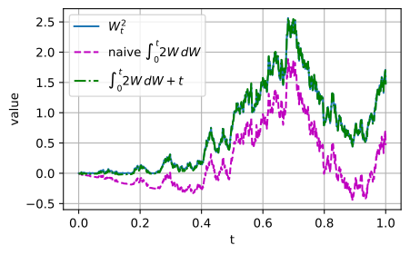
W_T^2 - int 2W dW = 1.0150   (Ito correction: T = 1.0)
max |gap_t - t| along the path = 0.0235
W_T^2 - int 2W dW = 1.0150   (Ito correction: T = 1.0)
max |gap_t - t| along the path = 0.0235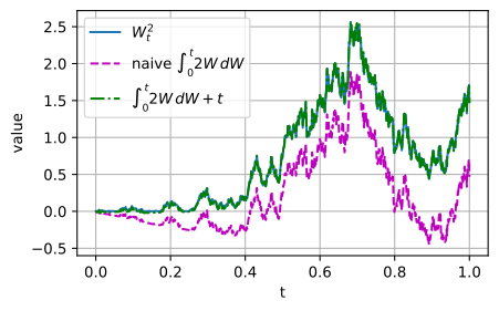
W_T^2 - int 2W dW = 1.0150   (Ito correction: T = 1.0)
max |gap_t - t| along the path = 0.0235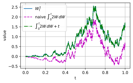
The final gap is \(1.0150\) against the predicted \(T = 1\), and along the whole path the gap never strays more than \(0.024\) from \(t\), because the gap at time \(t\) is exactly the accumulated quadratic variation \(\sum_{t_i \le t} (\Delta W_i)^2\), which Equation 29.2.3 pins to \(t\). The naive curve \(\int 2W\,dW\) visibly sags below \(W_t^2\); adding back \(t\) locks the two together. The Itô correction is a unit-slope drift you can plot.
29.2.3 Stochastic Differential Equations and Euler–Maruyama
29.2.3.1 Drift, Diffusion, and What a Solution Is
The preceding definitions specify a stochastic differential equation. A stochastic differential equation is
\[ dX = f(X, t)\,dt + g(X, t)\,dW, \tag{29.2.10}\]
shorthand (since \(dW/dt\) does not exist, the differential form is defined through its integrated meaning) for
\[ X_t = X_0 + \int_0^t f(X_s, s)\,ds + \int_0^t g(X_s, s)\,dW_s, \]
an ordinary integral plus an Itô integral. The drift \(f\) steers the average motion and the diffusion \(g\) injects Brownian jitter: over a short step, \(\mathbb{E}[dX] = f\,dt\) while \(\operatorname{Var}(dX) = g^2\,dt\), so \(f\) is the conditional mean velocity and \(g^2\) the rate at which variance is pumped in. Setting \(g \equiv 0\) recovers the deterministic ODE of Section 29.1 exactly. As with ODEs, Lipschitz continuity of \(f\) and \(g\) (in \(x\), with at most linear growth) guarantees a unique strong solution up to indistinguishability: the stochastic Picard iteration of Øksendal (2003), chapter 5, mirrors the deterministic one of Section 29.1.1.3.
Diffusion models use the special case in which the noise amplitude depends on time but not on state, \(dX = f(X, t)\,dt + g(t)\,dW\): additive noise, the template Equation 29.2.1. The distinction between additive \(g(t)\) and the general state-dependent multiplicative \(g(X, t)\) looks cosmetic but will decide the accuracy of our numerical scheme below. The two standard noising families are both additive: variance-exploding (zero drift, growing \(g\), so the data is buried under ever-larger noise) and variance-preserving (a restoring drift balanced against the noise, the Ornstein–Uhlenbeck design we build in Section 29.2.4 and reuse in Section 29.4).
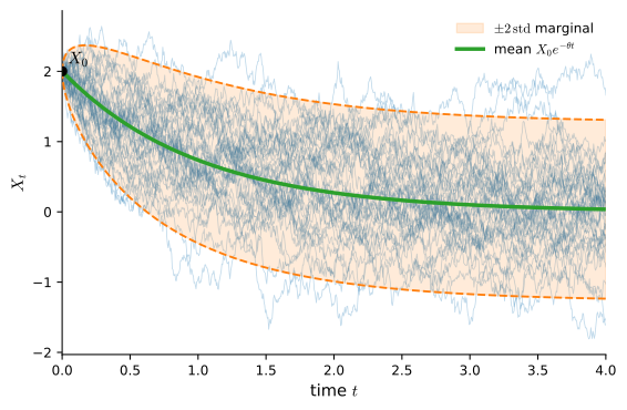
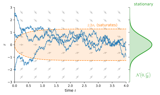
Unlike an ODE solution, an SDE solution is a stochastic process whose law is a distribution over paths rather than a single curve. Fixing \(X_0\) and running Equation 29.2.10 many times with fresh noise produces a fan of jittery trajectories whose ensemble statistics, the time marginals \(p_t\), are what generative modeling cares about. Figure 29.2.3 shows this fan for the Ornstein–Uhlenbeck process: the mean follows the drift, the spread is set by the diffusion, and the envelope saturates as the initial condition’s influence decays. Section 29.3 turns this picture into an equation for \(p_t\) itself.
29.2.3.2 The Euler–Maruyama Scheme
To simulate Equation 29.2.10 we discretize it exactly as we discretized ODEs in Section 29.1.3 (freeze the coefficients over each step), plus one new ingredient: a Gaussian noise kick whose size is dictated by Equation 29.2.2. The Euler–Maruyama (EM) update (Maruyama 1955) reads
\[ X_{n+1} = X_n + f(X_n, t_n)\,\Delta t + g(X_n, t_n)\,\sqrt{\Delta t}\;\xi_n, \qquad \xi_n \sim \mathcal{N}(0, 1) \textrm{ i.i.d.} \tag{29.2.11}\]
The noise scales as \(\sqrt{\Delta t}\), never \(\Delta t\): the kick is a Brownian increment over the step, and we saw in Section 29.2.1.2 that any other exponent makes the noise vanish or explode in the limit. When \(g = 0\) the scheme is forward Euler. The helper below implements Equation 29.2.11 for a whole batch of paths at once, and the sanity check runs it with \(g = 0\) on \(\dot{x} = -x\).
def euler_maruyama(f, g, x0, t, dW):
    """Simulate dX = f dt + g dW on the grid t for a batch of paths."""
    X = np.empty((len(x0), len(t)))
    X[:, 0] = x0
    for k in range(len(t) - 1):
        h = t[k + 1] - t[k]
        X[:, k + 1] = X[:, k] + f(X[:, k], t[k]) * h + g(X[:, k], t[k]) * dW[:, k]
    return X

t = np.linspace(0, 2.0, 201)
X = euler_maruyama(lambda x, s: -x, lambda x, s: 0.0,
                   np.ones(1), t, np.zeros((1, 200)))
print('g = 0 recovers Euler on dx/dt = -x: '
      f'max |X_t - e^(-t)| = {np.abs(X[0] - np.exp(-t)).max():.5f}')
g = 0 recovers Euler on dx/dt = -x: max |X_t - e^(-t)| = 0.00185With the noise switched off we are back to the familiar first-order Euler error (\(1.9 \times 10^{-3}\) at \(h = 10^{-2}\)). With the noise switched on, “error” itself needs a definition, and it splits in two.
29.2.3.3 Strong and Weak Convergence
Fix one Brownian path and feed the same increments to the exact solution and to the scheme. The strong error \(\mathbb{E}\,|X^{\Delta t}_N - X_T|\) measures pathwise tracking: does the simulated trajectory follow the true trajectory driven by that noise? The weak error \(|\mathbb{E}\,\varphi(X^{\Delta t}_N) - \mathbb{E}\,\varphi(X_T)|\), for smooth test functions \(\varphi\), measures distributional accuracy: do the marginals come out right, even if individual paths wander? Weak error is the direct criterion for endpoint-law sampling. Strong error remains relevant when an application couples trajectories across resolutions, reconstructs a fixed latent path, or differentiates through a particular numerical realization. Figure 29.2.4 shows the two notions side by side. The classical rates (Kloeden and Platen 1992) are:
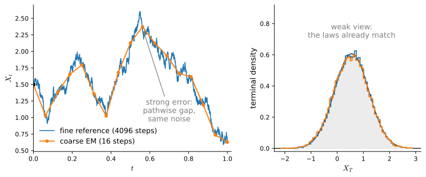
Proposition (strong order of Euler–Maruyama). Under global Lipschitz and linear-growth conditions on \(f\) and \(g\), Euler–Maruyama has strong order \(\tfrac12\) in general: \(\mathbb{E}\,|X^{\Delta t}_N - X_T| \le C\,\Delta t^{1/2}\). For additive noise, \(g=g(t)\), the rate improves to strong order \(1\) provided the coefficients have the additional time regularity and bounded derivatives required by the stochastic Taylor estimate: \(\mathbb{E}\,|X^{\Delta t}_N - X_T| \le C\,\Delta t\).
Proposition (weak order of Euler–Maruyama). If \(f\), \(g\), and the test function \(\varphi\) have sufficiently many derivatives (with the usual growth bounds), Euler–Maruyama has weak order \(1\): \(|\mathbb{E}\,\varphi(X^{\Delta t}_N) - \mathbb{E}\,\varphi(X_T)| \le C\,\Delta t\), additive or not.
We do not prove these; the intuition for the strong-order gap is the multiplication table again. EM is the stochastic Taylor expansion of the solution truncated after the \(g\,\Delta W\) term; the first omitted term is Milstein’s \(\tfrac12 g\, \partial_x g\,\left((\Delta W)^2 - \Delta t\right)\) (Milstein 1975). Per step this is mean-zero with standard deviation proportional to \(\Delta t\), and summing \(1/\Delta t\) independent mean-zero terms grows their total like a random walk: \(\Delta t \cdot \sqrt{1/\Delta t} = \sqrt{\Delta t}\), the order \(\tfrac12\). For additive noise \(\partial_x g = 0\) makes the Milstein term vanish identically. Under the extra smoothness just stated, the remaining terms accumulate to a global \(O(\Delta t)\) strong error. With sufficiently smooth test functions and coefficients, the leading mean-zero terms cancel in expectation, leaving \(O(\Delta t)\) weak bias.
Every SDE treated numerically in this chapter (Ornstein–Uhlenbeck and the two diffusion-model families) has smooth additive noise, so strong order \(1\) is the relevant prediction for these examples rather than the general \(\tfrac12\) rate. Let us measure both rates in one experiment: the OU process \(dX = -\theta X\,dt + \sigma\,dW\) (additive; compare against a fine-grid reference driven by the same increments) and geometric Brownian motion \(dX = \mu X\,dt + \sigma X\,dW\) (Black and Scholes 1973) (multiplicative; compare against its exact solution \(X_T = X_0 \exp\!\left((\mu - \tfrac{\sigma^2}{2})T + \sigma W_T\right)\), which you will derive via Itô’s lemma in Exercise 5).
rng = np.random.default_rng(0)
T, X0, n_fine, n_paths = 1.0, 1.5, 2**12, 2000
theta, sigma = 1.0, 1.0                      # OU: additive noise
mu_g, sig_g = 1.0, 1.0                       # GBM: multiplicative noise
dW_f = np.sqrt(T / n_fine) * rng.standard_normal((n_paths, n_fine))
t_f = np.linspace(0, T, n_fine + 1)
x0 = np.full(n_paths, X0)
ou_ref = euler_maruyama(lambda x, s: -theta * x, lambda x, s: sigma,
                        x0, t_f, dW_f)[:, -1]
gbm_exact = X0 * np.exp((mu_g - sig_g**2 / 2) * T + sig_g * dW_f.sum(axis=1))
dts, errs_ou, errs_gbm = [], [], []
for n in [2**k for k in range(3, 9)]:        # 8 to 256 steps
    dW = dW_f.reshape(n_paths, n, n_fine // n).sum(axis=2)
    t = np.linspace(0, T, n + 1)
    ou = euler_maruyama(lambda x, s: -theta * x, lambda x, s: sigma, x0, t, dW)
    gbm = euler_maruyama(lambda x, s: mu_g * x, lambda x, s: sig_g * x, x0, t, dW)
    dts.append(T / n)
    errs_ou.append(np.abs(ou[:, -1] - ou_ref).mean())
    errs_gbm.append(np.abs(gbm[:, -1] - gbm_exact).mean())
print('strong-order slopes:  OU (additive) '
      f'{np.polyfit(np.log(dts), np.log(errs_ou), 1)[0]:.2f},'
      '  GBM (multiplicative) '
      f'{np.polyfit(np.log(dts), np.log(errs_gbm), 1)[0]:.2f}')
d2l.plot(dts, [errs_ou, errs_gbm, np.array(dts), 0.5 * np.sqrt(dts)],
         'step size', 'strong error', xscale='log', yscale='log',
         legend=['OU (additive)', 'GBM (multiplicative)',
'slope 1', 'slope 1/2'], figsize=(5, 3))strong-order slopes: OU (additive) 1.02, GBM (multiplicative) 0.45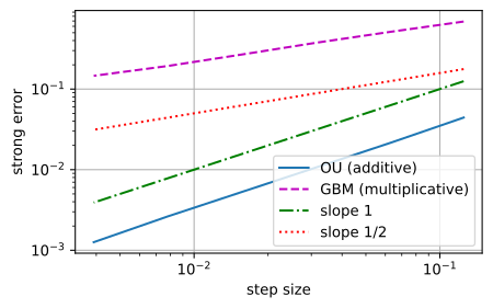
strong-order slopes: OU (additive) 1.02, GBM (multiplicative) 0.45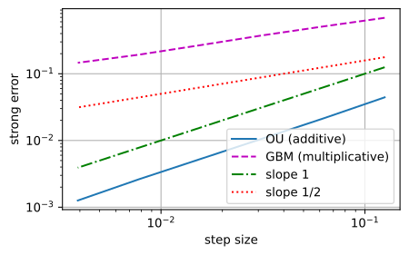
strong-order slopes: OU (additive) 1.02, GBM (multiplicative) 0.45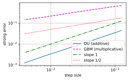
strong-order slopes: OU (additive) 1.02, GBM (multiplicative) 0.45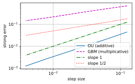
The measured slopes are \(1.02\) for the additive-noise OU process and \(0.45\) for multiplicative-noise GBM: the two propositions, confirmed side by side on the same Brownian increments. On the log–log plot the OU error follows the slope-\(1\) guide while GBM follows the slope-\(\tfrac12\) guide; at \(\Delta t = 2^{-8}\) the additive problem is already two orders of magnitude more accurate.
For the weak rate, no sampling is needed. EM applied to OU is a linear Gaussian recursion (if \(X_n\) is Gaussian then so is \(X_{n+1}\)), so the simulated marginal stays exactly Gaussian, with mean and variance obeying
\[ m_{n+1} = (1 - \theta\,\Delta t)\,m_n, \qquad v_{n+1} = (1 - \theta\,\Delta t)^2\, v_n + \sigma^2\,\Delta t . \]
Both recursions close in elementary form, so the weak error of the entire marginal reduces to two numbers we can evaluate to machine precision, with no sampling noise contaminating the measured slope.
theta, sigma, T, X0 = 1.0, 1.0, 1.0, 1.5
mean_T = X0 * np.exp(-theta * T)
var_T = sigma**2 / (2 * theta) * (1 - np.exp(-2 * theta * T))
dts, errs = [], []
for n in [10, 20, 40, 80, 160, 320]:
    h = T / n
    a = 1 - theta * h                        # one-step mean multiplier
    m = X0 * a**n                            # EM mean after n steps
    v = sigma**2 * h * (1 - a**(2 * n)) / (1 - a**2)   # EM variance
    dts.append(h)
    errs.append([abs(m - mean_T), abs(v - var_T)])
sm, sv = np.polyfit(np.log(dts), np.log(np.array(errs)), 1)[0]
print(f'weak-order slopes on OU:  mean {sm:.2f},  variance {sv:.2f}')
weak-order slopes on OU: mean 1.01, variance 1.01The slopes are \(1.01\) for both the mean and variance errors, consistent with weak order \(1\). (The exact OU mean and variance used as ground truth here are derived in the next section.) Halving the step halves the marginal error: the rate at which a discretized diffusion model’s forward marginals approach the SDE’s, a fact Section 29.4.2.2 leans on when it reads DDPM’s forward chain as exactly this discretization.
29.2.4 The Ornstein–Uhlenbeck Process
The Ornstein–Uhlenbeck process (Uhlenbeck and Ornstein 1930) is
\[ dX = -\theta X \, dt + \sigma\,dW, \qquad \theta > 0. \tag{29.2.12}\]
The drift is the stable linear ODE of Section 29.1.2 (\(\dot{x} = -\theta x\), exponential decay toward the origin) with Brownian noise of constant amplitude \(\sigma\) added. The mean-reverting drift pulls excursions toward zero at rate \(\theta\), while the noise continually introduces new variation. The resulting process (Figure 29.2.5) has a closed-form transition law and therefore provides a convenient basis for variance-preserving diffusion.
29.2.4.1 Solving the SDE with Itô’s Lemma
We use the same integrating factor that solves the deterministic equation. Apply Itô’s lemma Equation 29.2.7 to \(\phi(x, t) = e^{\theta t} x\), for which \(\phi_t = \theta e^{\theta t} x\), \(\phi_x = e^{\theta t}\), and \(\phi_{xx} = 0\), so the Itô correction vanishes (knowing when the correction is zero is as useful as knowing its value):
\[ d\!\left(e^{\theta t} X_t\right) = \left(\theta e^{\theta t} X_t - \theta e^{\theta t} X_t\right) dt + e^{\theta t}\sigma\,dW_t = \sigma\, e^{\theta t}\,dW_t. \]
The drift cancels exactly; what remains integrates immediately to
\[ X_t = X_0\, e^{-\theta t} + \sigma \int_0^t e^{-\theta (t - s)}\, dW_s . \tag{29.2.13}\]
Read it as a fading memory: the start \(X_0\) decays at rate \(\theta\), and each past noise kick \(dW_s\) persists with weight \(e^{-\theta(t-s)}\); recent noise counts, ancient noise is forgotten. The remaining integral has a deterministic integrand, so it is a limit of weighted sums of independent Gaussians, hence Gaussian itself (we grant that mean-square limits of Gaussian random variables are Gaussian); its mean is zero, and the Itô isometry Equation 29.2.6 computes its variance as an ordinary integral:
\[ \operatorname{Var}(X_t \mid X_0) = \sigma^2 \int_0^t e^{-2\theta (t - s)}\, ds = \frac{\sigma^2}{2\theta}\left(1 - e^{-2\theta t}\right). \]
Proposition (OU transition kernel). For the OU process Equation 29.2.12,
\[ X_t \mid X_0 = x_0 \;\sim\; \mathcal{N}\!\left( x_0\, e^{-\theta t},\; \frac{\sigma^2}{2\theta}\left(1 - e^{-2\theta t}\right) \right). \tag{29.2.14}\]
A closed-form Gaussian at every time, for every start: this is the Gaussian noising kernel that lets denoising score matching evaluate its regression target in closed form (Section 29.4.1.2). The following Euler–Maruyama simulation compares the kernel with an ensemble launched from the single point \(X_0 = 2\) (matching Figure 29.2.3), with the analytic mean and \(\pm 2\sigma_t\) band overlaid.
rng = np.random.default_rng(1)
theta, sigma, X0, T, n, n_paths = 1.0, 0.9, 2.0, 4.0, 800, 10000
t = np.linspace(0, T, n + 1)
dW = np.sqrt(T / n) * rng.standard_normal((n_paths, n))
X = euler_maruyama(lambda x, s: -theta * x, lambda x, s: sigma,
                   np.full(n_paths, X0), t, dW)
mean_th = X0 * np.exp(-theta * t)
std_th = np.sqrt(sigma**2 / (2 * theta) * (1 - np.exp(-2 * theta * t)))
for s in [0.5, 1.0, 2.0, 4.0]:
    k = round(s / (T / n))
    print(f't={s:.1f}:  mean {X[:, k].mean():7.4f} vs {mean_th[k]:7.4f},   '
          f'std {X[:, k].std():.4f} vs {std_th[k]:.4f}')
inside = np.abs(X[:, -1] - mean_th[-1]) < 2 * std_th[-1]
print(f'fraction of paths inside the +-2 sigma band at t={T:.0f}: '
      f'{inside.mean():.3f}   (Gaussian: 0.954)')
d2l.plot(t, [X[i] for i in range(6)]
         + [mean_th, mean_th + 2 * std_th, mean_th - 2 * std_th],
't', '$X_t$', fmts=['-'] * 6 + ['k-', 'k--', 'k--'], figsize=(5, 3))t=0.5: mean 1.2237 vs 1.2131, std 0.4997 vs 0.5060
t=1.0: mean 0.7336 vs 0.7358, std 0.5912 vs 0.5918
t=2.0: mean 0.2712 vs 0.2707, std 0.6304 vs 0.6305
t=4.0: mean 0.0406 vs 0.0366, std 0.6399 vs 0.6363
fraction of paths inside the +-2 sigma band at t=4: 0.952 (Gaussian: 0.954)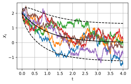
t=0.5:  mean  1.2237 vs  1.2131,   std 0.4997 vs 0.5060
t=1.0:  mean  0.7336 vs  0.7358,   std 0.5912 vs 0.5918
t=2.0:  mean  0.2712 vs  0.2707,   std 0.6304 vs 0.6305
t=4.0:  mean  0.0406 vs  0.0366,   std 0.6399 vs 0.6363
fraction of paths inside the +-2 sigma band at t=4: 0.952   (Gaussian: 0.954)
t=0.5:  mean  1.2237 vs  1.2131,   std 0.4997 vs 0.5060
t=1.0:  mean  0.7336 vs  0.7358,   std 0.5912 vs 0.5918
t=2.0:  mean  0.2712 vs  0.2707,   std 0.6304 vs 0.6305
t=4.0:  mean  0.0406 vs  0.0366,   std 0.6399 vs 0.6363
fraction of paths inside the +-2 sigma band at t=4: 0.952   (Gaussian: 0.954)
t=0.5:  mean  1.2237 vs  1.2131,   std 0.4997 vs 0.5060
t=1.0:  mean  0.7336 vs  0.7358,   std 0.5912 vs 0.5918
t=2.0:  mean  0.2712 vs  0.2707,   std 0.6304 vs 0.6305
t=4.0:  mean  0.0406 vs  0.0366,   std 0.6399 vs 0.6363
fraction of paths inside the +-2 sigma band at t=4: 0.952   (Gaussian: 0.954)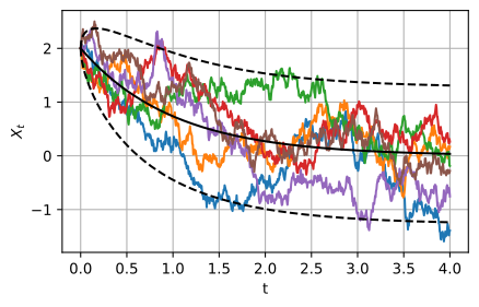
Simulation and kernel agree to Monte-Carlo precision: at \(t = 1\) the ensemble mean is \(0.7336\) against the analytic \(0.7358\) and the standard deviation \(0.5912\) against \(0.5918\), and \(95.2\%\) of paths sit inside the \(\pm 2\sigma_t\) band at \(t = 4\), matching the Gaussian \(95.4\%\). The band’s half-width grows and then saturates, which brings us to where the process ends up.
29.2.4.2 The Stationary Distribution
Send \(t \to \infty\) in the kernel Equation 29.2.14: the mean \(x_0 e^{-\theta t}\) decays and the variance approaches the limit \(\sigma^2\!/(2\theta)\), leaving
\[ X_\infty \sim \mathcal{N}\!\left(0, \, \frac{\sigma^2}{2\theta}\right) \]
regardless of \(x_0\): the process forgets its initial condition entirely, which is exactly the “known, distribution-independent endpoint” that Section 29.2.1.1 demanded of a forward noising process. The limit is stationary in the strong sense that it is invariant: if \(X_0 \sim \mathcal{N}(0, \sigma^2\!/2\theta)\) is drawn independently of the driving noise \(W\), then for every later \(t\), combining the decayed start with the accumulated noise gives variance
\[ e^{-2\theta t}\,\frac{\sigma^2}{2\theta} + \frac{\sigma^2}{2\theta}\left(1 - e^{-2\theta t}\right) = \frac{\sigma^2}{2\theta}, \]
while the mean stays zero; and since Equation 29.2.13 writes \(X_t\) as a sum of independent Gaussians, \(X_t\) is Gaussian with these moments, hence equal in law to \(X_0\). Relaxation toward stationarity happens on the time scale \(1/\theta\): after a few multiples, \(e^{-\theta t}\) is negligible. At \(t = 4\) (four relaxation times, for our \(\theta = 1\)) the ensemble from the previous cell should already be close to the stationary Gaussian, even though every path started from the same point \(2\).
var_inf = sigma**2 / (2 * theta)
samples = X[:, -1]                           # t = 4 is four relaxation times
print(f'ensemble variance at t=4: {samples.var():.4f}   '
      f'(stationary sigma^2/(2 theta) = {var_inf:.4f})')
xs = np.linspace(-2.5, 2.5, 201)
density = np.exp(-xs**2 / (2 * var_inf)) / np.sqrt(2 * np.pi * var_inf)
d2l.set_figsize((5, 3))
d2l.plt.hist(samples, bins=60, density=True, alpha=0.5,
             label='ensemble at $t=4$')
d2l.plt.plot(xs, density, 'k', label='stationary density')
d2l.plt.xlabel('$x$')
d2l.plt.legend()
d2l.plt.show()ensemble variance at t=4: 0.4095 (stationary sigma^2/(2 theta) = 0.4050)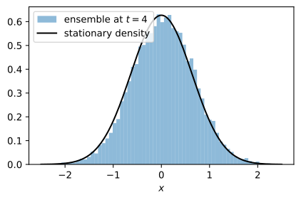
ensemble variance at t=4: 0.4095 (stationary sigma^2/(2 theta) = 0.4050)
ensemble variance at t=4: 0.4095 (stationary sigma^2/(2 theta) = 0.4050)
ensemble variance at t=4: 0.4095 (stationary sigma^2/(2 theta) = 0.4050)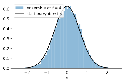
The histogram lies on the analytic density, with empirical variance \(0.4095\) against \(\sigma^2\!/(2\theta) = 0.405\). (Decompose the leftover half-percent. EM’s weak-order-\(1\) bias is computable exactly here: the variance recursion of #sdes-em-weak-order has fixed point \(\sigma^2 \Delta t / \left(1 - (1 - \theta \Delta t)^2\right) = 0.4060\) at \(\Delta t = 5 \times 10^{-3}\), so discretization explains only \(+0.001\) of the \(+0.0045\) gap. The Monte-Carlo standard error of a \(10{,}000\)-sample variance is \(\approx 0.006\); the rest, indeed most, of the gap is statistics, sitting on top of a small deterministic bias.) Mean reversion has converted a point mass into a distribution close to the stationary Gaussian.
29.2.4.3 The Variance-Preserving Normalization
Diffusion models select the remaining parameter by setting
\[ \sigma^2 = 2\theta \qquad \Longrightarrow \qquad X_\infty \sim \mathcal{N}(0, 1), \]
a unit-variance endpoint. With this normalization, abbreviate the squared decay factor as \(\bar{\alpha}_t = e^{-2\theta t}\); the solution Equation 29.2.13 says that in distribution
\[ X_t \;=\; \sqrt{\bar{\alpha}_t}\; X_0 \;+\; \sqrt{1 - \bar{\alpha}_t}\; \boldsymbol{\epsilon}, \qquad \boldsymbol{\epsilon} \sim \mathcal{N}(0, 1) \textrm{ independent of } X_0, \tag{29.2.15}\]
which has the same form as the DDPM forward marginal (Ho et al. 2020), with \(\bar{\alpha}_t\) playing its usual role. Now suppose the data is normalized to zero mean and unit variance (standard practice, and the next display is why). Taking variances in Equation 29.2.15, with \(X_0\) and \(\boldsymbol{\epsilon}\) independent:
\[ \operatorname{Var}(X_t) = \bar{\alpha}_t \operatorname{Var}(X_0) + (1 - \bar{\alpha}_t) = \bar{\alpha}_t + (1 - \bar{\alpha}_t) = 1 \qquad \textrm{for all } t. \]
This is what variance-preserving (VP) means: given unit-variance data, the marginal variance equals \(1\) exactly, at every time. The \(t \to \infty\) statement is strictly weaker, as is the observation that drift balances diffusion at stationarity (true of any process that has a stationary distribution). The forward process reallocates the variance (a fraction \(\bar{\alpha}_t\) still carried by the data, the complementary \(1 - \bar{\alpha}_t\) already replaced by noise) without ever changing the total. Higher moments and the distribution’s shape still change as the law approaches the Gaussian. We demonstrate this with data as non-Gaussian as possible at unit variance, the two-point (Rademacher) distribution \(X_0 = \pm 1\), and track two moments: the variance, which should stay pinned at \(1\), and the fourth moment \(\mathbb{E}[X_t^4]\), which Equation 29.2.15 predicts to be \(3 - 2\bar{\alpha}_t^2\) (Exercise 8), changing from the bimodal value \(1\) to the Gaussian value \(3\).
rng = np.random.default_rng(2)
theta = 1.0
sigma = np.sqrt(2 * theta)                   # the VP choice: sigma^2 = 2 theta
T, n, n_paths = 3.0, 300, 50000
t = np.linspace(0, T, n + 1)
x0 = rng.choice([-1.0, 1.0], size=n_paths)   # unit-variance, far from Gaussian
dW = np.sqrt(T / n) * rng.standard_normal((n_paths, n))
X = euler_maruyama(lambda x, s: -theta * x, lambda x, s: sigma, x0, t, dW)
print(f'{"t":>5} {"Var(X_t)":>9} {"E[X_t^4]":>9} {"3 - 2 alpha_t^2":>16}')
for s in [0.0, 0.25, 1.0, 3.0]:
    k = round(s / (T / n))
    alpha = np.exp(-2 * theta * s)
    print(f'{s:5.2f} {X[:, k].var():9.4f} {np.mean(X[:, k]**4):9.3f} '
          f'{3 - 2 * alpha**2:16.3f}')
t Var(X_t) E[X_t^4] 3 - 2 alpha_t^2
0.00 1.0000 1.000 1.000
0.25 1.0030 2.286 2.264
1.00 1.0073 2.999 2.963
3.00 1.0139 3.062 3.000The variance column reads \(1.000\), \(1.003\), \(1.007\), \(1.014\) (pinned at \(1\) up to EM bias) while the fourth moment changes from \(1.000\) through \(2.286\) (analytic \(2.264\)) to \(3.06\) against the Gaussian \(3\). The overshoot is mostly EM’s weak bias: the printed variance \(1.014\) corresponds to a Gaussian fourth moment of \(3v^2 \approx 3.08\), and the remainder sits inside one Monte-Carlo standard error (\(\approx 0.04\) for a fourth moment on \(50{,}000\) paths). The distribution is close to Gaussian, while the variance remains near one. Time-dependent noise schedules are a direct generalization: the VP-SDE of score-based diffusion (Song et al. 2021),
\[ dX = -\tfrac12 \beta(t)\, X \, dt + \sqrt{\beta(t)}\; dW, \tag{29.2.16}\]
is an OU process with time-rescaled rate \(\theta(t) = \beta(t)/2\) and noise \(\sigma(t)^2 = \beta(t)\), which satisfies \(\sigma(t)^2 = 2\,\theta(t)\) at every instant: the unit-variance normalization, maintained along the whole schedule (with \(\bar{\alpha}_t = e^{-\int_0^t \beta(s)\,ds}\) replacing \(e^{-2\theta t}\)). This SDE supplies the forward marginals used below: its marginals solve the Fokker–Planck equation of Section 29.3, its time reversal is the generative sampler of Section 29.3.5, and its Euler–Maruyama discretization gives the first-order continuous-time approximation behind DDPM’s forward chain (Section 29.4.2.2). The discrete DDPM coefficients are chosen so that each finite Gaussian transition is exact; they are not simply an Euler–Maruyama step with identical coefficients.
29.2.5 Summary
- Randomness makes the standard forward noising process useful in generative modeling: under an appropriate long-time schedule it drives a broad class of data distributions toward a known Gaussian reference. At finite time the endpoint is generally only approximately Gaussian.
- Brownian motion is the \(\pm\sqrt{\Delta t}\) random walk’s limit: independent Gaussian increments, \(W_t - W_s \sim \mathcal{N}(0, t-s)\), \(\operatorname{Var}(W_t) = t\), \(\operatorname{Cov}(W_s, W_t) = \min(s,t)\). Paths are continuous but nowhere differentiable: increments of size \(\sqrt{\Delta t}\) make \(\Delta W / \Delta t\) diverge.
- Quadratic variation: \(\sum (\Delta W_i)^2 \to t\) in mean square; squared noise accumulates deterministically. In differential shorthand, \((dW)^2 = dt\), \(dW\,dt = 0\), \((dt)^2 = 0\).
- The Itô integral is defined first for predictable simple processes and extended by an \(L^2\) limit. Predictability yields zero mean and the isometry \(\mathbb{E}[(\int G\,dW)^2] = \int \mathbb{E}[G^2]\,ds\). Itô’s lemma is the chain rule plus the correction \(\tfrac12 g^2 \phi_{xx}\,dt\) forced by \((dW)^2 = dt\); on \(\phi = W^2\) the correction is the visible \(+t\) in \(W_t^2 = \int 2W\,dW + t\).
- An SDE \(dX = f\,dt + g\,dW\) is drift (mean velocity) plus diffusion (variance injection); \(g = 0\) recovers the ODE, and a solution is a distribution over paths. Euler–Maruyama is forward Euler plus a \(\sqrt{\Delta t}\) Gaussian kick: under standard regularity assumptions it has strong order \(\tfrac12\) for general multiplicative noise, strong order \(1\) for sufficiently smooth additive-noise problems, and weak order \(1\) for sufficiently smooth coefficients and test functions. Weak (marginal) accuracy is what diffusion models usually need.
- The Ornstein–Uhlenbeck process \(dX = -\theta X\,dt + \sigma\,dW\) solves in closed form: Gaussian transition kernel \(\mathcal{N}\!\left(x_0 e^{-\theta t}, \tfrac{\sigma^2}{2\theta}(1 - e^{-2\theta t})\right)\), stationary law \(\mathcal{N}(0, \sigma^2\!/2\theta)\) approached from any start.
- With \(\sigma^2 = 2\theta\) and unit-variance data, the marginal is \(X_t = \sqrt{\bar{\alpha}_t} X_0 + \sqrt{1 - \bar{\alpha}_t}\,\epsilon\) and \(\operatorname{Var}(X_t) = \bar{\alpha}_t + (1 - \bar{\alpha}_t) = 1\) for all \(t\): the exact meaning of variance-preserving, and the DDPM forward marginal in continuous time.
29.2.6 Exercises
- The square-root scaling is forced. For the random walk with step duration \(\Delta t\) and step size \(c\,(\Delta t)^{\gamma}\), compute \(\operatorname{Var}(W^{(\Delta t)}_t)\) for fixed \(t\) and show that the limit as \(\Delta t \to 0\) is \(0\) for \(\gamma > \tfrac12\), \(\infty\) for \(\gamma < \tfrac12\), and \(c^2 t\) for \(\gamma = \tfrac12\). Conclude that Brownian motion is the only nontrivial scaling limit in this family.
- No velocity. Using \(W_{t+\Delta t} - W_t \sim \sqrt{\Delta t}\,\xi\), show that \(\mathbb{P}\left(\left|\Delta W / \Delta t\right| > M\right) \to 1\) as \(\Delta t \to 0\) for every fixed \(M\). Why does this rule out defining an SDE pathwise as \(\dot{X} = f + g\,\dot{W}\), and how does the integral formulation sidestep the problem?
- Quadratic variation, by hand and by machine. Re-derive \(\mathbb{E}[Q_n] = t\) and \(\operatorname{Var}(Q_n) \le 2\delta t\) without looking. Then explain why the same computation gives \(Q_n \to 0\) for any continuously differentiable path, and verify both claims numerically by adapting the
#sdes-quadratic-variationcell to the path \(x(t) = W_1 \cdot t\) (random slope, but smooth in \(t\)). - Itô’s lemma practice. Apply Equation 29.2.7 to \(\phi(x) = x^2\) for general \(dX = f\,dt + g\,dW\) and identify the term ordinary calculus misses. Use the result with \(f = 0\), \(g = 1\) to confirm \(\int_0^t W\,dW = \tfrac12 (W_t^2 - t)\) and check that this integral has zero mean, as Section 29.2.2.3 promised.
- Geometric Brownian motion and the \(-\sigma^2/2\) correction. For \(dX = \mu X\,dt + \sigma X\,dW\) with \(X_0 > 0\), apply Itô’s lemma to \(\phi(x) = \log x\) to show \(d(\log X) = \left(\mu - \tfrac{\sigma^2}{2}\right)dt + \sigma\,dW\), and solve: \(X_t = X_0 \exp\left((\mu - \tfrac{\sigma^2}{2})t + \sigma W_t\right)\) (the exact solution the
#sdes-em-strong-ordercell tested against). Where does the \(-\sigma^2/2\) come from in the Taylor expansion? Show nevertheless that \(\mathbb{E}[X_t] = X_0 e^{\mu t}\), and explain how the typical path can grow more slowly than the mean. - Euler–Maruyama and its orders. (a) Show that the EM update Equation 29.2.11 reduces to forward Euler when \(g \to 0\), and explain what would go wrong if the noise were scaled by \(\Delta t\) instead of \(\sqrt{\Delta t}\). (b) State why the strong order on the OU process is \(1\) rather than the general \(\tfrac12\), by identifying the Milstein term and evaluating it for additive noise. (c) Predict the strong-order slope for the VP-SDE Equation 29.2.16 with \(\beta(t) = 1 + t\), then verify your prediction by adapting the
#sdes-em-strong-ordercell. (d) Why is weak order the relevant one for a diffusion model’s forward process? - The OU process, end to end. Re-derive the solution Equation 29.2.13 and the kernel Equation 29.2.14 from Itô’s lemma and the isometry without looking. Then show that in the stationary regime \(\operatorname{Cov}(X_s, X_t) = \tfrac{\sigma^2}{2\theta} e^{-\theta |t-s|}\) (correlations decay exponentially with time lag), and check it numerically with the
#sdes-ou-cloudensemble. - Variance preservation, exactly. From Equation 29.2.15, show \(\operatorname{Var}(X_t) = \bar{\alpha}_t \operatorname{Var}(X_0) + (1 - \bar{\alpha}_t)\) for zero-mean data, so the marginal variance is identically \(1\) if and only if \(\operatorname{Var}(X_0) = 1\). For Rademacher data \(X_0 = \pm 1\), derive \(\mathbb{E}[X_t^4] = 3 - 2\bar{\alpha}_t^2\) (as printed by
#sdes-vp-normalization). What happens to \(\operatorname{Var}(X_t)\) over time if the data has variance \(4\) instead, and why is that harmless for a sampler but annoying for a noise schedule?