from d2l import torch as d2l
import torch
from torch import nn

batch_size = 64
train_iter, test_iter, vocab = d2l.load_data_imdb(batch_size)19.3 Sentiment Analysis: Using Convolutional Neural Networks
In Chapter 6, we investigated mechanisms for processing two-dimensional image data with two-dimensional CNNs, which were applied to local features such as adjacent pixels. Though originally designed for computer vision, CNNs are also widely used for natural language processing. Simply put, just think of any text sequence as a one-dimensional image. In this way, one-dimensional CNNs can process local features such as \(n\)-grams in text.
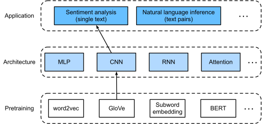
In this section, we will use the textCNN model to demonstrate how to design a CNN architecture for representing single text (Kim 2014). Compared with Figure 19.2.1 that uses an RNN architecture with GloVe pretraining for sentiment analysis, the only difference in Figure 19.3.1 lies in the choice of the architecture.
from d2l import tensorflow as d2l
import tensorflow as tf
import keras
import numpy as np

batch_size = 64
train_iter, test_iter, vocab = d2l.load_data_imdb(batch_size)
# d2l.load_array uses shuffle(buffer_size=1000), which is too small for
# the IMDb training set (25000 examples ordered as 12500 positives then
# 12500 negatives). Reshuffle the full dataset so each epoch sees a
# properly mixed class distribution, matching the PyTorch/JAX behavior.
train_iter = (train_iter.unbatch()
              .shuffle(25000, reshuffle_each_iteration=True)
              .batch(batch_size))
from d2l import jax as d2l
import jax
from jax import numpy as jnp
from flax import nnx
import optax
import numpy as np
batch_size = 256
train_iter, test_iter, vocab = d2l.load_data_imdb(batch_size)from d2l import mxnet as d2l
from mxnet import gluon, init, np, npx
from mxnet.gluon import nn
npx.set_np()
batch_size = 64
train_iter, test_iter, vocab = d2l.load_data_imdb(batch_size)19.3.1 One-Dimensional Convolutions
Before introducing the model, let’s see how a one-dimensional convolution works. Bear in mind that it is just a special case of a two-dimensional convolution based on the cross-correlation operation.

As shown in Figure 19.3.2, in the one-dimensional case, the convolution window slides from left to right across the input tensor. During sliding, the input subtensor (e.g., \(0\) and \(1\) in Figure 19.3.2) contained in the convolution window at a certain position and the kernel tensor (e.g., \(1\) and \(2\) in Figure 19.3.2) are multiplied elementwise. The sum of these multiplications gives the single scalar value (e.g., \(0\times1+1\times2=2\) in Figure 19.3.2) at the corresponding position of the output tensor.
We implement one-dimensional cross-correlation in the following corr1d function. Given an input tensor X and a kernel tensor K, it returns the output tensor Y.
def corr1d(X, K):
    w = K.shape[0]
    Y = d2l.zeros((X.shape[0] - w + 1))
    for i in range(Y.shape[0]):
        Y[i] = (X[i: i + w] * K).sum()
    return Y
def corr1d(X, K):
w = K.shape[0]
Y = [tf.reduce_sum(X[i: i + w] * K) for i in range(X.shape[0] - w + 1)]
return tf.stack(Y)def corr1d(X, K):
w = K.shape[0]
Y = d2l.zeros((X.shape[0] - w + 1))
for i in range(Y.shape[0]):
Y = Y.at[i].set((X[i: i + w] * K).sum())
return Ydef corr1d(X, K):
w = K.shape[0]
Y = d2l.zeros((X.shape[0] - w + 1))
for i in range(Y.shape[0]):
Y[i] = (X[i: i + w] * K).sum()
return YWe can construct the input tensor X and the kernel tensor K from Figure 19.3.2 to validate the output of the above one-dimensional cross-correlation implementation.
X, K = d2l.tensor([0, 1, 2, 3, 4, 5, 6]), d2l.tensor([1, 2])
corr1d(X, K)tensor([ 2., 5., 8., 11., 14., 17.])<tf.Tensor: shape=(6,), dtype=int32, numpy=array([ 2, 5, 8, 11, 14, 17], dtype=int32)>Array([ 2., 5., 8., 11., 14., 17.], dtype=float32)array([ 2., 5., 8., 11., 14., 17.])For any one-dimensional input with multiple channels, the convolution kernel needs to have the same number of input channels. Then for each channel, perform a cross-correlation operation on the one-dimensional tensor of the input and the one-dimensional tensor of the convolution kernel, summing the results over all the channels to produce the one-dimensional output tensor. Figure 19.3.3 shows a one-dimensional cross-correlation operation with 3 input channels.
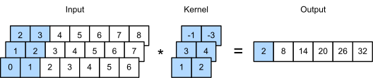
We can implement the one-dimensional cross-correlation operation for multiple input channels and validate the results in Figure 19.3.3.
def corr1d_multi_in(X, K):
    # First, iterate through the 0th dimension (channel dimension) of `X` and
    # `K`. Then, add them together
    return sum(corr1d(x, k) for x, k in zip(X, K))

X = d2l.tensor([[0, 1, 2, 3, 4, 5, 6],
              [1, 2, 3, 4, 5, 6, 7],
              [2, 3, 4, 5, 6, 7, 8]])
K = d2l.tensor([[1, 2], [3, 4], [-1, -3]])
corr1d_multi_in(X, K)tensor([ 2., 8., 14., 20., 26., 32.])<tf.Tensor: shape=(6,), dtype=int32, numpy=array([ 2, 8, 14, 20, 26, 32], dtype=int32)>Array([ 2., 8., 14., 20., 26., 32.], dtype=float32)array([ 2., 8., 14., 20., 26., 32.])Note that multi-input-channel one-dimensional cross-correlations are equivalent to single-input-channel two-dimensional cross-correlations. To illustrate, an equivalent form of the multi-input-channel one-dimensional cross-correlation in Figure 19.3.3 is the single-input-channel two-dimensional cross-correlation in Figure 19.3.4, where the height of the convolution kernel has to be the same as that of the input tensor.
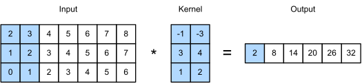
Both the outputs in Figure 19.3.2 and Figure 19.3.3 have only one channel. Same as two-dimensional convolutions with multiple output channels described in Section 6.4.2, we can also specify multiple output channels for one-dimensional convolutions.
19.3.2 Max-Over-Time Pooling
Similarly, we can use pooling to extract the highest value from sequence representations as the most important feature across time steps. The max-over-time pooling used in textCNN works like the one-dimensional global max-pooling (Collobert et al. 2011). For a multi-channel input where each channel stores values at different time steps, the output at each channel is the maximum value for that channel. Note that the max-over-time pooling allows different numbers of time steps at different channels.
19.3.3 The textCNN Model
Using the one-dimensional convolution and max-over-time pooling, the textCNN model takes individual pretrained token representations as input, then obtains and transforms sequence representations for the downstream application.
For a single text sequence with \(n\) tokens represented by \(d\)-dimensional vectors, the width, height, and number of channels of the input tensor are \(n\), \(1\), and \(d\), respectively. The textCNN model transforms the input into the output as follows:
- Define multiple one-dimensional convolution kernels and perform convolution operations separately on the inputs. Convolution kernels with different widths may capture local features among different numbers of adjacent tokens.
- Perform max-over-time pooling on all the output channels, and then concatenate all the scalar pooling outputs as a vector.
- Transform the concatenated vector into the output categories using the fully connected layer. Dropout can be used for reducing overfitting.
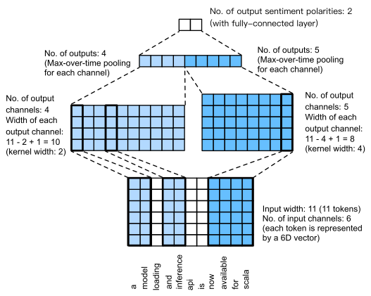
Figure 19.3.5 illustrates the model architecture of textCNN with a concrete example. The input is a sentence with 11 tokens, where each token is represented by a 6-dimensional vector. So we have a 6-channel input with width 11. Define two one-dimensional convolution kernels of widths 2 and 4, with 4 and 5 output channels, respectively. They produce 4 output channels with width \(11-2+1=10\) and 5 output channels with width \(11-4+1=8\). Despite different widths of these 9 channels, the max-over-time pooling gives a concatenated 9-dimensional vector, which is finally transformed into a 2-dimensional output vector for binary sentiment predictions.
19.3.3.1 Defining the Model
We implement the textCNN model in the following class. Compared with the bidirectional RNN model in Section 19.2, besides replacing recurrent layers with convolutional layers, we also use two embedding layers: one with trainable weights and the other with fixed weights.
class TextCNN(nn.Module):
    def __init__(self, vocab_size, embed_size, kernel_sizes, num_channels,
                 **kwargs):
        super(TextCNN, self).__init__(**kwargs)
        self.embedding = nn.Embedding(vocab_size, embed_size)
        # The embedding layer not to be trained
        self.constant_embedding = nn.Embedding(vocab_size, embed_size)
        self.dropout = nn.Dropout(0.5)
        self.decoder = nn.Linear(sum(num_channels), 2)
        # The max-over-time pooling layer has no parameters, so this instance
        # can be shared
        self.pool = nn.AdaptiveMaxPool1d(1)
        self.relu = nn.ReLU()
        # Create multiple one-dimensional convolutional layers
        self.convs = nn.ModuleList()
        for c, k in zip(num_channels, kernel_sizes):
            self.convs.append(nn.Conv1d(2 * embed_size, c, k))

    def forward(self, inputs):
        # Concatenate two embedding layer outputs with shape (batch size, no.
        # of tokens, token vector dimension) along vectors
        embeddings = torch.cat((
            self.embedding(inputs), self.constant_embedding(inputs)), dim=2)
        # Per the input format of one-dimensional convolutional layers,
        # rearrange the tensor so that the second dimension stores channels
        embeddings = embeddings.permute(0, 2, 1)
        # For each one-dimensional convolutional layer, after max-over-time
        # pooling, a tensor of shape (batch size, no. of channels, 1) is
        # obtained. Remove the last dimension and concatenate along channels
        encoding = torch.cat([
            torch.squeeze(self.relu(self.pool(conv(embeddings))), dim=-1)
            for conv in self.convs], dim=1)
        outputs = self.decoder(self.dropout(encoding))
        return outputs
class TextCNN(d2l.Classifier):
def __init__(self, vocab_size, embed_size, kernel_sizes, num_channels,
**kwargs):
super().__init__(**kwargs)
self.embedding = keras.layers.Embedding(vocab_size, embed_size)
# The embedding layer not to be trained
self.constant_embedding = keras.layers.Embedding(vocab_size, embed_size)
self.dropout = keras.layers.Dropout(0.5)
self.decoder = keras.layers.Dense(2)
# Create multiple one-dimensional convolutional layers
self.convs = [keras.layers.Conv1D(c, k, activation='relu')
for c, k in zip(num_channels, kernel_sizes)]
self.pool = keras.layers.GlobalMaxPooling1D()
def call(self, inputs, training=False):
# Concatenate two embedding layer outputs with shape
# (batch_size, num_steps, 2 * embed_size) along the last axis
embeddings = tf.concat(
[self.embedding(inputs), self.constant_embedding(inputs)], axis=2)
# For each convolutional layer, apply conv → global max pooling
# and collect a (batch_size, num_channels) vector per kernel
encoding = tf.concat(
[self.pool(conv(embeddings)) for conv in self.convs], axis=1)
outputs = self.decoder(self.dropout(encoding, training=training))
return outputsclass TextCNN(nnx.Module):
def __init__(self, vocab_size, embed_size, kernel_sizes, num_channels,
rngs=None):
rngs = nnx.Rngs(params=0, dropout=1) if rngs is None else rngs
self.embedding = nnx.Embed(vocab_size, embed_size, rngs=rngs)
# The embedding layer not to be trained
self.constant_embedding = nnx.Embed(vocab_size, embed_size, rngs=rngs)
self.dropout = nnx.Dropout(0.5, rngs=rngs)
self.decoder = nnx.Linear(sum(num_channels), 2, rngs=rngs)
# Create multiple one-dimensional convolutional layers
self.convs = nnx.List([
nnx.Conv(2 * embed_size, c, kernel_size=(k,), rngs=rngs)
for c, k in zip(num_channels, kernel_sizes)])
def __call__(self, inputs):
# Concatenate two embedding layer outputs with shape (batch size, no.
# of tokens, token vector dimension) along vectors
embeddings = jnp.concatenate((
self.embedding(inputs), self.constant_embedding(inputs)), axis=2)
# For Flax Conv, input shape is (batch, length, channels) which is
# already the shape of embeddings
# For each one-dimensional convolutional layer, after max-over-time
# pooling, a tensor of shape (batch size, no. of channels) is obtained.
# Concatenate along channels
encoding = jnp.concatenate([
jnp.max(nnx.relu(conv(embeddings)), axis=1)
for conv in self.convs], axis=1)
outputs = self.decoder(self.dropout(encoding))
return outputsclass TextCNN(nn.Block):
def __init__(self, vocab_size, embed_size, kernel_sizes, num_channels):
super().__init__()
self.embedding = nn.Embedding(vocab_size, embed_size)
# The embedding layer not to be trained
self.constant_embedding = nn.Embedding(vocab_size, embed_size)
self.dropout = nn.Dropout(0.5)
self.decoder = nn.Dense(2)
# The max-over-time pooling layer has no parameters, so this instance
# can be shared
self.pool = nn.GlobalMaxPool1D()
# Create multiple one-dimensional convolutional layers
self.convs = nn.Sequential()
for c, k in zip(num_channels, kernel_sizes):
self.convs.add(nn.Conv1D(c, k, activation='relu'))
def forward(self, inputs):
# Concatenate two embedding layer outputs with shape (batch size, no.
# of tokens, token vector dimension) along vectors
embeddings = np.concatenate((
self.embedding(inputs), self.constant_embedding(inputs)), axis=2)
# Per the input format of one-dimensional convolutional layers,
# rearrange the tensor so that the second dimension stores channels
embeddings = embeddings.transpose(0, 2, 1)
# For each one-dimensional convolutional layer, after max-over-time
# pooling, a tensor of shape (batch size, no. of channels, 1) is
# obtained. Remove the last dimension and concatenate along channels
encoding = np.concatenate([
np.squeeze(self.pool(conv(embeddings)), axis=-1)
for conv in self.convs], axis=1)
outputs = self.decoder(self.dropout(encoding))
return outputsLet’s create a textCNN instance. It has 3 convolutional layers with kernel widths of 3, 4, and 5, all with 100 output channels.
embed_size, kernel_sizes, nums_channels = 100, [3, 4, 5], [100, 100, 100]
devices = d2l.try_all_gpus()
net = TextCNN(len(vocab), embed_size, kernel_sizes, nums_channels)

def init_weights(module):
    if type(module) in (nn.Linear, nn.Conv1d):
        nn.init.xavier_uniform_(module.weight)

net.apply(init_weights);
embed_size, kernel_sizes, nums_channels = 100, [3, 4, 5], [100, 100, 100]
devices = d2l.try_all_gpus()
net = TextCNN(len(vocab), embed_size, kernel_sizes, nums_channels)
# Build the model by calling it once on a dummy input
dummy_input = tf.zeros((1, 500), dtype=tf.int32)
net(dummy_input)<tf.Tensor: shape=(1, 2), dtype=float32, numpy=array([[ 0.00163231, -0.02040011]], dtype=float32)>embed_size, kernel_sizes, nums_channels = 100, [3, 4, 5], [100, 100, 100]
devices = d2l.try_all_gpus()
net = TextCNN(len(vocab), embed_size, kernel_sizes, nums_channels)
d2l.check_shape(nnx.view(net, deterministic=True)(
jnp.ones((1, 500), dtype=jnp.int32)), (1, 2))embed_size, kernel_sizes, nums_channels = 100, [3, 4, 5], [100, 100, 100]
devices = d2l.try_all_gpus()
net = TextCNN(len(vocab), embed_size, kernel_sizes, nums_channels)
net.initialize(init.Xavier(), ctx=devices)19.3.3.2 Loading Pretrained Word Vectors
Same as Section 19.2, we load pretrained 100-dimensional GloVe embeddings as the initialized token representations. These token representations (embedding weights) will be trained in embedding and fixed in constant_embedding.
glove_embedding = d2l.TokenEmbedding('glove.6b.100d')
embeds = glove_embedding[vocab.idx_to_token]
net.embedding.weight.data.copy_(embeds)
net.constant_embedding.weight.data.copy_(embeds)
net.constant_embedding.weight.requires_grad = False
glove_embedding = d2l.TokenEmbedding('glove.6b.100d')
embeds = glove_embedding[vocab.idx_to_token]
net.embedding.set_weights([np.array(embeds)])
net.constant_embedding.set_weights([np.array(embeds)])
net.constant_embedding.trainable = Falseglove_embedding = d2l.TokenEmbedding('glove.6b.100d')
embeds = glove_embedding[vocab.idx_to_token]
# Set pretrained embedding weights in the parameters
net.embedding.embedding[...] = jnp.array(embeds)
net.constant_embedding.embedding = nnx.data(jnp.array(embeds))glove_embedding = d2l.TokenEmbedding('glove.6b.100d')
embeds = glove_embedding[vocab.idx_to_token]
net.embedding.weight.set_data(embeds)
net.constant_embedding.weight.set_data(embeds)
for p in net.constant_embedding.collect_params().values():
p.grad_req = 'null'19.3.3.3 Training and Evaluating the Model
Now we can train the textCNN model for sentiment analysis.
lr, num_epochs = 0.001, 5
trainer = torch.optim.Adam(net.parameters(), lr=lr)
loss = nn.CrossEntropyLoss(reduction="none")
d2l.train_ch13(net, train_iter, test_iter, loss, trainer, num_epochs, devices)
loss 0.093, train acc 0.969, test acc 0.865
13063.9 examples/sec on [device(type='cuda', index=0)]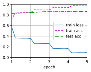
lr, num_epochs = 0.001, 5
net.compile(optimizer=keras.optimizers.Adam(lr),
            loss=keras.losses.SparseCategoricalCrossentropy(from_logits=True),
            metrics=['accuracy'])
net.fit(train_iter, validation_data=test_iter, epochs=num_epochs,
        verbose=2)
Epoch 1/5UserWarning: Your input ran out of data; interrupting training. Make sure that
your dataset or generator can generate at least `steps_per_epoch * epochs`
batches. You may need to use the `.repeat()` function when building your
dataset.391/391 - 24s - 60ms/step - accuracy: 0.7251 - loss: 0.5741 - val_accuracy: 0.8321 - val_loss: 0.3775
Epoch 2/5
391/391 - 3s - 9ms/step - accuracy: 0.8429 - loss: 0.3618 - val_accuracy: 0.8521 - val_loss: 0.3406
Epoch 3/5
391/391 - 3s - 8ms/step - accuracy: 0.8907 - loss: 0.2654 - val_accuracy: 0.8691 - val_loss: 0.3092
Epoch 4/5
391/391 - 3s - 9ms/step - accuracy: 0.9391 - loss: 0.1636 - val_accuracy: 0.8707 - val_loss: 0.3173
Epoch 5/5
391/391 - 3s - 9ms/step - accuracy: 0.9675 - loss: 0.0956 - val_accuracy: 0.8670 - val_loss: 0.3594<keras.src.callbacks.history.History at 0x74e570966b70>lr, num_epochs = 0.001, 5
optimizer = nnx.Optimizer(net, optax.adam(lr), wrt=nnx.Param)
loss_fn = optax.softmax_cross_entropy_with_integer_labels
@nnx.jit
def train_step(net, optimizer, X, y):
def compute_loss(model):
logits = model(X)
return loss_fn(logits, y).mean(), logits
(loss, logits), grads = nnx.value_and_grad(
compute_loss, has_aux=True)(net)
optimizer.update(net, grads)
return loss, logits
for epoch in range(num_epochs):
loss_sum, train_correct, num_train = (
jnp.array(0.0), jnp.array(0), 0)
for X, y in train_iter:
l, logits = train_step(net, optimizer, X, y)
loss_sum += l * len(y)
train_correct += (logits.argmax(axis=-1) == y).sum()
num_train += len(y)
# Evaluate
correct, total = jnp.array(0), 0
for X, y in test_iter:
logits = nnx.view(net, deterministic=True)(X)
correct += (logits.argmax(axis=-1) == y).sum()
total += len(y)
loss_sum, train_correct, correct = (
float(loss_sum), int(train_correct), int(correct))
print(f'epoch {epoch + 1}, loss {loss_sum / num_train:.3f}, '
f'train acc {train_correct / num_train:.3f}, '
f'test acc {correct / total:.3f}')epoch 1, loss 0.644, train acc 0.664, test acc 0.812
epoch 2, loss 0.413, train acc 0.811, test acc 0.842
epoch 3, loss 0.339, train acc 0.851, test acc 0.856
epoch 4, loss 0.280, train acc 0.886, test acc 0.866
epoch 5, loss 0.219, train acc 0.916, test acc 0.875lr, num_epochs = 0.001, 5
trainer = gluon.Trainer(net.collect_params(), 'adam', {'learning_rate': lr})
loss = gluon.loss.SoftmaxCrossEntropyLoss()
d2l.train_ch13(net, train_iter, test_iter, loss, trainer, num_epochs, devices)loss 0.094, train acc 0.967, test acc 0.865
1097.4 examples/sec on [gpu(0)]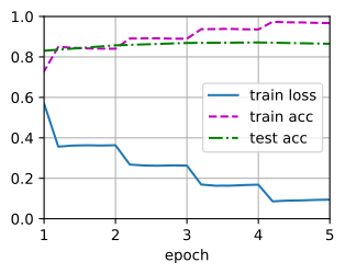
Below we use the trained model to predict the sentiment for two simple sentences.
d2l.predict_sentiment(net, vocab, 'this movie is so great')'positive'd2l.predict_sentiment(net, vocab, 'this movie is so great')'positive'tokens = jnp.array(vocab['this movie is so great'.split()])
logits = nnx.view(net, deterministic=True)(tokens.reshape(1, -1))
'positive' if int(jnp.argmax(logits, axis=1)[0]) == 1 else 'negative''positive'd2l.predict_sentiment(net, vocab, 'this movie is so great')'positive'd2l.predict_sentiment(net, vocab, 'this movie is so bad')'negative'd2l.predict_sentiment(net, vocab, 'this movie is so bad')'negative'tokens = jnp.array(vocab['this movie is so bad'.split()])
logits = nnx.view(net, deterministic=True)(tokens.reshape(1, -1))
'positive' if int(jnp.argmax(logits, axis=1)[0]) == 1 else 'negative''negative'd2l.predict_sentiment(net, vocab, 'this movie is so bad')'negative'19.3.4 Summary
- One-dimensional CNNs can process local features such as \(n\)-grams in text.
- Multi-input-channel one-dimensional cross-correlations are equivalent to single-input-channel two-dimensional cross-correlations.
- The max-over-time pooling allows different numbers of time steps at different channels.
- The textCNN model transforms individual token representations into downstream application outputs using one-dimensional convolutional layers and max-over-time pooling layers.
19.3.5 Exercises
- Tune hyperparameters and compare the two architectures for sentiment analysis in Section 19.2 and in this section, such as in classification accuracy and computational efficiency.
- Can you further improve the classification accuracy of the model by using the methods introduced in the exercises of Section 19.2?
- Add positional encoding in the input representations. Does it improve the classification accuracy?