%matplotlib inline
from d2l import torch as d2l
import torch
import numpy as onp4.1 Multilayer Perceptrons
Softmax regression maps its inputs to class scores with a single affine transformation. This makes the model easy to optimize but restricts its decision boundaries. Multilayer perceptrons add one or more hidden layers and nonlinear activation functions, allowing the model to represent nonlinear relations while retaining the same data, loss, and optimization procedure.
%matplotlib inline
from d2l import tensorflow as d2l
import tensorflow as tf
import numpy as onp%matplotlib inline
from d2l import jax as d2l
import jax
from jax import numpy as jnp
from jax import grad, vmap
import numpy as onp%matplotlib inline
from d2l import mxnet as d2l
from mxnet import autograd, np, npx
import numpy as onp
npx.set_np()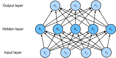
4.1.2 Activation Functions
Activation functions transform pre-activation signals into outputs and introduce nonlinearity into the network. Most are differentiable almost everywhere. We next examine several common choices.
4.1.2.1 ReLU Function
The most popular choice, due to both simplicity of implementation and its empirical performance across many predictive tasks, is the rectified linear unit (ReLU) (Nair and Hinton 2010). ReLU provides a very simple nonlinear transformation. Given an element \(x\), the function is defined as the maximum of that element and \(0\):
\[\operatorname{ReLU}(x) = \max(x, 0). \tag{4.1.2}\]
Informally, the ReLU function retains only positive elements and discards all negative elements by setting the corresponding activations to 0. To gain some intuition, we can plot the function. As you can see, the activation function is piecewise linear.
x = torch.arange(-8.0, 8.0, 0.1, requires_grad=True)
y = torch.relu(x)
d2l.plot(x.detach(), y.detach(), 'x', 'relu(x)', figsize=(5, 2.5))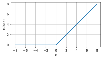
x = tf.Variable(tf.range(-8.0, 8.0, 0.1), dtype=tf.float32)
y = tf.nn.relu(x)
d2l.plot(x.numpy(), y.numpy(), 'x', 'relu(x)', figsize=(5, 2.5))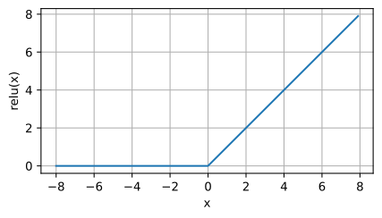
x = jnp.arange(-8.0, 8.0, 0.1)
y = jax.nn.relu(x)
d2l.plot(x, y, 'x', 'relu(x)', figsize=(5, 2.5))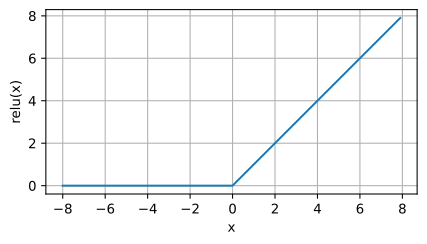
x = np.arange(-8.0, 8.0, 0.1)
x.attach_grad()
with autograd.record():
    y = npx.relu(x)
d2l.plot(x, y, 'x', 'relu(x)', figsize=(5, 2.5))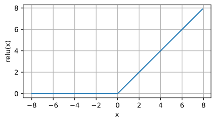
When the input is negative, the derivative of the ReLU function is 0, and when the input is positive, the derivative of the ReLU function is 1. Note that the ReLU function is not differentiable when the input takes value precisely equal to 0. The libraries used here return a derivative of 0 at the origin, one valid subgradient convention. For continuously distributed preactivations the choice affects a probability-zero event, but exact zeros do occur in computation, for example from zero-initialized biases or a preceding ReLU, and in such degenerate cases the convention can change whether a unit begins to move. We plot the derivative of the ReLU function below.
y.backward(torch.ones_like(x), retain_graph=True)
d2l.plot(x.detach(), x.grad, 'x', 'grad of relu', figsize=(5, 2.5))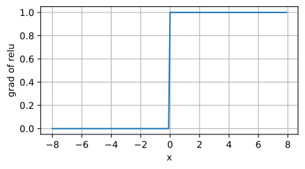
with tf.GradientTape() as t:
    y = tf.nn.relu(x)
d2l.plot(x.numpy(), t.gradient(y, x).numpy(), 'x', 'grad of relu',
         figsize=(5, 2.5))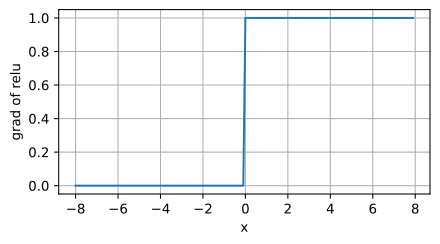
grad_relu = vmap(grad(jax.nn.relu))
d2l.plot(x, grad_relu(x), 'x', 'grad of relu', figsize=(5, 2.5))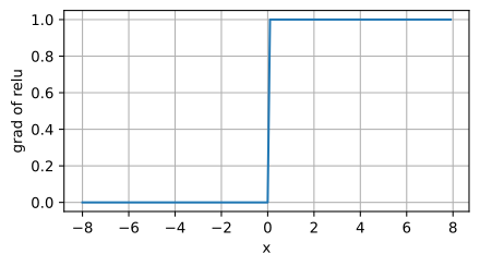
y.backward()
d2l.plot(x, x.grad, 'x', 'grad of relu', figsize=(5, 2.5))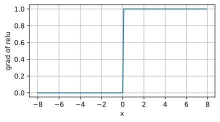
The reason for using ReLU is that its derivatives are particularly well behaved: they are either zero or one. This makes optimization better behaved and it mitigated the well-documented problem of vanishing gradients that plagued previous versions of neural networks (more on this later).
This same flatness has a downside, however. Because the gradient is exactly zero for negative inputs, a unit whose pre-activation is pushed negative for every training example receives no gradient and stops updating: it becomes a permanently silent dead ReLU. To keep gradient flowing in that regime, several variants retain a nonzero slope for negative inputs. A common example is the parametrized ReLU (pReLU) (He et al. 2015), which adds a linear term so some information still gets through, even when the argument is negative:
\[\operatorname{pReLU}(x) = \max(0, x) + \alpha \min(0, x). \tag{4.1.3}\]
Here \(\alpha\) is a small slope (fixed for leaky ReLU, learned for pReLU).
4.1.2.2 Sigmoid Function
The sigmoid function transforms those inputs whose values lie in the domain \(\mathbb{R}\), to outputs that lie on the interval (0, 1). For that reason, the sigmoid is often called a squashing function: it squashes any input in the range (-inf, inf) to some value in the range (0, 1):
\[\operatorname{sigmoid}(x) = \frac{1}{1 + \exp(-x)}. \tag{4.1.4}\]
In the earliest neural networks, scientists were interested in modeling biological neurons that either fire or do not fire. Thus the pioneers of this field, going all the way back to McCulloch and Pitts, the inventors of the artificial neuron, focused on thresholding units (McCulloch and Pitts 1943). A thresholding activation takes value 0 when its input is below some threshold and value 1 when the input exceeds the threshold.
When attention shifted to gradient-based learning, the sigmoid function was a natural choice because it is a smooth, differentiable approximation to a thresholding unit. Sigmoids are still widely used as activation functions on the output units when we want to interpret the outputs as probabilities for binary classification problems: you can think of the sigmoid as a special case of the softmax, namely the softmax over the two logits \(\{x, 0\}\). However, the sigmoid has largely been replaced by the simpler and more easily trainable ReLU for most use in hidden layers. Much of this has to do with the fact that the sigmoid poses challenges for optimization (LeCun et al. 1998) since its gradient vanishes for large positive and negative arguments. This can lead to plateaus that are difficult to escape from. Nonetheless sigmoids are important. In later chapters (e.g., Section 12.1) on recurrent neural networks, we will describe architectures that use sigmoid units to control the flow of information across time.
Below, we plot the sigmoid function. Note that when the input is close to 0, the sigmoid function approaches a linear transformation.
y = torch.sigmoid(x)
d2l.plot(x.detach(), y.detach(), 'x', 'sigmoid(x)', figsize=(5, 2.5))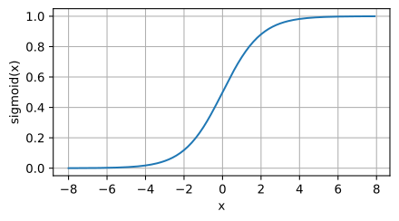
y = tf.nn.sigmoid(x)
d2l.plot(x.numpy(), y.numpy(), 'x', 'sigmoid(x)', figsize=(5, 2.5))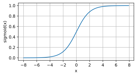
y = jax.nn.sigmoid(x)
d2l.plot(x, y, 'x', 'sigmoid(x)', figsize=(5, 2.5))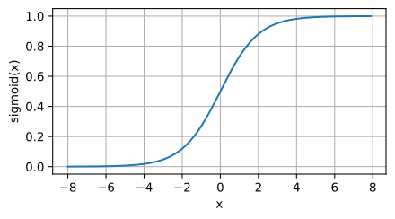
with autograd.record():
    y = npx.sigmoid(x)
d2l.plot(x, y, 'x', 'sigmoid(x)', figsize=(5, 2.5))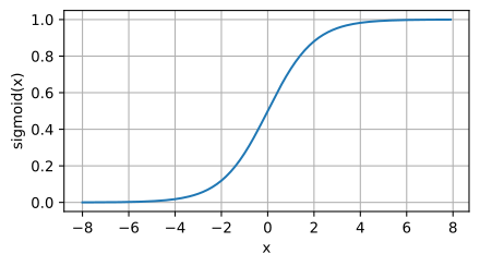
The derivative of the sigmoid function is given by the following equation:
\[\frac{d}{dx} \operatorname{sigmoid}(x) = \frac{\exp(-x)}{(1 + \exp(-x))^2} = \operatorname{sigmoid}(x)\left(1-\operatorname{sigmoid}(x)\right). \tag{4.1.5}\]
The derivative of the sigmoid function is plotted below. Note that when the input is 0, the derivative of the sigmoid function reaches a maximum of 0.25. As the input diverges from 0 in either direction, the derivative approaches 0.
# Clear out previous gradients
x.grad.zero_()
y.backward(torch.ones_like(x),retain_graph=True)
d2l.plot(x.detach(), x.grad, 'x', 'grad of sigmoid', figsize=(5, 2.5))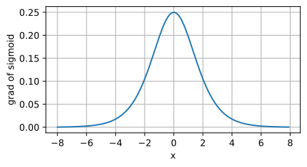
with tf.GradientTape() as t:
    y = tf.nn.sigmoid(x)
d2l.plot(x.numpy(), t.gradient(y, x).numpy(), 'x', 'grad of sigmoid',
         figsize=(5, 2.5))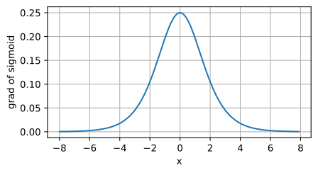
grad_sigmoid = vmap(grad(jax.nn.sigmoid))
d2l.plot(x, grad_sigmoid(x), 'x', 'grad of sigmoid', figsize=(5, 2.5))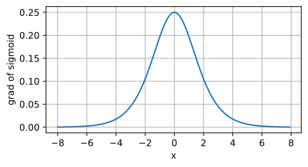
y.backward()
d2l.plot(x, x.grad, 'x', 'grad of sigmoid', figsize=(5, 2.5))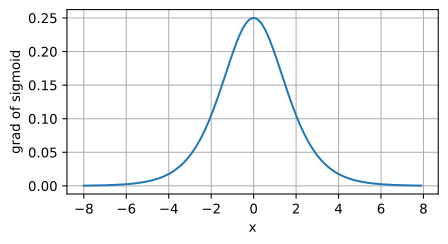
4.1.2.3 Tanh Function
Like the sigmoid function, the tanh (hyperbolic tangent) function also squashes its inputs, transforming them into elements on the interval between \(-1\) and \(1\):
\[\operatorname{tanh}(x) = \frac{1 - \exp(-2x)}{1 + \exp(-2x)}. \tag{4.1.6}\]
We plot the tanh function below. Note that as input nears 0, the tanh function approaches a linear transformation. Although the shape of the function is similar to that of the sigmoid function, the tanh function exhibits point symmetry about the origin of the coordinate system.
y = torch.tanh(x)
d2l.plot(x.detach(), y.detach(), 'x', 'tanh(x)', figsize=(5, 2.5))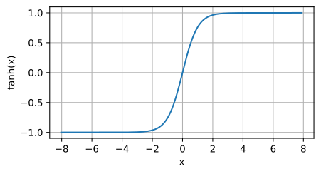
y = tf.nn.tanh(x)
d2l.plot(x.numpy(), y.numpy(), 'x', 'tanh(x)', figsize=(5, 2.5))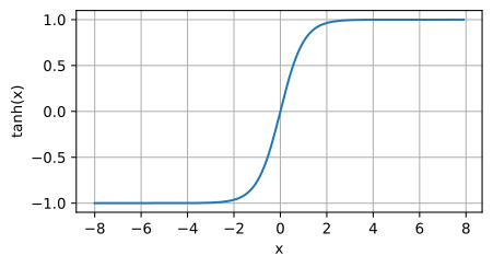
y = jax.nn.tanh(x)
d2l.plot(x, y, 'x', 'tanh(x)', figsize=(5, 2.5))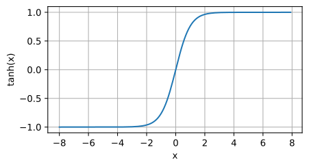
with autograd.record():
    y = np.tanh(x)
d2l.plot(x, y, 'x', 'tanh(x)', figsize=(5, 2.5))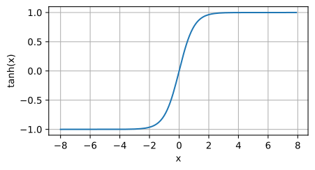
The derivative of the tanh function is:
\[\frac{d}{dx} \operatorname{tanh}(x) = 1 - \operatorname{tanh}^2(x). \tag{4.1.7}\]
It is plotted below. As the input nears 0, the derivative of the tanh function approaches a maximum of 1. And as we saw with the sigmoid function, as input moves away from 0 in either direction, the derivative of the tanh function approaches 0.
# Clear out previous gradients
x.grad.zero_()
y.backward(torch.ones_like(x),retain_graph=True)
d2l.plot(x.detach(), x.grad, 'x', 'grad of tanh', figsize=(5, 2.5))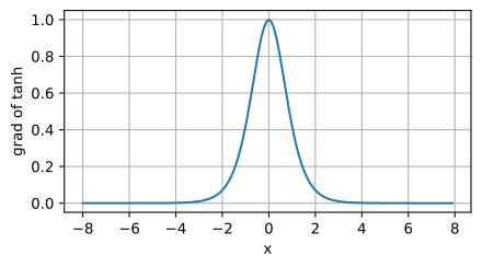
with tf.GradientTape() as t:
    y = tf.nn.tanh(x)
d2l.plot(x.numpy(), t.gradient(y, x).numpy(), 'x', 'grad of tanh',
         figsize=(5, 2.5))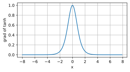
grad_tanh = vmap(grad(jax.nn.tanh))
d2l.plot(x, grad_tanh(x), 'x', 'grad of tanh', figsize=(5, 2.5))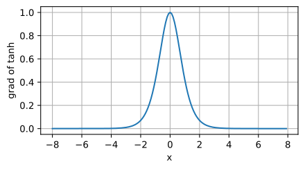
y.backward()
d2l.plot(x, x.grad, 'x', 'grad of tanh', figsize=(5, 2.5))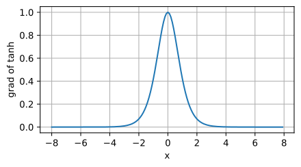
4.1.3 Summary and Discussion
Nonlinear activations prevent stacked affine layers from reducing to one affine map. They make MLPs expressive enough for nonlinear decision boundaries, while the universal approximation theorem supplies only a representational guarantee, not an optimization or generalization guarantee.
A key reason ReLU displaced sigmoid and tanh in hidden layers is that it is so much more amenable to optimization. One could argue that this was one of the innovations that helped the resurgence of deep learning in the early 2010s. Research on activation functions has not stopped, though, and you will meet newer ones once we reach the Transformer architectures later in the book. The most common are GELU (Gaussian error linear unit), \(x \Phi(x)\), where \(\Phi\) is the standard Gaussian cumulative distribution function (Hendrycks and Gimpel 2016), used in BERT and GPT-2-style models; Swish, \(x \operatorname{sigmoid}(\beta x)\) (Ramachandran et al. 2017); and SwiGLU (Shazeer 2020), a gated variant that is the default feedforward nonlinearity in recent large language models such as PaLM, LLaMA, and Mistral. For now, ReLU remains the sensible default for the models we build next.
4.1.4 Exercises
Linear networks. Stacking layers without a nonlinearity \(\sigma\) composes affine maps into another affine map, so depth never enlarges the function class of a linear network. Consider a linear network with input dimension \(d\), output dimension \(q\), and hidden widths \(h_1, \ldots, h_{L-1}\). Show that it represents exactly the affine maps \(\mathbf{X}\mathbf{W} + \mathbf{b}\) whose weight matrix \(\mathbf{W}\) has rank at most \(\min(h_1, \ldots, h_{L-1})\). Use this result to give an example in which adding a hidden layer to a linear model strictly shrinks its function class.
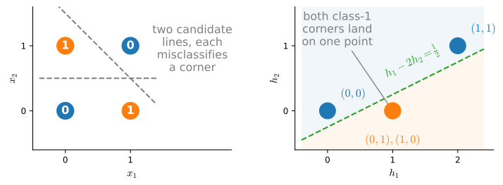
XOR by hand. Figure 4.1.2 gives one two-hidden-unit ReLU network that computes XOR by folding the two class-1 corners onto the same hidden point.
- Find a different set of weights for a two-hidden-unit ReLU network that also computes XOR but maps the two class-1 corners to distinct hidden points, and verify it on the four inputs.
- Show that no network with a single ReLU hidden unit and a linear output can compute XOR.
Activation derivatives. Compute the following derivatives.
- The derivatives of the pReLU activation function with respect to its input \(x\) and with respect to its slope \(\alpha\), for \(x \neq 0\).
- The derivative of the Swish activation function \(x \operatorname{sigmoid}(\beta x)\) with respect to \(x\). For fixed \(x \neq 0\), find its limits as \(\beta \to 0\) and as \(\beta \to \infty\), and identify the function that Swish approaches in each limit.
Piecewise linearity. Show that an MLP using only ReLU (or pReLU) constructs a continuous piecewise linear function.
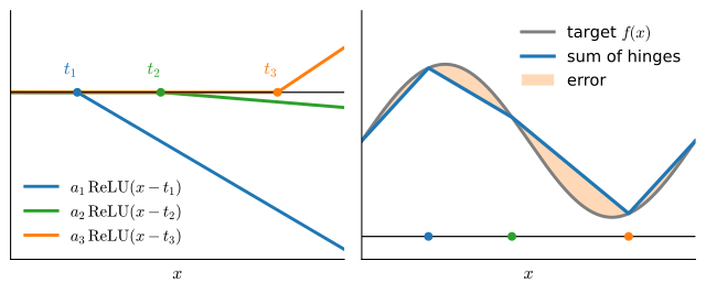
Depth and linear pieces. ● A one-hidden-layer ReLU network of width \(D\) on the real line has at most \(D + 1\) linear pieces (Figure 4.1.3), so width adds pieces only linearly. This problem makes the multiplicative effect of depth exact for one example.
- Take three hidden units \(\operatorname{ReLU}(w_k x + b_k)\) with input weights \(w_1 = w_2 = 1\) and \(w_3 = -1\) and with joints \(-b_k/w_k\) at \(1/6\), \(2/6\), and \(4/6\). Choose output weights and an output bias so that the network’s output \(g\) takes the values \(0, 1, 0, 1, 0\) at \(x = 0, 1/6, 2/6, 4/6, 1\).
- Count the linear pieces of \(g \circ g\) on \([0, 1]\) exactly, and of the \(K\)-fold composition \(g \circ \cdots \circ g\). Explain, in terms of how composing with \(g\) folds the graph, why each composition multiplies the count rather than adding to it.
- The \(K\)-fold composition is computed by a network with \(K\) hidden layers of three units each. How many hidden units would a single-hidden-layer network need to represent the same function? Compare the parameter counts of the two networks.
Adapted from Simon Prince, Understanding Deep Learning, Problem 4.8.
Sigmoid and tanh. Sigmoid and tanh are very similar.
- Show that \(\operatorname{tanh}(x) + 1 = 2 \operatorname{sigmoid}(2x)\).
- Show that for every MLP with tanh hidden activations there is an MLP of the same architecture with sigmoid hidden activations that computes the same function, and conversely. State how the weights and biases change.
Batch-wise nonlinearities. Consider a nonlinearity that acts jointly on a minibatch rather than on each example separately: for each hidden unit, it subtracts the minibatch mean and divides by the minibatch standard deviation. Batch normalization (Ioffe and Szegedy 2015) builds on this operation (Section 7.3). Suppose that prediction applies the same computation unchanged.
- Determine what the nonlinearity outputs for a batch of size \(1\).
- A test example is classified twice: once in a batch of examples drawn at random from the test set, and once in a batch whose other examples all belong to a single class. Compare the two predictions, and explain what the comparison implies for deploying the model.
[code] Vanishing gradients. Consider a chain of \(L\) sigmoid units of width one, \(h_l = \operatorname{sigmoid}(z_l)\) with pre-activation \(z_l = w_l h_{l-1} + b_l\). By the chain rule,
\[\frac{\partial h_L}{\partial h_0} = \prod_{l=1}^{L} w_l \operatorname{sigmoid}'(z_l). \tag{4.1.8}\]
- Explain why the weight feeding a saturated unit, one operating at large \(|z_l|\), receives almost no gradient whatever the loss, and why a single saturated unit also stalls every earlier layer of the chain.
- Choose the biases so that every pre-activation equals \(0\), where \(\operatorname{sigmoid}'\) attains its maximum \(1/4\). Compute the product for \(L = 1, \ldots, 20\), once with every \(w_l = 1\) and once with every \(w_l = 4\), and plot both curves on a logarithmic vertical axis.
- Repeat with every pre-activation equal to \(5\) and every \(w_l = 1\). Find the weight \(w\) for which \(w \operatorname{sigmoid}'(5) = 1\), and compare it with the weight that keeps the product constant at the origin. State what the comparison implies for training deep sigmoid networks in either regime.
[code] Weight scale and saturation. ● Take the chain of Exercise 8 with \(L = 20\), every weight \(w_l = w\), and every bias \(b_l = -w/2\), so that the input \(h_0 = 1/2\) gives \(z_l = 0\) at every layer.
- Express \(\partial h_L / \partial h_0\) as a function of \(w\) for the input \(h_0 = 1/2\). For which \(w\) does it not vanish as \(L\) grows?
- Implement the chain and run it from \(h_0 = 0.6\) with \(w = 4\) and with \(w = 8\). Report \(h_{20}\) and \(\partial h_{20} / \partial h_0\) in each case.
- Treat the map \(h_{l-1} \mapsto h_l\) as a one-dimensional iteration with fixed point \(1/2\), and use its slope there to explain the difference between the two runs. State what the result implies for countering vanishing gradients in a sigmoid network by scaling up its weights.
One hidden layer suffices. ● On the real line, Figure 4.1.3 approximates a continuous function with a single hidden layer, one hinge per joint. For two inputs, a natural extension uses two hidden layers: the first builds steps along the coordinate axes from pairs of ReLU units, and the second combines them into localized bumps, which are then summed. Show that the second hidden layer is unnecessary.
- Let \(\phi\) be continuous on \(\mathbb{R}\) and let \(\mathbf{w} \in \mathbb{R}^2\). Show that a single hidden layer approximates the ridge function \(\phi(\mathbf{w}^\top \mathbf{x})\), which is constant along every line orthogonal to \(\mathbf{w}\), uniformly on any compact subset of the plane.
- The Stone–Weierstrass theorem states the following. Let a set of continuous functions on a compact set be closed under sums, products, and scalar multiples, contain the constants, and contain, for any two distinct points, a function that takes different values at them. Then every continuous function on the compact set is a uniform limit of functions in the set. Show that the finite linear combinations of \(\cos(\boldsymbol{\omega}^\top \mathbf{x})\) and \(\sin(\boldsymbol{\omega}^\top \mathbf{x})\), with \(\boldsymbol{\omega} \in \mathbb{R}^2\), form such a set.
- Conclude that a single hidden layer approximates any continuous function on a compact subset of the plane.
Adapted from Michael Nielsen, Neural Networks and Deep Learning, Chapter 4.