%matplotlib inline
from d2l import torch as d2l
import torch
import numpy as onp  # plain NumPy for the probability demos
from scipy.special import digamma28.3 Mutual Information and Representation Learning
The entropies and divergences of Section 28.1 compare individual distributions. Mutual information instead measures the statistical dependence between two random variables. This quantity motivates several contrastive and self-supervised methods, including SimCLR, CPC, and CLIP-style dual encoders (Chen et al. 2020; Oord et al. 2018; Radford et al. 2021). Their InfoNCE objective provides a lower bound on mutual information. Such bounds are useful training objectives, but they are difficult to interpret as measurements: a distribution-free estimate based on \(N\) samples cannot in general certify much more than \(\log N\) nats. We first develop mutual information and the data-processing inequality, then study this estimation barrier, variational bounds, InfoNCE, and the information bottleneck.
As in Section 28.1, we work in nats (natural logarithm) throughout, flagging the occasional conversion to bits explicitly; recall \(1 \textrm{ bit} = \ln 2 \approx 0.693\) nats. We also lean on two facts from that section without re-proving them: Gibbs’ inequality (\(D_{\textrm{KL}} \geq 0\) with equality iff the distributions agree) and the decomposition \(\textrm{CE} = H + D_{\textrm{KL}}\).
Most of this section is plain-NumPy probability; the deep-learning library appears when we train a critic at the end of the variational-bounds section.
%matplotlib inline
from d2l import tensorflow as d2l
import tensorflow as tf
import numpy as onp  # plain NumPy for the probability demos
from scipy.special import digamma%matplotlib inline
from d2l import jax as d2l
import jax
from jax import numpy as jnp
import optax
import numpy as onp # plain NumPy for the probability demos
from scipy.special import digamma%matplotlib inline
from d2l import mxnet as d2l
from mxnet import autograd, gluon, init, np, npx
npx.set_np()
import numpy as onp # plain NumPy for the probability demos
from scipy.special import digamma28.3.1 Mutual Information: Definitions and Properties
Throughout, \((X,Y)\) is a pair of random variables with joint distribution \(P_{X,Y}\) and marginals \(P_X,P_Y\). We begin the entropy bookkeeping in the discrete case. For continuous variables the same symbols denote differential entropies only when the relevant integrals are finite; the KL definition of mutual information below remains primary and avoids undefined differences such as \(\infty-\infty\). The basic question is how observing \(Y\) changes our uncertainty about \(X\).
28.3.1.1 From One Variable to Two: Joint and Conditional Entropy
For discrete variables, the joint entropy averages the self-information of the pair:
\[H(X, Y) = -E_{(x, y) \sim P_{X,Y}} [\log p_{X, Y}(x, y)], \tag{28.3.1}\]
a sum over outcomes. The two extremes orient the discrete definition: if \(Y=X\), the pair carries no more information than either variable alone, \(H(X,Y)=H(X)\); if \(X\) and \(Y\) are independent, surprises add, \(H(X,Y)=H(X)+H(Y)\). Every discrete dependent pair sits between these bounds. For a continuous \(Y=X\), by contrast, the joint law lies on a lower-dimensional diagonal, has no ordinary joint density with respect to area, and has infinite mutual information; the discrete identity must not be transferred verbatim.
Often we care about a directed version of the question. Take \(X\) to be the pixels of an image and \(Y\) its class label. The image is a complicated, information-rich object, but once we have seen it, the label holds few surprises: a legible digit already reveals its class. The conditional entropy
\[H(Y \mid X) = - E_{(x, y) \sim P_{X,Y}} [\log p(y \mid x)], \tag{28.3.2}\]
with \(p(y \mid x) = p_{X,Y}(x, y)/p_X(x)\), measures exactly this residual: the average surprise in \(Y\) after \(X\) is known. The three quantities are linked by a bookkeeping identity.
Proposition (chain rule for entropy). For discrete variables, or for continuous variables when the displayed entropies are finite, \(H(X,Y)=H(X)+H(Y\mid X)\).
Proof. Inside the expectation defining \(H(X,Y)\), factor the joint density: \(\log p_{X,Y}(x,y) = \log p_X(x) + \log p(y \mid x)\). Taking \(-E_{(x,y) \sim P_{X,Y}}\) of both sides turns the left side into \(H(X,Y)\) and the two right-hand terms into \(H(X)\) and \(H(Y \mid X)\). \(\blacksquare\)
Read it as an accounting statement: the total information in the pair is the information in \(X\) plus whatever \(Y\) adds once \(X\) is known.
Consider the \(2 \times 2\) joint distribution
\[ p_{X,Y} = \begin{pmatrix} 0.1 & 0.4 \\ 0.2 & 0.3 \end{pmatrix}, \]
with rows indexing \(x \in \{0, 1\}\) and columns \(y \in \{0, 1\}\); the entries sum to \(1\) as a joint p.m.f. must. The marginals come from the joint by summing rows and columns: \(p_X = (0.5, 0.5)\) and \(p_Y = (0.3, 0.7)\). From the definitions, \(H(X,Y) \approx 1.2799\) nats, \(H(X) = \ln 2 \approx 0.6931\) nats, \(H(Y) \approx 0.6109\) nats, and the chain rule predicts \(H(Y \mid X) = H(X,Y) - H(X) \approx 0.5867\) nats, which the direct definition Equation 28.3.2 confirms.
p_xy = onp.array([[0.1, 0.4],
                  [0.2, 0.3]])           # a valid joint: entries sum to 1
p_x, p_y = p_xy.sum(axis=1), p_xy.sum(axis=0)  # marginals FROM the joint

entropy = lambda p: float(-(p * onp.log(p)).sum())
H_xy, H_x, H_y = entropy(p_xy), entropy(p_x), entropy(p_y)
# Conditional entropy directly: p(y|x) = p(x,y) / p(x), weighted by p(x,y)
H_y_given_x = float(-(p_xy * onp.log(p_xy / p_x[:, None])).sum())

print(f'marginals: p_x = {p_x}, p_y = {p_y}')
print(f'H(X,Y) = {H_xy:.4f}, H(X) = {H_x:.4f}, H(Y) = {H_y:.4f} nats')
print(f'H(Y|X) = {H_y_given_x:.4f} = H(X,Y) - H(X) = {H_xy - H_x:.4f} nats')
marginals: p_x = [0.5 0.5], p_y = [0.3 0.7]
H(X,Y) = 1.2799, H(X) = 0.6931, H(Y) = 0.6109 nats
H(Y|X) = 0.5867 = H(X,Y) - H(X) = 0.5867 nats28.3.1.2 Mutual Information as a Divergence from Independence
The conditional entropy measured what \(Y\) keeps to itself; we want what \(X\) and \(Y\) share. The definition needs no entropy at all. If \(X\) and \(Y\) were independent, their joint distribution would be the product of marginals \(P_X \otimes P_Y\), with density \(p_X(x)\,p_Y(y)\). The mutual information is the KL divergence from that hypothetical independent world to the actual joint:
\[I(X; Y) = D_{\textrm{KL}}\!\left(P_{X,Y} \,\|\, P_X \otimes P_Y\right) = E_{(x, y) \sim P_{X,Y}} \left[ \log\frac{p_{X, Y}(x, y)}{p_X(x)\, p_Y(y)} \right]. \tag{28.3.3}\]
In words: mutual information is how far the pair is from being independent, measured in the same units as every other quantity in this chapter. (The semicolon in \(I(X; Y)\) is the standard notation, distinguishing the two arguments from a single joint object.) The definition presumes the joint has a density with respect to the product of the marginals; when it does not, for instance when \(Y = f(X)\) is a deterministic function of a continuous \(X\), the divergence is infinite, and so is \(I(X; Y)\). Symmetry and nonnegativity are immediate from the divergence form, and the entropy identities follow by expanding the logarithm.
Proposition (properties of mutual information). For any pair \((X,Y)\), \(I(X;Y)\) is symmetric and non-negative, with equality if and only if \(X\) and \(Y\) are independent. When the relevant discrete or differential entropies are finite, it also satisfies
\[ I(X;Y)=H(X)+H(Y)-H(X,Y)=H(X)-H(X\mid Y)=H(Y)-H(Y\mid X). \]
Proof. When the entropy terms are finite, expand the logarithm in Equation 28.3.3:
\[ \begin{aligned} I(X; Y) &= E\left[\log p_{X,Y}(x,y)\right] - E\left[\log p_X(x)\right] - E\left[\log p_Y(y)\right] \\ &= -H(X,Y) + H(X) + H(Y). \end{aligned} \]
Substituting the chain rule \(H(X,Y) = H(Y) + H(X \mid Y)\) gives \(I(X;Y) = H(X) - H(X \mid Y)\), and the symmetric substitution gives \(H(Y) - H(Y \mid X)\). Symmetry is immediate from Equation 28.3.3, whose density ratio is unchanged when \(X\) and \(Y\) are swapped. Nonnegativity is Gibbs’ inequality (Section 28.1) applied to the two distributions \(P_{X,Y}\) and \(P_X \otimes P_Y\): the divergence is non-negative, and zero exactly when they coincide, i.e., when \(p_{X,Y}(x,y) = p_X(x)\,p_Y(y)\) everywhere, which is the definition of independence. \(\blacksquare\)
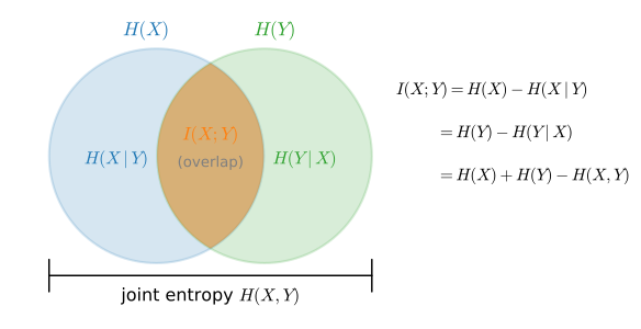
The identities have a picture, Figure 28.3.1: draw \(H(X)\) and \(H(Y)\) as overlapping disks. The overlap is \(I(X;Y)\), the crescents are the conditional entropies, the union is the joint entropy, and each identity in claim 1 is one way of reading off the overlap’s area. The picture also explains the directed reading: \(I(X;Y) = H(X) - H(X \mid Y)\) is the reduction in surprise about \(X\) obtained by observing \(Y\).
Back to the worked example. With marginals computed from the joint, the divergence form Equation 28.3.3 and the entropy identity must return the same number, and they do: \(I(X;Y) \approx 0.0242\) nats (\(\approx 0.035\) bits after dividing by \(\ln 2\)). The pair is barely dependent: the joint \(\begin{smallmatrix}0.1 & 0.4\\0.2 & 0.3\end{smallmatrix}\) is close to the product of its marginals \(\begin{smallmatrix}0.15 & 0.35\\0.15 & 0.35\end{smallmatrix}\), and mutual information quantifies the gap.
def mutual_information(p_xy):
    """I(X;Y) of a discrete joint p.m.f., in nats."""
    p_x = p_xy.sum(axis=1, keepdims=True)   # marginals from the joint
    p_y = p_xy.sum(axis=0, keepdims=True)
    return float((p_xy * onp.log(p_xy / (p_x * p_y))).sum())

mi_kl = mutual_information(p_xy)            # divergence form
mi_ent = H_x + H_y - H_xy                    # entropy identity
print(f'I(X;Y) = {mi_kl:.4f} nats (KL form) '
      f'= {mi_ent:.4f} nats (entropy identity)')
print(f'       = {mi_kl / onp.log(2):.4f} bits')
I(X;Y) = 0.0242 nats (KL form) = 0.0242 nats (entropy identity)
= 0.0349 bits28.3.1.3 A Gaussian Example
For continuous variables, the bivariate Gaussian provides a useful worked example with a closed form. We use this expression as a known reference value for the estimators below.
Proposition (Gaussian mutual information). If \((X, Y)\) is bivariate Gaussian with correlation coefficient \(\rho\), then
\[I(X; Y) = -\tfrac{1}{2} \log\left(1 - \rho^2\right). \tag{28.3.4}\]
Proof. Mutual information is invariant under separate invertible maps of \(X\) and of \(Y\) (proved in the next subsection), so we may standardize both variables and take
\[ \Sigma = \begin{pmatrix} 1 & \rho \\ \rho & 1 \end{pmatrix}, \qquad \det \Sigma = 1 - \rho^2. \]
For a standard Gaussian the differential entropy is \(h(X) = h(Y) = \tfrac{1}{2}\log(2\pi e)\), a value computed explicitly inside the maximum-entropy proof of Section 28.1.2.3; the same integration against the bivariate density gives \(h(X, Y) = \tfrac{1}{2}\log\left((2\pi e)^2 \det\Sigma\right)\). The entropy identity of claim 1 carries over: joint and conditional differential entropies are the same formulas with integrals in place of sums, and the chain-rule algebra never used discreteness. It gives
\[ I(X; Y) = h(X) + h(Y) - h(X, Y) = \log(2\pi e) - \tfrac{1}{2}\log\left((2\pi e)^2 (1 - \rho^2)\right) = -\tfrac{1}{2}\log(1 - \rho^2). \]
Each differential entropy individually depends on the coordinates (recall the caveat of Section 28.1: differential entropy can even be negative), but the offending terms cancel in the combination: mutual information is a relative quantity. \(\blacksquare\)
Read the limits: at \(\rho = 0\) the variables are independent (for Gaussians, uncorrelated implies independent) and \(I = 0\); as \(\rho \to \pm 1\) the joint density collapses onto a line, \(Y\) determines \(X\), and \(I \to \infty\). In between, the formula gives concrete targets: \(\rho = 0.5\) carries \(\approx 0.144\) nats, \(\rho = 0.9\) carries \(\approx 0.830\) nats, and \(\rho = 0.99\) carries \(\approx 1.96\) nats.
The following example estimates Equation 28.3.4 by binning the samples into a 2-D histogram and applying the discrete formula to the bin frequencies.
def gauss_pair(rng, rho, n):
    """n samples of a standard bivariate Gaussian with correlation rho."""
    x = rng.standard_normal(n)
    y = rho * x + onp.sqrt(1 - rho**2) * rng.standard_normal(n)
    return x, y

def binned_mi(x, y, bins=40):
    """Plug-in MI estimate from a 2-D histogram, in nats."""
    counts, _, _ = onp.histogram2d(x, y, bins=bins)
    p = counts / counts.sum()
    p_x, p_y = p.sum(axis=1, keepdims=True), p.sum(axis=0, keepdims=True)
    mask = p > 0
    return float((p[mask] * onp.log(p[mask] / (p_x * p_y)[mask])).sum())

rng = onp.random.default_rng(42)
rhos = onp.array([0.0, 0.3, 0.6, 0.9, 0.99])
est = [binned_mi(*gauss_pair(rng, r, 200_000)) for r in rhos]
true = [-0.5 * onp.log(1 - r**2) for r in rhos]
for r, e, t in zip(rhos, est, true):
    print(f'rho = {r:4.2f}: binned = {e:.4f}, closed form = {t:.4f} nats')
d2l.plot(rhos, [onp.array(est), onp.array(true)], 'correlation rho',
         'I(X;Y) (nats)', legend=['binned estimate', 'closed form'],
figsize=(5, 3))rho = 0.00: binned = 0.0027, closed form = -0.0000 nats
rho = 0.30: binned = 0.0504, closed form = 0.0472 nats
rho = 0.60: binned = 0.2235, closed form = 0.2231 nats
rho = 0.90: binned = 0.8111, closed form = 0.8304 nats
rho = 0.99: binned = 1.7829, closed form = 1.9585 nats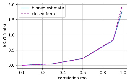
rho = 0.00: binned = 0.0027, closed form = -0.0000 nats
rho = 0.30: binned = 0.0504, closed form = 0.0472 nats
rho = 0.60: binned = 0.2235, closed form = 0.2231 nats
rho = 0.90: binned = 0.8111, closed form = 0.8304 nats
rho = 0.99: binned = 1.7829, closed form = 1.9585 nats
rho = 0.00: binned = 0.0027, closed form = -0.0000 nats
rho = 0.30: binned = 0.0504, closed form = 0.0472 nats
rho = 0.60: binned = 0.2235, closed form = 0.2231 nats
rho = 0.90: binned = 0.8111, closed form = 0.8304 nats
rho = 0.99: binned = 1.7829, closed form = 1.9585 nats
rho = 0.00: binned = 0.0027, closed form = -0.0000 nats
rho = 0.30: binned = 0.0504, closed form = 0.0472 nats
rho = 0.60: binned = 0.2235, closed form = 0.2231 nats
rho = 0.90: binned = 0.8111, closed form = 0.8304 nats
rho = 0.99: binned = 1.7829, closed form = 1.9585 nats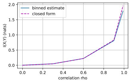
With \(200{,}000\) samples and a \(40 \times 40\) grid, the histogram tracks the closed form well at moderate correlation, but look closely at \(\rho = 0.99\): the estimate comes in at roughly \(1.78\) nats against a truth of \(1.96\), missing about \(0.18\) nats because the probability mass hides in a ridge thinner than the bins. Even in two dimensions with abundant data, the plug-in histogram estimator is already biased once the dependence is strong. The high-dimensional estimators developed below face still sharper limits.
28.3.1.4 Pointwise Mutual Information
Mutual information is an average. Its summand in Equation 28.3.3 is the pointwise mutual information
\[\textrm{pmi}(x, y) = \log\frac{p_{X, Y}(x, y)}{p_X(x)\, p_Y(y)} \tag{28.3.5}\]
compares how often the specific pair \((x, y)\) occurs to how often it would occur if \(X\) and \(Y\) were independent. Positive pmi means the outcomes attract (they co-occur more than chance predicts); negative pmi means they repel; and \(I(X;Y) = E[\textrm{pmi}(x,y)]\) is the average attraction.
Pointwise mutual information is widely used in natural language processing (Church and Hanks 1990), where it separates genuine collocations from words that merely co-occur because both are common. Here is the effect in miniature. Suppose we count consecutive word pairs (bigrams) in a small corpus and tally how often each of the first words new, machine, the is followed by each of york, learning, day:
| count | york | learning | day |
|---|---|---|---|
| new | 38 | 3 | 9 |
| machine | 1 | 46 | 3 |
| the | 11 | 21 | 168 |
The raw counts mislead: “the day” is by far the most frequent pair (\(168\) occurrences against \(38\) for “new york”), because the and day are both frequent words. Pointwise mutual information corrects for the marginals.
counts = onp.array([[38., 3., 9.],     # new york / new learning / new day
                    [1., 46., 3.],     # machine ...
                    [11., 21., 168.]]) # the ...
first, second = ['new', 'machine', 'the'], ['york', 'learning', 'day']

p = counts / counts.sum()
p_w, p_c = p.sum(axis=1, keepdims=True), p.sum(axis=0, keepdims=True)
pmi = onp.log(p / (p_w * p_c))
for (i, j) in [(0, 0), (1, 1), (2, 2), (2, 0)]:
    print(f'pmi({first[i]}, {second[j]}) = {pmi[i, j]:6.3f} nats '
          f'(count {counts[i, j]:.0f})')
print(f'I(first; second) = {float((p * pmi).sum()):.4f} nats')
pmi(new, york) = 1.517 nats (count 38)
pmi(machine, learning) = 1.372 nats (count 46)
pmi(the, day) = 0.336 nats (count 168)
pmi(the, york) = -1.109 nats (count 11)
I(first; second) = 0.4146 natsAfter adjustment for the marginals, the collocations receive the higher scores: “new york” scores \(\textrm{pmi} \approx 1.52\) nats and “machine learning” \(\approx 1.37\), while the frequent-but-unremarkable “the day” manages only \(\approx 0.34\); the pair “the york” comes out negative (\(\approx -1.11\) nats), occurring three times less often than independence would predict. The table’s overall mutual information is \(\approx 0.41\) nats, summarizing how strongly first words constrain second words on average. This count-divide-and-log pattern (and its smoothed variants) underpins classical word-association mining and survives inside modern embedding methods, where factorizing a pmi matrix recovers word vectors (Levy and Goldberg 2014).
28.3.1.5 Mutual Information as Nonlinear Correlation
How does mutual information relate to the correlation coefficient of Section 27.1? Correlation detects linear dependence: \(\rho(X, Y) = 0\) does not imply independence, only the absence of a linear trend. Mutual information detects any dependence: by claim 3 of the properties proposition, \(I(X; Y) = 0\) holds if and only if \(X \perp Y\). Two further properties sharpen the contrast.
Proposition (reparameterization invariance). If \(g\) and \(h\) are invertible maps (in the continuous case, smooth with smooth inverses), then \(I(g(X); h(Y)) = I(X; Y)\).
Proof. For discrete variables, invertibility means \(g\) and \(h\) merely relabel outcomes: the joint p.m.f. of \((g(X), h(Y))\) takes the same values as that of \((X, Y)\) at different labels, and the sum in Equation 28.3.3 is unchanged. For continuous variables, write mutual information as the KL divergence \(D_{\textrm{KL}}(P_{X,Y} \| P_X \otimes P_Y)\) and apply the smooth change of variables \((x, y) \mapsto (g(x), h(y))\): both densities in the ratio pick up the same Jacobian factor \(|g'(x)|^{-1} |h'(y)|^{-1}\), which cancels. (Contrast differential entropy, where the uncancelled Jacobian is exactly why it is coordinate-dependent; see Section 28.1.) \(\blacksquare\)
Correlation enjoys no such invariance: it is preserved only by affine maps (up to sign). Mutual information therefore captures a broader notion of dependence: it asks whether two variables are informative about each other in any coordinates, not only whether they align linearly. A standard counterexample makes both points at once: let \(X \sim \mathcal{N}(0, 1)\) and \(Y = X^2 + 0.3\,\epsilon\) with independent noise \(\epsilon \sim \mathcal{N}(0,1)\). Then \(\textrm{Cov}(X, Y) = E[X^3] = 0\) by symmetry, so the correlation vanishes, yet \(Y\) is nearly a function of \(X\), and the dependence is strong.
rng = onp.random.default_rng(0)
n = 200_000
x = rng.standard_normal(n)
y = x**2 + 0.3 * rng.standard_normal(n)    # zero correlation by symmetry

print(f'sample correlation rho = {onp.corrcoef(x, y)[0, 1]:+.4f}')
print(f'binned MI estimate     = {binned_mi(x, y):.4f} nats')
print(f'after x -> 2x + 3      = {binned_mi(2 * x + 3, y):.4f} nats')
sample correlation rho = -0.0028
binned MI estimate = 0.9814 nats
after x -> 2x + 3 = 0.9814 natsThe correlation is numerically zero while the mutual information estimate is about one nat, more shared information than the \(\rho = 0.9\) Gaussian pair above (\(0.830\) nats). The third line checks invariance: an affine reparameterization of \(X\) leaves the estimate exactly unchanged (the histogram bins stretch with the data, so even the bin counts are identical). One caution for later: this invariance is also why mutual information is hard to estimate, since an estimator must implicitly cope with every reparameterization of the data at once; Section 28.3.2 describes the resulting estimation cost.
28.3.1.6 Conditional Mutual Information and the Chain Rule
Like entropy, mutual information has a conditional version. The conditional mutual information
\[I(X; Y \mid Z) = H(X \mid Z) - H(X \mid Y, Z) \tag{28.3.6}\]
is the information \(X\) and \(Y\) share once \(Z\) is already known. Equivalently, \(I(X; Y \mid Z) = E_{z}\left[D_{\textrm{KL}}(P_{X,Y \mid z} \,\|\, P_{X \mid z} \otimes P_{Y \mid z})\right]\): expanding each conditional entropy as an expectation and collecting the logarithms into the ratio \(p_{X,Y \mid z}/(p_{X \mid z}\, p_{Y \mid z})\) repeats the algebra of claim 1 under each conditional law. As an average of per-\(z\) divergences it inherits nonnegativity from Gibbs, with \(I(X; Y \mid Z) = 0\) if and only if \(X\) and \(Y\) are conditionally independent given \(Z\). The chain rule then splits joint information into sequential contributions.
Proposition (chain rule for mutual information). For any \(X, Y, Z\),
\[ I(X; Y, Z) = I(X; Z) + I(X; Y \mid Z). \]
Proof. Telescope with the entropy identities:
\[ \begin{aligned} I(X; Y, Z) &= H(X) - H(X \mid Y, Z) \\ &= \underbrace{H(X) - H(X \mid Z)}_{I(X;\, Z)} + \underbrace{H(X \mid Z) - H(X \mid Y, Z)}_{I(X;\, Y \mid Z)}. \quad\blacksquare \end{aligned} \]
Corollary (independent side information is free). If \(W\) is independent of the pair \((X, Y)\), then \(I(X; (Y, W)) = I(X; Y)\).
Proof. By the chain rule, \(I(X; Y, W) = I(X; W) + I(X; Y \mid W)\). The first term is zero since \(W \perp X\). For the second, independence of \(W\) from the pair means conditioning on \(W\) changes neither \(H(X)\) nor \(H(X \mid Y)\), so \(I(X; Y \mid W) = I(X; Y)\). \(\blacksquare\)
The corollary is exactly the accounting we will need for InfoNCE in Section 28.3.3.4, where a batch of independent “negative” samples is appended to \(Y\) and must add no information about \(X\). The chain rule’s main consequence deserves its own subsection.
28.3.1.7 The Data-Processing Inequality
Random variables \(X, Y, Z\) form a Markov chain, written \(X \to Y \to Z\), when \(Z\) depends on \((X, Y)\) only through \(Y\): \(p(z \mid x, y) = p(z \mid y)\). This is the structure of processing: \(Y\) is computed from \(X\) (a measurement, a feature map, a hidden layer), then \(Z\) is computed from \(Y\) alone. Equivalently, \(X\) and \(Z\) are conditionally independent given \(Y\), i.e., \(I(X; Z \mid Y) = 0\). The following theorem (Cover and Thomas 1999) governs this structure.
Proposition (data-processing inequality). If \(X \to Y \to Z\) is a Markov chain, then
\[ I(X; Z) \leq I(X; Y), \]
with equality if and only if \(I(X; Y \mid Z) = 0\) (i.e., \(X \to Z \to Y\) is also a Markov chain).
Proof. Expand \(I(X; Y, Z)\) by the chain rule in both orders:
\[ I(X; Z) + I(X; Y \mid Z) = I(X; Y, Z) = I(X; Y) + I(X; Z \mid Y). \]
The Markov property makes the last term zero, \(I(X; Z \mid Y) = 0\), leaving \(I(X; Z) = I(X; Y) - I(X; Y \mid Z) \leq I(X; Y)\), since conditional mutual information is non-negative. Equality holds exactly when \(I(X; Y \mid Z) = 0\). \(\blacksquare\)
No deterministic or random processing of \(Y\) can increase the information it carries about \(X\). Three consequences follow:
- Representations only lose. A network computes its representation layer-by-layer, \(X \to Z_1 \to Z_2 \to \cdots\), so \(I(X; Z_1) \geq I(X; Z_2) \geq \cdots\) and likewise \(I(Y; Z_1) \geq I(Y; Z_2) \geq \cdots\) for a label \(Y\) at the input end of the chain (since \(Y \to X \to Z_\ell\) is Markov). Whatever label information the input lacks, no architecture can create; whatever a layer discards, no later layer recovers. This is the theorem that makes the information bottleneck of Section 28.3.4 a well-defined objective.
- Equality is achievable. If \(Z = g(Y)\) for an invertible \(g\), then the chain runs both ways and \(I(X; Z) = I(X; Y)\), consistent with the reparameterization invariance proved earlier. A many-to-one or noisy map may lose information, but it need not: a sufficient statistic can be noninvertible or noisy while preserving all the information about \(X\). Equality in data processing is characterized by such sufficiency, not by invertibility alone.
- A sufficient statistic is a lossless compression. When equality holds with \(Z\) much “smaller” than \(Y\), the map has discarded only what was irrelevant to \(X\): this is the information-theoretic reading of a sufficient statistic (Section 27.2).
One caution about scope. The data-processing inequality is a statement about Markov chains, not about conditioning in general. Conditioning can create dependence, and \(I(X; Y \mid Z) > I(X; Y)\) is perfectly possible: in the extreme case of two independent fair bits with \(Z\) their XOR, conditioning turns zero dependence into a full \(\ln 2\) nats (Exercise 6 works this out). “Processing destroys information” is a theorem about the chain \(X \to Y \to Z\) alone; outside that structure, conditioning can raise or lower dependence, as the XOR example shows.
The following example verifies the bookkeeping on a simple nontrivial chain: a fair bit \(X\), flipped with probability \(0.1\) to give \(Y\), flipped again with probability \(0.2\) to give \(Z\).
p_x = onp.array([0.5, 0.5])
K1 = onp.array([[0.9, 0.1], [0.1, 0.9]])   # p(y|x): flip w.p. 0.1
K2 = onp.array([[0.8, 0.2], [0.2, 0.8]])   # p(z|y): flip w.p. 0.2
p_xyz = p_x[:, None, None] * K1[:, :, None] * K2[None, :, :]

def cond_mi(p_abc):
    """I(A;B|C) for a joint array indexed [a, b, c], in nats."""
    p_ac, p_bc, p_c = p_abc.sum(1), p_abc.sum(0), p_abc.sum((0, 1))
    ratio = p_abc * p_c[None, None, :] / (p_ac[:, None, :] * p_bc[None, :, :])
    return float((p_abc * onp.log(ratio)).sum())

I_xy = mutual_information(p_xyz.sum(axis=2))           # I(X;Y)
I_xz = mutual_information(p_xyz.sum(axis=1))           # I(X;Z)
I_xz_y = cond_mi(onp.transpose(p_xyz, (0, 2, 1)))      # I(X;Z|Y)
I_xy_z = cond_mi(p_xyz)                                # I(X;Y|Z)
print(f'I(X;Y) = {I_xy:.4f},  I(X;Z) = {I_xz:.4f} nats  (DPI: smaller)')
print(f'I(X;Z|Y) = {I_xz_y:.4f}  (Markov: zero)')
print(f'chain rule, both orders: {I_xz + I_xy_z:.4f} = {I_xy + I_xz_y:.4f}')
I(X;Y) = 0.3681, I(X;Z) = 0.1201 nats (DPI: smaller)
I(X;Z|Y) = 0.0000 (Markov: zero)
chain rule, both orders: 0.3681 = 0.3681Every claim checks out: \(I(X; Z \mid Y) = 0\) certifies the Markov structure, both expansions of \(I(X; Y, Z)\) agree at \(0.3681\) nats, and processing through the second noisy channel costs two thirds of the information: \(I(X;Y) \approx 0.368\) nats falls to \(I(X;Z) \approx 0.120\) nats. (For calibration, a noiseless bit would carry \(\ln 2 \approx 0.693\) nats.)
28.3.2 Why Measuring Mutual Information Is Hard
The next problem is to estimate mutual information from samples, such as images and their augmentations or sentences and their continuations. This is substantially harder than evaluating the closed-form examples above.
28.3.2.1 Estimation in High Dimensions
The histogram plug-in estimator used above scales poorly in high dimensions. With \(b\) bins per axis, a \(d\)-dimensional histogram has \(b^d\) cells; at \(d = 10\) and a modest \(b = 10\) that is ten billion cells, almost all empty at any realistic sample size, and the plug-in estimate is dominated by sampling noise in the occupied few. Already at \(d = 2\) and \(\rho = 0.99\) the histogram underestimated MI by \(0.18\) nats.
Nonparametric estimators can improve sample efficiency but retain strong dimension-dependent limitations. The KSG estimator (Kraskov et al. 2004) replaces bins with \(k\)-nearest-neighbor distances: around each sample find the Chebyshev (max-coordinate) distance \(\epsilon_i\) to its \(k\)-th nearest neighbor in the joint space, count the marginal neighbors \(n_x^{(i)}\) and \(n_y^{(i)}\) lying within \(\epsilon_i\), and average
\[\hat{I}_{\textrm{KSG}} = \psi(k) + \psi(n) - \frac{1}{n} \sum_{i=1}^{n} \left(\psi\left(n_x^{(i)} + 1\right) + \psi\left(n_y^{(i)} + 1\right)\right), \tag{28.3.7}\]
where \(\psi = (\log \Gamma)'\) is the digamma function. The local radii \(\epsilon_i\) adapt the resolution to wherever the data actually sit: no bins to choose, no bandwidth to tune.
def ksg_mi(x, y, k=5):
    """Kraskov et al. (2004) k-NN estimate of I(X;Y), in nats."""
    n = len(x)
    dx = onp.abs(x[:, None, :] - x[None, :, :]).max(axis=-1)
    dy = onp.abs(y[:, None, :] - y[None, :, :]).max(axis=-1)
    d = onp.maximum(dx, dy)               # Chebyshev distance in joint space
    onp.fill_diagonal(d, onp.inf)
    eps = onp.sort(d, axis=1)[:, k - 1]   # distance to the k-th neighbor
    n_x = (dx < eps[:, None]).sum(axis=1) - 1   # marginal counts, minus self
    n_y = (dy < eps[:, None]).sum(axis=1) - 1
    return float(digamma(k) + digamma(n)
                 - (digamma(n_x + 1) + digamma(n_y + 1)).mean())

rng = onp.random.default_rng(1)
n = 2000
for dim in (1, 2):
    for rho in (0.5, 0.7, 0.9):
        pairs = [gauss_pair(rng, rho, n) for _ in range(dim)]
        x = onp.stack([u for u, _ in pairs], axis=1)
        y = onp.stack([v for _, v in pairs], axis=1)
        print(f'd = {dim}, rho = {rho}: KSG = {ksg_mi(x, y):.3f}, '
              f'closed form = {-dim / 2 * onp.log(1 - rho**2):.3f} nats')
d = 1, rho = 0.5: KSG = 0.121, closed form = 0.144 nats
d = 1, rho = 0.7: KSG = 0.335, closed form = 0.337 nats
d = 1, rho = 0.9: KSG = 0.863, closed form = 0.830 nats
d = 2, rho = 0.5: KSG = 0.267, closed form = 0.288 nats
d = 2, rho = 0.7: KSG = 0.664, closed form = 0.673 nats
d = 2, rho = 0.9: KSG = 1.627, closed form = 1.661 natsWith \(2{,}000\) samples, a hundredth of what the histogram consumed, KSG lands within a few hundredths of a nat of the closed form across correlations in this one- and two-dimensional experiment, using a fixed neighborhood parameter \(k\). This is a considerable improvement over the histogram estimate under the tested conditions. However, KSG’s guarantees rest on smoothness assumptions that become more restrictive as \(d\) rises; nearest-neighbor distances also concentrate in high dimension. These effects can make the estimator unreliable for image-scale variables.
The reparameterization invariance we celebrated is part of the problem. For continuous variables with continuous marginal distributions, mutual information depends only on the copula, the joint law of the marginal ranks. More generally, any measurable invertible reparameterization of either variable leaves MI unchanged. An estimator therefore cannot rely on a preferred marginal coordinate system. The following theorem describes one consequence for distribution-free lower confidence bounds.
28.3.2.2 Distribution-Free Lower Bounds Grow Only Logarithmically
Suppose we are conservative and ask only for a lower bound: an estimator \(\hat{I}_N\), computed from \(N\) samples of the joint, such that \(\hat{I}_N \leq I(X; Y)\) with high probability for every distribution. (Lower bounds are the useful direction for representation learning, where we want to certify that two views share a lot of information.) McAllester and Stratos (2020) proved that any such estimator has the following order-level limitation:
Theorem (McAllester–Stratos, informal). Any distribution-free, high-confidence lower bound on \(I(X;Y)\) computed from \(N\) samples cannot exceed \(O(\log N)\).
The theorem is an order-level impossibility statement; its constants depend on the confidence formulation. One intuition comes from rare likelihood-ratio events. When MI is large, much of the distinguishing evidence can lie in matched pairs whose probability is on the scale \(e^{-I}\). Unless the sample size is exponential in \(I\), a distribution-free confidence procedure cannot safely infer the contribution of events it has not observed. This motivates the \(O(\log N)\) rate.
It does not impose an exact \(\log N\) range on every estimator or point estimate, nor does it imply the deterministic formula \(\min(I,\log N)\). The exact numerical ceiling below belongs to InfoNCE, whose classification form gives a separate finite-\(N\) inequality.
28.3.2.3 The Exact InfoNCE Ceiling
InfoNCE has the exact range \(\log N-\mathcal L_{\mathrm{NCE}}\leq\log N\) because its classification loss is nonnegative. To illustrate this estimator-specific limit without critic error, draw one positive pair \((x, y_1) \sim P_{X,Y}\) and \(N - 1\) negatives \(y_2, \ldots, y_N \sim P_Y\), and score how well the positive can be identified. The Bayes-optimal rule scores candidates by the exact likelihood ratio, the exponentiated pointwise mutual information Equation 28.3.5, and the average log-probability it assigns to the truth, plus \(\log N\), is the InfoNCE lower bound. We derive it in Section 28.3.3.4. For a Gaussian pair the density ratio is available in closed form, so the simulation isolates the estimator’s limitation from critic approximation error.
def pmi_gauss(x, y, rho):
    """Exact pmi(x, y) of the standard bivariate Gaussian, in nats."""
    c = 1 - rho**2
    return (-0.5 * onp.log(c) - (x**2 - 2 * rho * x * y + y**2) / (2 * c)
            + (x**2 + y**2) / 2)

def infonce_oracle(rng, rho, N, batches):
    """InfoNCE estimate with the *true* density-ratio critic."""
    vals = []
    for _ in range(batches):
        x, y = gauss_pair(rng, rho, N)
        f = pmi_gauss(x[:, None], y[None, :], rho)     # all N x N scores
        f -= f.max(axis=1, keepdims=True)              # stable log-softmax
        ll = onp.diag(f) - onp.log(onp.exp(f).sum(axis=1))
        vals.append(ll.mean() + onp.log(N))
    return onp.array(vals)

rng = onp.random.default_rng(7)
true_mi = onp.array([0.25, 0.5, 1, 1.5, 2, 2.5, 3, 4, 5, 6, 7])
rhos = onp.sqrt(1 - onp.exp(-2 * true_mi))             # invert the closed form
ests = [onp.array([infonce_oracle(rng, r, N, 200 if N <= 128 else 50).mean()
                   for r in rhos]) for N in (16, 128, 1024)]
d2l.plot(true_mi, ests + [true_mi], 'true I(X;Y) (nats)', 'estimate (nats)',
         legend=['N=16', 'N=128', 'N=1024', 'truth'], figsize=(5, 3))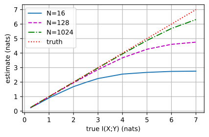
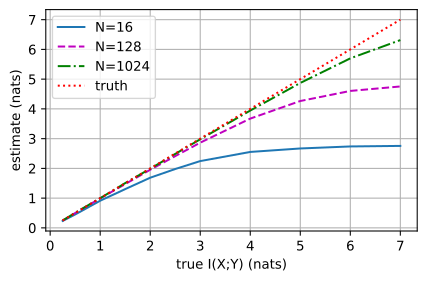
Each curve follows the diagonal while the true mutual information is small, then bends flat as it approaches its ceiling \(\ln N\) (\(\approx 2.77\), \(4.85\), and \(6.93\) nats for the three batch sizes), even though the critic is exact. Changing the architecture or optimizing the critic more accurately cannot raise this estimator’s range; increasing \(N\) raises it only logarithmically. This is InfoNCE’s estimator-specific saturation, distinct from the more general order-level result above.
The distinction matters in practice. A reported variational lower bound need not be an accurate measurement of MI. It may nevertheless be a useful training objective: improving a valid but loose bound can shape representations even when the bound remains far below the true information.
28.3.3 Variational Bounds and InfoNCE
Mutual information involves the unknown densities of Equation 28.3.3, which usually cannot be evaluated directly from samples. Variational methods instead bound it from below using samples and an auxiliary model (a “decoder” or a “critic”), then tighten the bound by optimizing that model. This converts one estimation problem into an optimization problem, while introducing approximation and finite-sample error. Contrastive methods use the resulting lower bound as a training objective. We derive three classical bounds and then InfoNCE; Poole et al. (2019) provide a unified treatment.
28.3.3.1 The Barber–Agakov Bound
The first bound replaces the unknown posterior with a model of it.
Proposition (Barber–Agakov bound). For any conditional density \(q(x \mid y)\),
\[I(X; Y) \geq H(X) + E_{(x,y) \sim P_{X,Y}}\left[\log q(x \mid y)\right], \tag{28.3.8}\]
with equality if and only if \(q(x \mid y) = p(x \mid y)\).
Proof. Write \(I(X; Y) = H(X) - H(X \mid Y)\) and insert the model:
\[ I(X; Y) - H(X) - E\left[\log q(x \mid y)\right] = E\left[\log \frac{p(x \mid y)}{q(x \mid y)}\right] = E_{y}\left[D_{\textrm{KL}}\!\left(p(\cdot \mid y) \,\|\, q(\cdot \mid y)\right)\right] \geq 0 \]
by Gibbs’ inequality, applied for each value of \(y\) and averaged. Equality holds iff the per-\(y\) divergences all vanish, i.e., \(q\) is the posterior. \(\blacksquare\)
The bound (Barber and Agakov 2003) is the information-theoretic reading of an encoder–decoder: if a decoder can reconstruct \(X\) from \(Y\) with low cross-entropy, the pair must share a lot of information. Its weakness is the \(H(X)\) term, which is unknown in exactly the situations where we need the bound (though it is a constant: maximizing the bound never needs it). The same proof with \(q(x \mid y)/p(x)\) in place of \(q(x \mid y)\) gives the equivalent ratio form \(I \geq E[\log\left(q(x \mid y)/p(x)\right)]\), which we will reuse for InfoNCE.
28.3.3.2 Donsker–Varadhan and MINE
The second bound dispenses with normalized models altogether: it characterizes KL divergence, hence mutual information, as a supremum over arbitrary critic functions \(T(x, y)\), with no requirement that anything integrate to one. This is the same convex-duality pattern that drives the f-GAN construction in Section 28.2.
Proposition (Donsker–Varadhan representation). For any distributions \(P, Q\) and any function \(T\) with \(E_Q[e^T] < \infty\),
\[D_{\textrm{KL}}(P \| Q) \geq E_P[T] - \log E_Q\left[e^{T}\right], \tag{28.3.9}\]
with equality if and only if \(T = \log \frac{dP}{dQ} + c\) for a constant \(c\); taking the supremum over \(T\) attains \(D_{\textrm{KL}}(P \| Q)\) (both statements for \(P \ll Q\) with finite divergence) (Donsker and Varadhan 1983).
Proof. Given \(T\), define the Gibbs distribution \(g(x) = q(x)\, e^{T(x)} / Z\) with normalizer \(Z = E_Q[e^T]\), the distribution \(Q\) “tilted” by the critic. Then
\[ D_{\textrm{KL}}(P \| Q) - \left(E_P[T] - \log Z\right) = E_P\left[\log \frac{p}{q} - T + \log Z\right] = E_P\left[\log \frac{p}{g}\right] = D_{\textrm{KL}}(P \| G) \geq 0, \]
by Gibbs’ inequality (the eponymous coincidence is no accident). Equality holds iff \(P = G\), i.e., \(p/q = e^{T}/Z\), i.e., \(T = \log(p/q) + \log Z\). \(\blacksquare\)
Specializing \(P = P_{X,Y}\) and \(Q = P_X \otimes P_Y\) bounds mutual information: for any critic \(T(x,y)\),
\[ I(X; Y) \geq E_{P_{X,Y}}[T] - \log E_{P_X \otimes P_Y}\left[e^{T}\right], \]
where the second expectation is estimated by shuffling: pairing each \(x\) with a \(y\) drawn from a different example destroys the dependence and samples the product of marginals. MINE (mutual information neural estimation, Belghazi et al. (2018)) is exactly this bound with \(T\) a neural network trained by gradient ascent on Equation 28.3.9, plus a fix for the subtlety that the \(\log E[e^T]\) term makes naive minibatch gradients biased.
28.3.3.3 The NWJ Bound and the Bias–Variance Spectrum
The logarithm in front of \(E_Q[e^T]\) causes the difficulty: it couples all samples in the batch and gives the DV bound its bias and, at high MI, its exploding variance (the expectation of \(e^T\) under \(Q\) is carried by the same rare events that the McAllester–Stratos argument warned about). The tangent-line inequality \(\log z \leq z/e\) (equality at \(z = e\)) trades tightness for tractability: applying it to \(Z = E_Q[e^T]\) in Equation 28.3.9 gives, for every critic \(T\),
\[I(X; Y) \geq E_{P_{X,Y}}[T] - e^{-1}\, E_{P_X \otimes P_Y}\left[e^{T}\right], \tag{28.3.10}\]
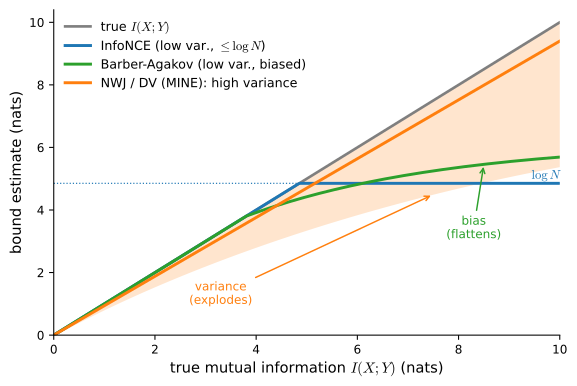
the NWJ bound (Nguyen et al. 2010), tight at \(T^* = 1 + \log\frac{dP}{dQ}\). Since \(e^{-1} E_Q[e^T] = E_Q[e^{T-1}]\), the right-hand side is exactly the f-GAN bound for the KL divergence, \(E_P[T] - E_Q[e^{T-1}]\), that Fenchel duality produced in Section 28.2: this is where we meet that bound again. Because no log-of-average appears, plain minibatch estimates of Equation 28.3.10 are unbiased for the bound itself, but the \(e^{T}\) term still has heavy tails, so the variance problem survives. Figure 28.3.2 sketches the resulting family: estimators stacked under the true value, trading bias for variance, with the contrastive bound we meet next sitting lowest but steadiest.
28.3.3.4 InfoNCE: Estimation as Classification
InfoNCE takes a different route to taming the partition function: it embeds the problem in a classification task, the guessing game we simulated in Section 28.3.2. Draw one positive pair and \(N-1\) negatives, score every candidate with a critic \(f(x, y)\), and ask a softmax to point at the positive. The InfoNCE loss (Oord et al. 2018) is the resulting cross-entropy,
\[\mathcal{L}_{\textrm{NCE}} = -E\left[\log \frac{e^{f(x, y_1)}}{\sum_{j=1}^{N} e^{f(x, y_j)}}\right], \tag{28.3.11}\]
where the expectation is over \((x, y_1) \sim P_{X,Y}\) and \(y_2, \ldots, y_N \sim P_Y\) i.i.d., and the associated mutual-information estimator is the batch ceiling minus the loss,
\[\hat{I}_{\textrm{NCE}} = \log N - \mathcal{L}_{\textrm{NCE}}. \tag{28.3.12}\]
(Many papers, following Oord et al. (2018), write the loss with a \(\frac{1}{N}\) inside the logarithm and a compensating \(+\log N\) outside; the two cancel, so that convention and Equation 28.3.11 are the same number.) Note what the loss is: a \(k\)-class categorical cross-entropy with \(k = N\), the same loss dissected in Section 27.3.2.1 and Section 28.1, with classes that are other examples in the batch rather than fixed labels. That is the entire engineering appeal (this loss is exactly what deep-learning libraries optimize best), and it is the loss of CPC, SimCLR, and CLIP-style dual encoders, where \(x\) and \(y\) are two views or two modalities of the same datum and the batch supplies the negatives (Oord et al. 2018; Radford et al. 2021).
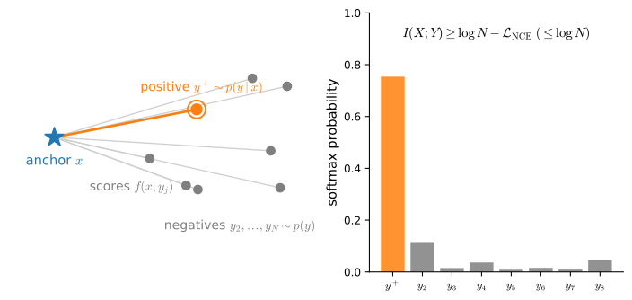
Figure 28.3.3 illustrates the classification problem. The corresponding result is (Poole et al. 2019): small InfoNCE loss certifies mutual information.
Proposition (InfoNCE bound). For any critic \(f\) and any \(N \geq 1\),
\[I(X; Y) \geq \hat{I}_{\textrm{NCE}} = \log N - \mathcal{L}_{\textrm{NCE}}, \qquad \textrm{and } \hat{I}_{\textrm{NCE}} \textrm{ never exceeds } \log N. \tag{28.3.13}\]
Proof. Write \(V = (Y_1, \ldots, Y_N)\) for the whole bag of candidates, where \((X, Y_1) \sim P_{X,Y}\) and the negatives \(Y_{2:N} \sim P_Y\) are independent of \((X, Y_1)\).
Step 1: independent negatives add no information. By the corollary to the chain rule, independent side information adds nothing: \(I(X; V) = I(X; Y_1)\).
Step 2: define a normalized variational model. Define
\[ g(x, v) = \frac{e^{f(x, y_1)}}{\frac{1}{N}\sum_{j=1}^N e^{f(x, y_j)}}. \]
Under the product distribution \(p(x)\,p(v)\), where all \(N\) candidates, including \(y_1\), are i.i.d. draws from \(P_Y\), exchangeability of the \(y_j\) makes each of the \(N\) terms \(E\big[e^{f(x,y_i)} / \frac{1}{N}\sum_j e^{f(x,y_j)}\big]\) equal, so for every fixed \(x\),
\[ E_{p(v)}\left[g(x, V)\right] = \frac{1}{N}\sum_{i=1}^{N} E\left[\frac{e^{f(x, y_i)}}{\frac{1}{N}\sum_{j} e^{f(x, y_j)}}\right] = E\left[\frac{\frac{1}{N}\sum_{i} e^{f(x, y_i)}}{\frac{1}{N}\sum_{j} e^{f(x, y_j)}}\right] = 1. \]
Hence \(q(v \mid x) = p(v)\, g(x, v)\) is a bona fide normalized conditional distribution over bags.
Step 3: Barber–Agakov on the bag. The ratio form of Equation 28.3.8 applied to \((X, V)\) with the model \(q(v \mid x)\) gives
\[ I(X; V) \geq E_{p(x, v)}\left[\log \frac{q(v \mid x)}{p(v)}\right] = E\left[\log g(X, V)\right] = \log N - \mathcal{L}_{\textrm{NCE}}. \]
Combining with Step 1 proves the bound. For the ceiling, the softmax assigns the positive a probability at most \(1\), so \(\mathcal{L}_{\textrm{NCE}} \geq 0\) and the estimator Equation 28.3.12 is at most \(\log N\). \(\blacksquare\)
The two halves of the proposition are the two faces of contrastive learning. The bound explains why it works: driving the classification loss down provably drives shared information up, and the optimal critic recovers the density ratio \(f^*(x,y) = \textrm{pmi}(x,y) + c(x)\) (Exercise 8; (Poole et al. 2019)). With \(N\) candidates, the bound has the exact upper limit \(\log N\). This fact partly motivates the large candidate sets used by CPC, SimCLR, and CLIP, although optimization and negative diversity also matter. One practical hyperparameter deserves attention: in SimCLR-style systems the critic is a scaled cosine similarity between the two embeddings, \(f(x, y) = \textrm{sim}(z_x, z_y)/\tau\), and the temperature \(\tau\) (Chen et al. 2020) is the same knob as the distillation temperature of Section 28.1: lowering \(\tau\) sharpens the softmax over candidates and concentrates the loss on the hardest negatives.
The following experiment compares all three bounds with critics set to their optima using the closed-form Gaussian ratio. The remaining behavior therefore belongs to the bounds, rather than critic optimization. We use a batch of \(N=128\) and report the mean and standard deviation over \(200\) batches.
rng = onp.random.default_rng(3)
N, B = 128, 200
print('true I    DV (MINE)         NWJ              InfoNCE')
for tm in [0.5, 1.0, 2.0, 4.0, 6.0]:
    rho = onp.sqrt(1 - onp.exp(-2 * tm))
    dv, nwj, nce = [], [], []
    for _ in range(B):
        x, y = gauss_pair(rng, rho, N)
        joint = pmi_gauss(x, y, rho)               # T* on positive pairs
        # A random permutation leaves ~1 fixed point per batch of N=128, so
        # one "negative" is secretly a true pair; the O(1/N) contamination
        # is negligible next to the heavy tails probed here.
        prod = pmi_gauss(x, rng.permutation(y), rho)   # T* on shuffled pairs
        dv.append(joint.mean() - onp.log(onp.mean(onp.exp(prod))))
        nwj.append(joint.mean() + 1 - onp.mean(onp.exp(prod)))
        f = pmi_gauss(x[:, None], y[None, :], rho)
        f -= f.max(axis=1, keepdims=True)
        ll = onp.diag(f) - onp.log(onp.exp(f).sum(axis=1))
        nce.append(ll.mean() + onp.log(N))
    print(f'{tm:5.1f}   {onp.mean(dv):6.2f} +-{onp.std(dv):6.2f} '
          f'  {onp.mean(nwj):6.2f} +-{onp.std(nwj):6.2f} '
          f'  {onp.mean(nce):6.2f} +-{onp.std(nce):6.2f}')
true I DV (MINE) NWJ InfoNCE
0.5 0.50 +- 0.12 0.50 +- 0.12 0.50 +- 0.07
1.0 1.01 +- 0.19 0.99 +- 0.22 1.00 +- 0.07
2.0 1.93 +- 0.35 1.83 +- 0.97 1.94 +- 0.09
4.0 3.79 +- 0.92 3.36 +- 1.18 3.67 +- 0.08
6.0 23.22 +- 56.65 1.23 +- 11.74 4.61 +- 0.05The table is Figure 28.3.2 in numbers. At low mutual information all three estimators are accurate and well-behaved. As the truth climbs past \(\ln N \approx 4.85\) nats, they fail in their characteristic ways: InfoNCE stays steady (standard deviation a few hundredths of a nat) but saturates at its ceiling; NWJ’s batch-to-batch spread grows first, exploding to many nats while its mean falls far below the truth; and DV’s log-of-average adds upward bias and the largest blow-up, until single batches return highly unstable values: at a true MI of \(6\) nats its batch estimates average far above the truth with a spread of tens of nats, despite using a perfect critic. Estimator choice is therefore a bias–variance decision, not a ranking.
28.3.3.5 Experiment: Learning the Critic
Finally, let the critic be learned, as in practice. We train a small MLP critic \(f(x, y)\) with the InfoNCE loss on a correlated Gaussian pair with \(\rho = 0.99\), whose true mutual information we know exactly: \(-\tfrac{1}{2}\log(1 - 0.99^2) \approx 1.958\) nats. The data are generated once in NumPy with a fixed seed; training uses batches of \(N = 128\), and we then evaluate the trained critic’s InfoNCE bound at several evaluation batch sizes to examine the \(\log N\) ceiling and its approach to the true value.
rho, n_pool = 0.99, 4096
data_rng = onp.random.default_rng(0)
x_tr, y_tr = (torch.tensor(a, dtype=torch.float32)
              for a in gauss_pair(data_rng, rho, n_pool))
x_ev, y_ev = (torch.tensor(a, dtype=torch.float32)
              for a in gauss_pair(data_rng, rho, n_pool))

torch.manual_seed(0)
critic = torch.nn.Sequential(
    torch.nn.Linear(2, 64), torch.nn.ReLU(),
    torch.nn.Linear(64, 64), torch.nn.ReLU(), torch.nn.Linear(64, 1))
opt = torch.optim.Adam(critic.parameters(), lr=1e-3)

def scores(x, y):
    """Matrix of critic scores f(x_i, y_j) for all pairs in a batch."""
    N = len(x)
    xy = torch.stack([x.reshape(N, 1).expand(N, N),
                      y.reshape(1, N).expand(N, N)], dim=-1)
    return critic(xy.reshape(-1, 2)).reshape(N, N)

N = 128
for step in range(400):
    idx = torch.tensor(data_rng.choice(n_pool, N, replace=False))
    f = scores(x_tr[idx], y_tr[idx])
    loss = (torch.logsumexp(f, dim=1) - f.diag()).mean()
    opt.zero_grad(); loss.backward(); opt.step()

with torch.no_grad():
    for N_ev in [2, 8, 32, 128]:
        vals = [(scores(x_ev[i:i + N_ev], y_ev[i:i + N_ev]).diag()
                 - torch.logsumexp(scores(x_ev[i:i + N_ev],
                                          y_ev[i:i + N_ev]), dim=1)
                 ).mean().item()
                for i in range(0, n_pool, N_ev)]
        print(f'N = {N_ev:4d}: ln N = {onp.log(N_ev):.3f}, '
              f'InfoNCE bound = {onp.log(N_ev) + onp.mean(vals):.3f} nats')
print(f'true I(X;Y) = {-0.5 * onp.log(1 - rho**2):.3f} nats')
N = 2: ln N = 0.693, InfoNCE bound = 0.570 nats
N = 8: ln N = 2.079, InfoNCE bound = 1.407 nats
N = 32: ln N = 3.466, InfoNCE bound = 1.762 nats
N = 128: ln N = 4.852, InfoNCE bound = 1.888 nats
true I(X;Y) = 1.959 natsrho, n_pool = 0.99, 4096
data_rng = onp.random.default_rng(0)
x_tr, y_tr = (a.astype('float32') for a in gauss_pair(data_rng, rho, n_pool))
x_ev, y_ev = (a.astype('float32') for a in gauss_pair(data_rng, rho, n_pool))
tf.random.set_seed(0)
critic = tf.keras.Sequential([
tf.keras.layers.Dense(64, activation='relu'),
tf.keras.layers.Dense(64, activation='relu'), tf.keras.layers.Dense(1)])
opt = tf.keras.optimizers.Adam(1e-3)
def scores(x, y):
"""Matrix of critic scores f(x_i, y_j) for all pairs in a batch."""
N = tf.shape(x)[0]
xy = tf.stack([tf.tile(tf.reshape(x, (-1, 1)), (1, N)),
tf.tile(tf.reshape(y, (1, -1)), (N, 1))], axis=-1)
return tf.reshape(critic(tf.reshape(xy, (-1, 2))), (N, N))
@tf.function
def step(x, y):
with tf.GradientTape() as tape:
f = scores(x, y)
loss = tf.reduce_mean(tf.reduce_logsumexp(f, axis=1)
- tf.linalg.diag_part(f))
grads = tape.gradient(loss, critic.trainable_variables)
opt.apply_gradients(zip(grads, critic.trainable_variables))
N = 128
for s in range(400):
idx = data_rng.choice(n_pool, N, replace=False)
step(tf.constant(x_tr[idx]), tf.constant(y_tr[idx]))
for N_ev in [2, 8, 32, 128]:
vals = []
for i in range(0, n_pool, N_ev):
f = scores(tf.constant(x_ev[i:i + N_ev]),
tf.constant(y_ev[i:i + N_ev]))
vals.append(float(tf.reduce_mean(
tf.linalg.diag_part(f) - tf.reduce_logsumexp(f, axis=1))))
print(f'N = {N_ev:4d}: ln N = {onp.log(N_ev):.3f}, '
f'InfoNCE bound = {onp.log(N_ev) + onp.mean(vals):.3f} nats')
print(f'true I(X;Y) = {-0.5 * onp.log(1 - rho**2):.3f} nats')N = 2: ln N = 0.693, InfoNCE bound = 0.570 nats
N = 8: ln N = 2.079, InfoNCE bound = 1.408 nats
N = 32: ln N = 3.466, InfoNCE bound = 1.765 nats
N = 128: ln N = 4.852, InfoNCE bound = 1.892 nats
true I(X;Y) = 1.959 natsrho, n_pool = 0.99, 4096
data_rng = onp.random.default_rng(0)
x_tr, y_tr = (jnp.array(a, dtype='float32')
for a in gauss_pair(data_rng, rho, n_pool))
x_ev, y_ev = (jnp.array(a, dtype='float32')
for a in gauss_pair(data_rng, rho, n_pool))
def init_mlp(key, sizes=(2, 64, 64, 1)):
params = []
for d_in, d_out in zip(sizes[:-1], sizes[1:]):
key, sub = jax.random.split(key)
params.append((jax.random.normal(sub, (d_in, d_out))
* jnp.sqrt(2 / d_in), jnp.zeros(d_out)))
return params
def scores(params, x, y):
"""Matrix of critic scores f(x_i, y_j) for all pairs in a batch."""
h = jnp.stack(jnp.meshgrid(x, y, indexing='ij'), axis=-1)
for W, b in params[:-1]:
h = jax.nn.relu(h @ W + b)
return (h @ params[-1][0] + params[-1][1])[..., 0]
def loss_fn(params, x, y):
f = scores(params, x, y)
return (jax.scipy.special.logsumexp(f, axis=1) - jnp.diag(f)).mean()
params = init_mlp(jax.random.PRNGKey(0))
opt = optax.adam(1e-3)
state = opt.init(params)
@jax.jit
def step(params, state, x, y):
grads = jax.grad(loss_fn)(params, x, y)
updates, state = opt.update(grads, state)
return optax.apply_updates(params, updates), state
N = 128
for s in range(400):
idx = data_rng.choice(n_pool, N, replace=False)
params, state = step(params, state, x_tr[idx], y_tr[idx])
for N_ev in [2, 8, 32, 128]:
vals = []
for i in range(0, n_pool, N_ev):
f = scores(params, x_ev[i:i + N_ev], y_ev[i:i + N_ev])
vals.append(float((jnp.diag(f)
- jax.scipy.special.logsumexp(f, axis=1)).mean()))
print(f'N = {N_ev:4d}: ln N = {onp.log(N_ev):.3f}, '
f'InfoNCE bound = {onp.log(N_ev) + onp.mean(vals):.3f} nats')
print(f'true I(X;Y) = {-0.5 * onp.log(1 - rho**2):.3f} nats')N = 2: ln N = 0.693, InfoNCE bound = 0.569 nats
N = 8: ln N = 2.079, InfoNCE bound = 1.405 nats
N = 32: ln N = 3.466, InfoNCE bound = 1.756 nats
N = 128: ln N = 4.852, InfoNCE bound = 1.881 nats
true I(X;Y) = 1.959 natsrho, n_pool = 0.99, 4096
data_rng = onp.random.default_rng(0)
x_tr, y_tr = (a.astype('float32') for a in gauss_pair(data_rng, rho, n_pool))
x_ev, y_ev = (a.astype('float32') for a in gauss_pair(data_rng, rho, n_pool))
np.random.seed(0)
critic = gluon.nn.Sequential()
critic.add(gluon.nn.Dense(64, activation='relu'),
gluon.nn.Dense(64, activation='relu'), gluon.nn.Dense(1))
critic.initialize(init.Xavier())
trainer = gluon.Trainer(critic.collect_params(), 'adam',
{'learning_rate': 1e-3})
def scores(x, y):
"""Matrix of critic scores f(x_i, y_j) for all pairs in a batch."""
N = x.shape[0]
xy = np.stack([np.tile(x.reshape(-1, 1), (1, N)),
np.tile(y.reshape(1, -1), (N, 1))], axis=-1)
return critic(xy.reshape(-1, 2)).reshape(N, N)
def diag_minus_logsumexp(f):
"""Per-row log-softmax of the diagonal (positive-pair) scores."""
m = f.max(axis=1, keepdims=True)
lse = (m + np.log(np.exp(f - m).sum(axis=1, keepdims=True)))[:, 0]
return (f * np.eye(f.shape[0])).sum(axis=1) - lse
N = 128
for step in range(400):
idx = data_rng.choice(n_pool, N, replace=False)
x, y = np.array(x_tr[idx]), np.array(y_tr[idx])
with autograd.record():
loss = -diag_minus_logsumexp(scores(x, y)).mean()
loss.backward()
trainer.step(1)
for N_ev in [2, 8, 32, 128]:
vals = [float(diag_minus_logsumexp(
scores(np.array(x_ev[i:i + N_ev]),
np.array(y_ev[i:i + N_ev]))).mean())
for i in range(0, n_pool, N_ev)]
print(f'N = {N_ev:4d}: ln N = {onp.log(N_ev):.3f}, '
f'InfoNCE bound = {onp.log(N_ev) + onp.mean(vals):.3f} nats')
print(f'true I(X;Y) = {-0.5 * onp.log(1 - rho**2):.3f} nats')[22:57:18] /home/smola/mxnet/src/base.cc:48: GPU context requested, but no GPUs found.N = 2: ln N = 0.693, InfoNCE bound = 0.570 nats
N = 8: ln N = 2.079, InfoNCE bound = 1.408 nats
N = 32: ln N = 3.466, InfoNCE bound = 1.764 nats
N = 128: ln N = 4.852, InfoNCE bound = 1.891 nats
true I(X;Y) = 1.959 natsIn this controlled evaluation, the trained critic and data pool are fixed while the number of negatives changes. At \(N=2\), InfoNCE cannot exceed \(\ln2\); at \(N=8\), the ceiling exceeds the true \(1.958\) nats but the learned bound remains about \(1.4\); by \(N=128\), it reaches about \(1.89\). The negative count therefore sets InfoNCE’s exact upper range here, but it is not the sole determinant of the result: critic approximation, optimization, in-batch dependence, and finite evaluation data also contribute.
28.3.4 The Information Bottleneck and the Limits of Mutual Information
We close with the principle that joins this section’s two themes (what representations preserve and what we can measure) into a single objective, and with an assessment of where its empirical support stands.
28.3.4.1 The Information-Bottleneck Lagrangian
What makes a representation \(Z\) of an input \(X\) good for predicting a label \(Y\)? The information bottleneck (IB) principle (Tishby et al. 1999) answers with two mutual informations: a good \(Z\) keeps little of \(X\) (it compresses) while keeping much of \(Y\) (it predicts). Over stochastic encoders \(p(z \mid x)\), minimize the Lagrangian
\[\min_{p(z \mid x)}\; I(X; Z) - \beta\, I(Y; Z). \tag{28.3.14}\]
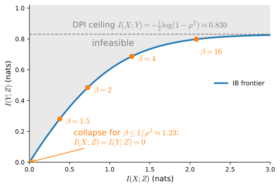
The data-processing inequality is what makes this well-posed: since \(Y \to X \to Z\) is a Markov chain (the encoder sees only \(X\)), we always have \(I(Y; Z) \leq \min\{I(X; Y),\, I(X; Z)\}\): the representation can never know more about the label than the input does, and predicting well forces \(Z\) to retain input information. The multiplier \(\beta\) sets the tradeoff. In finite/discrete settings, or in stochastic encoder families where optima exist, the \(\beta\to0\) limit favors a constant representation. Large \(\beta\) prioritizes predictive information; recovering a minimal sufficient statistic additionally requires that one lie in the encoder family and that the relevant optimum be attained. For deterministic continuous encoders, \(I(X;Z)\) can be infinite, which is one reason the stochastic formulation matters. Sweeping \(\beta\) traces an attainable frontier in the information plane with coordinates \((I(X;Z),I(Y;Z))\) for the chosen family. Rate–distortion theory (Shannon 1959) is the special case where “relevance” is a hand-chosen distortion measure; IB lets the label define relevance instead. The deep variational information bottleneck (VIB) (Alemi et al. 2017) makes Equation 28.3.14 trainable by applying the bounds derived above to both terms: a Barber–Agakov-style decoder bound for \(I(Y;Z)\) from below and a variational upper bound for \(I(X;Z)\). That is the same replace-the-intractable-posterior pattern as the ELBO of Section 27.3.5, and another reminder that in deep learning, mutual informations are optimized through bounds, not computed. The frontier this tradeoff traces is shown in Figure 28.3.4.
28.3.4.2 The Information Plane: a Gaussian Bottleneck in Closed Form
Rather than train a VIB (two stacked variational bounds would put us two bounds away from anything checkable), we exhibit the IB tradeoff in a model where every quantity is exact (Chechik et al. 2005). Let \((X, Y)\) be our standard Gaussian pair with \(\rho = 0.9\), so \(I(X; Y) \approx 0.830\) nats, and let the encoder be a noisy channel
\[ Z = X + \sigma\, \epsilon, \qquad \epsilon \sim \mathcal{N}(0, 1), \]
with the noise scale \(\sigma\) as the compression knob. Both informations follow from the Gaussian anchor Equation 28.3.4: the correlations are \(\rho_{XZ}^2 = 1/(1 + \sigma^2)\) and \(\rho_{YZ}^2 = \rho^2/(1 + \sigma^2)\), so
\[ I(X; Z) = \tfrac{1}{2}\log\left(1 + \sigma^{-2}\right), \qquad I(Y; Z) = -\tfrac{1}{2}\log\left(1 - \frac{\rho^2}{1 + \sigma^2}\right). \]
In this scalar Gaussian family the noise level is the only degree of freedom, so sweeping \(\sigma\) traces the family’s entire curve; the Gaussian information bottleneck theorem of (Chechik et al. 2005) adds that this curve is the optimal frontier over all encoders \(p(z \mid x)\). Minimizing the Lagrangian Equation 28.3.14 over \(\sigma\) for each \(\beta\) picks out one operating point on the frontier.
rho = 0.9
sigma = onp.logspace(-2, 2, 401)            # noise scale: the beta knob
I_xz = 0.5 * onp.log(1 + sigma**-2)         # compression cost
I_yz = -0.5 * onp.log(1 - rho**2 / (1 + sigma**2))  # predictive value
I_xy = -0.5 * onp.log(1 - rho**2)

d2l.plot(I_xz, [I_yz, onp.full_like(I_xz, I_xy)], 'I(X;Z) (nats)',
         'I(Y;Z) (nats)', legend=['IB frontier', 'I(X;Y) ceiling'],
         xlim=[0, 3], figsize=(5, 3))
for beta in [1.0, 1.5, 2.0, 4.0, 16.0]:
    i = onp.argmin(I_xz - beta * I_yz)      # IB Lagrangian on the grid
    d2l.plt.plot(I_xz[i], I_yz[i], 'ro')
    d2l.plt.annotate(f'{beta:g}', (I_xz[i], I_yz[i]),
                     textcoords='offset points', xytext=(6, -2))
    print(f'beta = {beta:4.1f}: I(X;Z) = {I_xz[i]:.3f}, '
f'I(Y;Z) = {I_yz[i]:.3f} nats')beta = 1.0: I(X;Z) = 0.000, I(Y;Z) = 0.000 nats
beta = 1.5: I(X;Z) = 0.382, I(Y;Z) = 0.284 nats
beta = 2.0: I(X;Z) = 0.731, I(Y;Z) = 0.487 nats
beta = 4.0: I(X;Z) = 1.283, I(Y;Z) = 0.689 nats
beta = 16.0: I(X;Z) = 2.080, I(Y;Z) = 0.798 nats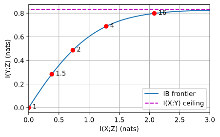
beta =  1.0: I(X;Z) = 0.000, I(Y;Z) = 0.000 nats
beta =  1.5: I(X;Z) = 0.382, I(Y;Z) = 0.284 nats
beta =  2.0: I(X;Z) = 0.731, I(Y;Z) = 0.487 nats
beta =  4.0: I(X;Z) = 1.283, I(Y;Z) = 0.689 nats
beta = 16.0: I(X;Z) = 2.080, I(Y;Z) = 0.798 nats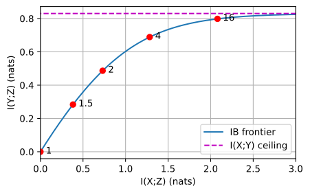
beta =  1.0: I(X;Z) = 0.000, I(Y;Z) = 0.000 nats
beta =  1.5: I(X;Z) = 0.382, I(Y;Z) = 0.284 nats
beta =  2.0: I(X;Z) = 0.731, I(Y;Z) = 0.487 nats
beta =  4.0: I(X;Z) = 1.283, I(Y;Z) = 0.689 nats
beta = 16.0: I(X;Z) = 2.080, I(Y;Z) = 0.798 nats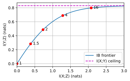
beta =  1.0: I(X;Z) = 0.000, I(Y;Z) = 0.000 nats
beta =  1.5: I(X;Z) = 0.382, I(Y;Z) = 0.284 nats
beta =  2.0: I(X;Z) = 0.731, I(Y;Z) = 0.487 nats
beta =  4.0: I(X;Z) = 1.283, I(Y;Z) = 0.689 nats
beta = 16.0: I(X;Z) = 2.080, I(Y;Z) = 0.798 nats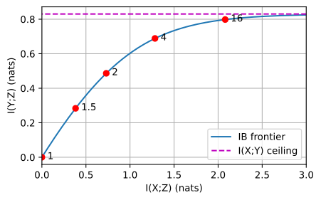
The frontier rises steeply from the origin (the first fraction of a nat of retained input information increases label information at the best exchange rate, \(\rho^2\) nats per nat), then flattens as \(I(Y;Z)\) approaches its DPI ceiling \(I(X;Y)\): retaining more of \(X\) yields progressively less additional information about \(Y\). The marked points show the \(\beta\) knob at work, including the degenerate regime: for \(\beta \leq 1/\rho^2 \approx 1.23\) the exchange rate never beats the price and the optimum is the origin, \(I(X;Z) = I(Y;Z) = 0\); beyond it, rising \(\beta\) moves the operating point up the frontier. A deep VIB approximates this construction on real data using encoder noise instead of \(\sigma\) and variational bounds instead of closed forms. Its \(\beta\)-sweep traces a noisy version of the same curve.
28.3.4.3 The Compression-Phase Debate
The information plane has also been central to a debate about deep learning. Shwartz-Ziv and Tishby (2017) plotted estimated \((I(X;Z), I(Y;Z))\) trajectories of ordinary classifiers during training and reported a two-phase dynamic, a fast fitting phase (both informations rise) followed by a long compression phase (\(I(X;Z)\) falls while \(I(Y;Z)\) holds), proposed as the mechanism by which deep networks generalize. Saxe et al. (2018) re-examined the claim and found the compression phase to be largely an artifact: it appears with saturating activations (tanh squashes activations into the bins’ edges, which the binned MI estimator reads as compression) and disappears with ReLU networks, which can generalize without any measured compression. Moreover, for a deterministic network with continuous inputs, \(I(X; Z)\) is in fact infinite or constant (the singular case flagged at the definition Equation 28.3.3): whatever the plotted trajectories track, it is a property of the binning, not a mutual information. Where the debate stands: the IB objective Equation 28.3.14 is well-posed for explicitly stochastic encoders and trains well (VIB improves robustness and calibration in practice), but the claim that standard training implicitly performs IB compression remains unsettled. The debate illustrates the difficulty of interpreting MI estimates.
28.3.4.4 What Mutual Information Guarantees: Fano’s Inequality
One guarantee explains why anyone wants high mutual information in the first place: enough shared information is a prerequisite for accurate prediction.
Proposition (Fano’s inequality). Let \(X\) take values in a set of size \(k\), and let \(\hat{X} = g(Y)\) be any estimate of \(X\) computed from \(Y\), with error probability \(P_e = P(\hat{X} \neq X)\). Then
\[H_b(P_e) + P_e \log(k - 1) \geq H(X \mid Y) = H(X) - I(X; Y), \tag{28.3.15}\]
where \(H_b\) is the binary entropy in nats (Cover and Thomas 1999).
Proof. Let \(E = \mathbf{1}_{\hat{X} \neq X}\) be the error indicator and expand \(H(E, X \mid \hat{X})\) by the chain rule in both orders. One order: \(H(E, X \mid \hat{X}) = H(X \mid \hat{X})\), since \(E\) is a function of \((X, \hat{X})\). The other: \(H(E, X \mid \hat{X}) = H(E \mid \hat{X}) + H(X \mid E, \hat{X}) \leq H_b(P_e) + P_e \log(k-1)\), because conditioning cannot raise entropy (\(H(E \mid \hat{X}) \leq H(E) = H_b(P_e)\), since \(I(E; \hat{X}) \geq 0\)), and given \(E\): when \(E = 0\), \(X = \hat{X}\) is known (zero entropy), and when \(E = 1\) (probability \(P_e\)), \(X\) ranges over at most \(k - 1\) values. Finally \(X \to Y \to \hat{X}\) is a Markov chain, so the data-processing inequality gives \(I(X; \hat{X}) \leq I(X; Y)\), i.e., \(H(X \mid \hat{X}) \geq H(X \mid Y)\). Chaining the three displays proves the claim. \(\blacksquare\)
Fano converts information into a floor on achievable error: no representation, classifier, or amount of compute can beat it. It quantifies the “prerequisite” reading of contrastive learning: features that support accurate downstream classification must carry high mutual information with the label. Combining this requirement with the estimation ceiling gives:
k, p_e = 1000, 0.05
H_b = lambda p: -p * onp.log(p) - (1 - p) * onp.log(1 - p)
need = onp.log(k) - H_b(p_e) - p_e * onp.log(k - 1)
print(f'{p_e:.0%} error on {k} balanced classes needs '
      f'I(X;Y) >= {need:.3f} nats')
print(f'InfoNCE can reach that value only if N >= e^I = {onp.exp(need):.0f}')
5% error on 1000 balanced classes needs I(X;Y) >= 6.364 nats
InfoNCE can reach that value only if N >= e^I = 581Five percent error on a thousand balanced classes requires at least \(6.36\) nats of label information. Since InfoNCE cannot exceed \(\log N\), it can reach that numerical value only when \(N\geq e^{6.36}\approx581\). This is a necessary range condition for InfoNCE, not a universal sample-size threshold for every estimator or confidence procedure.
28.3.4.5 What Mutual Information Estimates Establish
The preceding results suggest several guidelines for interpreting mutual information estimates.
- Separate estimates, bounds, and confidence guarantees. InfoNCE, NWJ, DV/MINE, and decoder objectives are variational bounds evaluated with finite samples and often imperfect critics. Histogram, kernel, and nearest-neighbor methods are point estimators with different bias and tuning problems. The general \(O(\log N)\) theorem concerns distribution-free high-confidence lower guarantees; it does not give every point estimator an exact range. InfoNCE has its own exact \(\log N\) cap, whereas empirical DV and NWJ values are unbounded and can become extremely variable.
- A useful objective need not provide an accurate estimate. Tschannen et al. (2020) show that downstream representation quality correlates poorly with the tightness of the MI bound being maximized: looser bounds sometimes yield better representations, and InfoNCE’s success owes as much to the inductive biases of the critic architecture and the choice of views as to its information content. Maximizing an MI bound can therefore be a useful training signal without providing a reliable numerical estimate of mutual information.
- Invariances complicate estimation. MI’s reparameterization invariance provides a broad notion of dependence but makes estimation difficult; any pipeline that needs a trustworthy dependence number on high-dimensional data should confront that tension directly (e.g., by validating its estimator on a known-MI synthetic pair, as we did here).
- The formal guarantees remain useful. The definitions and their calculus, the data-processing inequality, Fano’s floor, the bounds’ validity as bounds, and the closed-form anchors used to test estimators provide a sound basis for analysis, even when high-dimensional numerical estimates are difficult to interpret.
28.3.5 Summary
- Mutual information \(I(X;Y) = D_{\textrm{KL}}(P_{X,Y} \| P_X \otimes P_Y)\) measures how far a pair of variables is from independence. It is symmetric, non-negative, zero exactly at independence, equals \(H(X) - H(X \mid Y) = H(X) + H(Y) - H(X,Y)\), and is invariant under invertible reparameterization of either variable; unlike correlation, it detects any dependence.
- The Gaussian pair gives the closed-form anchor \(I = -\tfrac{1}{2}\log(1 - \rho^2)\); pointwise mutual information scores individual co-occurrences and powers collocation mining in NLP.
- The chain rule \(I(X; Y, Z) = I(X;Z) + I(X; Y \mid Z)\) yields the data-processing inequality: along a Markov chain \(X \to Y \to Z\), \(I(X;Z) \leq I(X;Y)\). Processing never creates information; representations only lose it.
- Estimating MI is statistically hard: any distribution-free, high-confidence lower guarantee from \(N\) samples grows at most on the order of \(\log N\) (McAllester–Stratos). Separately, InfoNCE has an exact \(\log N\) cap even with an ideal critic.
- Practical estimators are variational lower bounds: Barber–Agakov (decoder), Donsker–Varadhan/MINE and NWJ (critics), and InfoNCE (contrastive classification, a categorical cross-entropy). InfoNCE certifies \(I \geq \log N - \mathcal{L}\), is low-variance but saturates at \(\log N\); DV/NWJ are tighter in expectation but their variance explodes at high MI.
- The information bottleneck \(\min I(X;Z) - \beta\, I(Y;Z)\) frames good representation as a compression–prediction tradeoff, made trainable by the same variational bounds (VIB); the claim that ordinary training implicitly compresses is contested (Saxe et al.). Fano’s inequality is the guarantee that survives: low prediction error requires high mutual information.
28.3.6 Exercises
- Prove the discrete bounds \(\max\{H(X), H(Y)\} \leq H(X, Y) \leq H(X) + H(Y)\) from the chain rule and the properties of (conditional) entropy. Which inequality fails for differential entropy, and why?
- Compute \(I(X;Y)\) by hand for the joint p.m.f. \(p_{X,Y} = \left(\begin{smallmatrix} 0.3 & 0.2 \\ 0.1 & 0.4
\end{smallmatrix}\right)\): form the marginals, evaluate the pointwise mutual information at each cell, and average. Check your answer against the
mutual_informationfunction. - Derive the Gaussian formula Equation 28.3.4 directly by integrating Equation 28.3.3 (without the entropy identities). How large must \(\rho\) be for \(I(X;Y)\) to exceed the certification ceiling of a batch of \(N = 256\)?
- Construct a pair of discrete random variables with zero correlation but positive mutual information, and verify both numerically. Then prove that for jointly Gaussian variables, zero correlation does imply \(I = 0\).
- (Data-processing) Let \(X \to Y \to Z\) with a deterministic second step \(Z = g(Y)\). Show \(I(X; g(Y)) \leq I(X; Y)\) with equality when \(g\) is invertible, and give an example where \(g\) is not invertible yet equality still holds. Can post-processing by any randomized \(g\) ever increase mutual information?
- (Synergy) Conditioning can create dependence: let \(X, Y\) be independent fair bits and \(Z = X \oplus Y\) (exclusive or). Show \(I(X; Y) = 0\) but \(I(X; Y \mid Z) = \ln 2\). Why does this not contradict the data-processing inequality?
- Derive the Barber–Agakov bound Equation 28.3.8 from \(I = H(X) - H(X \mid Y)\) and Gibbs’ inequality, and show that the gap of the bound equals \(E_y[D_{\textrm{KL}}(p(\cdot \mid y) \| q(\cdot \mid y))]\).
- Show from Equation 28.3.11 that \(\mathcal{L}_{\textrm{NCE}} \geq 0\), conclude that the InfoNCE estimator Equation 28.3.12 can never exceed \(\log N\), and explain in one paragraph why increasing the batch size tightens the bound. What does the optimal critic look like?
- For the scalar Gaussian bottleneck, derive the critical value \(\beta^* = 1/\rho^2\) below which the IB optimum collapses to an uninformative \(Z\), by examining the slope of the frontier at \(I(X;Z) = 0\). Characterize the optimal \(Z\) as \(\beta \to \infty\).
- Using Fano’s inequality Equation 28.3.15 and the \(\log N\) ceiling taken at face value, estimate the smallest contrastive batch size that could in principle certify enough mutual information for \(1\%\) error on a balanced \(10{,}000\)-class problem. Then design (and run) a sanity check for any MI estimator using a known-MI Gaussian pair.