torch.set_float32_matmul_precision('high') # tf32 matmuls on tensor cores17.7 Few-Step Generation
Every sample from the models of this chapter costs many evaluations of a network. Section 17.4 brought the thousand steps of the ancestral chain down to about fifty, and Section 17.6 made each evaluation cheaper; the generator of a GAN in Chapter 16 needed one. The obvious shortcut, a single Euler step of the probability-flow ODE, fails even with an exact velocity field: every sample lands on the mean of the data, the average that Section 16.7 met in one-step students and escaped by adding a critic.
This section asks what a network must learn instead so that one or two evaluations suffice without a critic. The answer is to learn the solution of the ODE instead of its right-hand side. A flow map takes a point at one time directly to where its trajectory is at an earlier time. Song et al. (2023) learned the jump to the data from the trajectories of a trained diffusion model and called the result a consistency model. Geng et al. (2025) learned the average velocity over any interval with no trained model at all, from an identity that the flow map satisfies.
A flow map keeps the bijection between noise and samples, so inversion and editing work as in Section 17.4, and training remains a regression with one network. We look at the failure on the running example, derive one loss for consistency models and MeanFlow, test it on the mixture and on Fashion-MNIST, and end with the route that matches distributions instead.
17.7.1 Why One Step Fails
A long Euler step makes two errors. It aims where the trajectory points at its start, and it ignores how the trajectory bends on the way. Both can be seen on the mixture with the exact field, where no network error hides them.
17.7.1.1 The Average Where the Data Are Not
One Euler step from pure noise sends every start to the data mean (Section 17.2), for the mixture \((-0.5, -0.7)\), where no data lie.
More steps help, but how many are needed? mix.velocity evaluates the exact field of the mixture, and d2l.make_pred turns it into the predictor that d2l.ode_sample integrates. We run Euler’s method with 1, 2, 4 and 10 steps from the same 20,000 Gaussian starts.
device = d2l.try_gpu()
mix = d2l.GaussianMixture.three_modes(device)
lin = d2l.GaussianPath.linear()
pred_exact = d2l.make_pred(mix.velocity, lin, 'velocity')
torch.manual_seed(0)
z = torch.randn(20_000, 2, device=device)
euler = {n: d2l.ode_sample(pred_exact, z, lin.sigma_bars(n))
         for n in (1, 2, 4, 10)}
for n, x in euler.items():
    s = mix.summary(x)
    print(f'{n:2d} Euler steps: weights {s["weights"]}, stray {s["stray"]:.1%}')
d2l.scatter_panels([x[:2000] for x in euler.values()],
                   [f'{n} steps' for n in euler], data=mix.sample(2000),
                   size=2.4);
1 Euler steps: weights [1.0, 0.0, 0.0], stray 100.0%
2 Euler steps: weights [0.644, 0.217, 0.14], stray 25.1%
4 Euler steps: weights [0.54, 0.277, 0.183], stray 6.5%
10 Euler steps: weights [0.512, 0.291, 0.197], stray 2.2%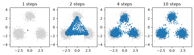
mix = d2l.GaussianMixture.three_modes()
lin = d2l.GaussianPath.linear()
pred_exact = d2l.make_pred(mix.velocity, lin, 'velocity')
z = jax.random.normal(jax.random.key(0), (20_000, 2))
euler = {n: d2l.ode_sample(pred_exact, z, lin.sigma_bars(n))
         for n in (1, 2, 4, 10)}
for n, x in euler.items():
    s = mix.summary(x)
    print(f'{n:2d} Euler steps: weights {s["weights"]}, stray {s["stray"]:.1%}')
d2l.scatter_panels([x[:2000] for x in euler.values()],
                   [f'{n} steps' for n in euler],
                   data=mix.sample(jax.random.key(1), 2000), size=2.4);
1 Euler steps: weights [1.0, 0.0, 0.0], stray 100.0%
2 Euler steps: weights [0.644, 0.221, 0.135], stray 25.2%
4 Euler steps: weights [0.54, 0.278, 0.182], stray 6.6%
10 Euler steps: weights [0.511, 0.293, 0.196], stray 2.3%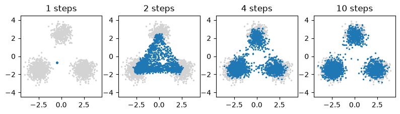
One step puts every sample on the mean, farther than three standard deviations from every mode, so all of them stray. Two steps reach the modes but leave about a quarter of the samples between them, with weights of about 0.64/0.22/0.14 instead of 0.5/0.3/0.2: the heaviest mode gains because the mean lies nearest to it. Four steps still leave about 6.5% of the samples stray, and ten steps about 2%.
17.7.1.2 Straighter Paths Help but Do Not Finish
Why do the trajectories bend at all? Each training example joins a data point to an independently drawn noise vector by a straight segment, but the segments of different examples cross. Where they cross, the field averages their directions, and the trajectories, which cannot cross, bend around each other (Section 43.6.2). The curvature comes from the pairing of noise with data, not from the loss.
Reflow (Liu et al. 2023) changes the pairing. It pairs each noise vector with the sample that a trained model reaches from it and trains the network again on these pairs, whose segments rarely cross. Section 43.6.2.3 proves that a round of reflow keeps the data distribution and never increases the transport cost, and on two-moons data one Euler step of the reflowed model scores as well as thirty-two steps of the original.
Straightening does not finish the job. The reflowed model inherits the original’s errors, each round costs a training run, and on images Liu et al. (2023) still followed reflow with distillation for their one-step results. The rest of this section changes what the network outputs instead of how the data are paired.
17.7.2 Flow Maps
A velocity model says which way a trajectory points; a flow map says where it arrives.
17.7.2.1 The Integral of the Velocity
Run the probability-flow ODE \(d\mathbf{x}_\tau / d\tau = \mathbf{u}_\tau(\mathbf{x}_\tau)\) from a point \(\mathbf{x}\) at time \(t\) back to an earlier time \(s \leq t\). The point where it arrives is the flow map \(\Phi_{t \to s}(\mathbf{x})\). For a field that is Lipschitz in \(\mathbf{x}\) the flow map is a bijection (Section 43.1.1). The sampler we want is \(\Phi_{1 \to 0}\).
Integrating the ODE along the trajectory \(\mathbf{x}_\tau\) through \(\mathbf{x}_t\) writes the flow map as a displacement,
\[\Phi_{t \to s}(\mathbf{x}_t) = \mathbf{x}_t - \int_s^t \mathbf{u}_\tau(\mathbf{x}_\tau)\, d\tau = \mathbf{x}_t - (t - s)\, \bar{\mathbf{u}}(\mathbf{x}_t, s, t), \tag{17.7.1}\]
where \(\bar{\mathbf{u}}(\mathbf{x}_t, s, t)\) is the average velocity along the trajectory between the two times. Euler’s method replaces it by the velocity at the start, \(\mathbf{u}_t(\mathbf{x}_t)\), with an error that grows with the step (Section 43.1.3). Over an interval of length zero the two agree, \(\bar{\mathbf{u}}(\mathbf{x}, t, t) = \mathbf{u}_t(\mathbf{x})\), so a network for \(\bar{\mathbf{u}}\) is a velocity model with one more input, the end time.
The smallest case shows what the average velocity knows that the velocity does not. Let the data be one-dimensional and Gaussian with mean \(m\) and standard deviation \(\varsigma\). Then \(x_t\) is Gaussian with mean \((1 - t)\, m\) and standard deviation \(k_t = \sqrt{(1 - t)^2 \varsigma^2 + t^2}\), and the flow keeps each point’s standardized position \((x - (1 - t) m) / k_t\), so the flow map is affine:
\[\Phi_{t \to s}(x) = (1 - s)\, m + \frac{k_s}{k_t} \big(x - (1 - t)\, m\big).\]
With \(m = 2\) and \(\varsigma = 0.5\) the full jump \(\Phi_{1 \to 0}(x) = 2 + 0.5\, x\) sends standard Gaussian noise to the data \(\mathcal{N}(2, 0.5^2)\), with average velocity \(\bar{u}(x, 0, 1) = 0.5\, x - 2\). The velocity at the start is \(u_1(x) = x - 2\), and its Euler step returns 2 for every \(x\). The average velocity removes only half of the noise, because half of the noise’s spread must survive as the spread of the data.
Three identities characterize the flow map, and each gives a way to train one (Figure 17.7.1). Let \(\mathbf{x}_\tau\) be the trajectory through \(\mathbf{x}\) at time \(t\), and \(s \leq r \leq t\). The compositional identity says that two jumps make one, \(\Phi_{r \to s}(\Phi_{t \to r}(\mathbf{x})) = \Phi_{t \to s}(\mathbf{x})\). The Lagrangian identity fixes the start and moves the end: the mapped point moves with the field, like a particle, \(\partial_s \Phi_{t \to s}(\mathbf{x}) = \mathbf{u}_s(\Phi_{t \to s}(\mathbf{x}))\). The Eulerian identity fixes the end and moves the start along the trajectory: every point of one trajectory maps to the same place,
\[\frac{d}{dt} \Phi_{t \to s}(\mathbf{x}_t) = \partial_t \Phi_{t \to s}(\mathbf{x}_t) + \nabla_{\mathbf{x}} \Phi_{t \to s}(\mathbf{x}_t)\, \mathbf{u}_t(\mathbf{x}_t) = \mathbf{0}. \tag{17.7.2}\]
In the Gaussian example all three can be checked by hand: the ratios \(k_s / k_t\) compose, and the standardized position is constant along a trajectory.
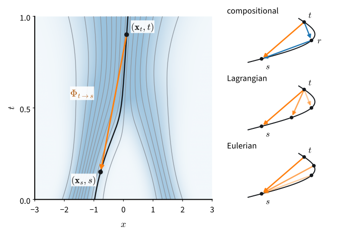
Together with the condition at \(s = t\), where the map is the identity and its slope in \(s\) is the velocity, each identity determines the flow map. Composition needs only the model at an intermediate time; progressive distillation (Salimans and Ho 2022) and shortcut models (Frans et al. 2025) use it. The Lagrangian identity needs the velocity at the output of the map. The Eulerian identity needs the derivative along the trajectory through the input, one Jacobian-vector product. Boffi et al. (2025) sort the few-step methods by the identity they enforce; both methods of this section are Eulerian.
17.7.2.2 Consistency Models
The first flow-map method kept only the jump to the data. A consistency model (Song et al. 2023) is a network \(f(\mathbf{x}, t)\) trained to output \(\Phi_{t \to 0}(\mathbf{x})\) at every time. Its training condition is that the output does not change as the input moves along a trajectory, \(\frac{d}{dt} f(\mathbf{x}_t, t) = \mathbf{0}\) with \(f(\mathbf{x}, 0) = \mathbf{x}\), the Eulerian identity Equation 17.7.2 at \(s = 0\).
In consistency distillation, Song et al. let a trained diffusion model, the teacher, take one ODE step between neighbouring times of a grid, and require the student’s outputs at the two points to agree, with the output at the earlier point held fixed as the target. As the grid is refined the difference, divided by the step, becomes the derivative above, which Lu and Song (2025) use directly. Consistency training replaces the teacher’s velocity by the conditional velocity of each example.
One evaluation of a consistency model gives a sample. A second cannot jump from \(t = 1\) to \(t = 0.5\), because the model knows only where trajectories end. It re-noises instead: the sample is moved back to \(t = 0.5\) with fresh noise, \(\mathbf{x}_{0.5} = 0.5\, \mathbf{x}_0 + 0.5\, \boldsymbol\epsilon'\), and mapped to the data again, from where trajectories bend less. A flow map with both times needs no re-noising: two evaluations are two jumps along one trajectory, and the bijection between noise and samples survives.
17.7.2.3 Average Velocity and the MeanFlow Identity
Writing the flow map through the average velocity Equation 17.7.1 turns the Eulerian identity into a regression target. Multiply the average velocity by the length of its interval, which gives the integral of the velocity, and differentiate in \(t\) along the trajectory with \(s\) held fixed:
\[\frac{d}{dt} \Big[(t - s)\, \bar{\mathbf{u}}(\mathbf{x}_t, s, t)\Big] = \frac{d}{dt} \int_s^t \mathbf{u}_\tau(\mathbf{x}_\tau)\, d\tau = \mathbf{u}_t(\mathbf{x}_t).\]
The product rule on the left gives the MeanFlow identity of Geng et al. (2025),
\[\bar{\mathbf{u}}(\mathbf{x}_t, s, t) = \mathbf{u}_t(\mathbf{x}_t) - (t - s)\, \frac{d}{dt} \bar{\mathbf{u}}(\mathbf{x}_t, s, t). \tag{17.7.3}\]
The average velocity is the velocity at the start, corrected by how fast the average changes as the start slides along the trajectory. Substituting Equation 17.7.1 into Equation 17.7.2 shows that the two identities are the same. The total derivative is \(\partial_t \bar{\mathbf{u}} + (\nabla_{\mathbf{x}} \bar{\mathbf{u}})\, \mathbf{u}_t\), the Jacobian-vector product of the network \((\mathbf{x}, t) \mapsto \bar{\mathbf{u}}(\mathbf{x}, s, t)\) with the tangent \((\mathbf{u}_t, 1)\), which forward-mode differentiation computes together with the output at about the cost of a backward pass.
The identity becomes a loss by regressing the network onto its right-hand side, computed from the network itself and held fixed. The marginal velocity \(\mathbf{u}_t\) is not available, but two substitutes are. A teacher provides its estimate \(\hat{\mathbf{u}}\) of \(\mathbf{u}_t(\mathbf{x}_t)\). Without one, the conditional velocity \(\boldsymbol\epsilon - \mathbf{x}_0\) of the training example serves, for the reason that made flow matching work. The target is affine in the velocity, directly and through the tangent of the Jacobian-vector product. Averaged over the examples that could have produced \(\mathbf{x}_t\), it is therefore the target with \(\mathbf{u}_t(\mathbf{x}_t)\) in place of the conditional velocity, and squared error is minimized by that average. Writing \(\mathbf{u}_{\textrm{ref}}\) for the velocity we use, the reference velocity, the loss at a training point is
\[\Big\| \bar{\mathbf{u}}_{\boldsymbol\theta}(\mathbf{x}_t, s, t) - \mathrm{sg}\Big[\mathbf{u}_{\textrm{ref}} - (t - s)\, \frac{d}{dt} \bar{\mathbf{u}}_{\boldsymbol\theta}(\mathbf{x}_t, s, t)\Big] \Big\|^2, \tag{17.7.4}\]
where \(\mathrm{sg}\), the stop-gradient, marks a quantity treated as a constant when the loss is differentiated. It is required. Without it the target moves with every update of the network, and training on the mixture fails: almost every sample strays (Exercise 6).
The loss leaves two choices, where \(\mathbf{u}_{\textrm{ref}}\) comes from and whether the end time \(s\) is free or fixed at zero, and the methods in the literature are the four combinations.
| velocity \(\mathbf{u}_{\textrm{ref}}\) | one time, \(s = 0\) | two times, \(s \leq t\) |
|---|---|---|
| a teacher’s \(\hat{\mathbf{u}}\) | consistency distillation | flow-map distillation (Kim et al. 2024) |
| the example’s \(\boldsymbol\epsilon - \mathbf{x}_0\) | consistency training | MeanFlow |
At \(s = 0\), Equation 17.7.1 reads \(f(\mathbf{x}, t) =
\mathbf{x} - t\, \bar{\mathbf{u}}(\mathbf{x}, 0, t)\), so the top-left cell is consistency distillation in the continuous-time form of Lu and Song (2025) . flow_map_error implements Equation 17.7.4 per example on the linear path for all four: the network u computes \(\bar{\mathbf{u}}\), teacher=None selects the conditional velocity, and the caller chooses the times and averages.
def flow_map_error(u, teacher, x0, eps, s, t):
    """Per-example squared error of the average velocity u(x_t, s, t) against
    the stop-gradient target v - (t - s) du/dt; v from teacher, or eps - x0."""
    x_t = d2l.GaussianPath.linear().sample(x0, t, eps)
    if teacher is None:
        v = eps - x0
    else:
        with torch.no_grad():
            v = teacher(x_t, t)
    u_t, du_dt = torch.func.jvp(lambda x, r: u(x, s, r), (x_t, t),
                                (v, torch.ones_like(t)))
    gap = (t - s).reshape(-1, *[1] * (x0.dim() - 1))
    target = (v - gap * du_dt).detach()
    return ((u_t - target) ** 2).flatten(1).sum(1)
def flow_map_error(u, teacher, x0, eps, s, t):
"""Per-example squared error of the average velocity u(x_t, s, t) against
the stop-gradient target v - (t - s) du/dt; v from teacher, or eps - x0."""
x_t = d2l.GaussianPath.linear().sample(x0, t, eps)
v = (eps - x0 if teacher is None
else jax.lax.stop_gradient(teacher(x_t, t)))
u_t, du_dt = jax.jvp(lambda x, r: u(x, s, r), (x_t, t),
(v, jnp.ones_like(t)))
gap = (t - s).reshape(-1, *[1] * (x0.ndim - 1))
target = jax.lax.stop_gradient(v - gap * du_dt)
return ((u_t - target) ** 2).reshape(x0.shape[0], -1).sum(1)The derivative in \(t\) passes through the network’s time features, which must vary slowly. d2l.time_embedding uses sines and cosines of \(t\) at frequencies up to one. Diffusion code often embeds \(1000\, t\), which puts frequencies up to a thousand into \(d\bar{\mathbf{u}}/dt\) and turns the target into noise, a source of instability that Lu and Song (2025) report for continuous-time consistency models.
A flow map takes \(\mathbf{x}_t\) to \(\mathbf{x}_s\) in one jump, \(\mathbf{x}_s = \mathbf{x}_t - (t - s)\, \bar{\mathbf{u}}(\mathbf{x}_t, s, t)\), so a few-step sampler cuts \([0, 1]\) into equal intervals and jumps across each.
@torch.inference_mode()
def flow_map_sample(u, x, steps, t_start=1.0):
    """Jump from x at t_start (1 is noise) to data at t = 0 in equal steps."""
    ts = torch.linspace(t_start, 0, steps + 1, device=x.device)
    for t, s in zip(ts[:-1], ts[1:]):
        x = x - (t - s) * u(x, s.expand(len(x)), t.expand(len(x)))
    return x
def flow_map_sample(u, x, steps, t_start=1.0):
"""Jump from x at t_start (1 is noise) to data at t = 0 in equal steps."""
ts = jnp.linspace(t_start, 0, steps + 1)
def jump(x, ts):
t, s = ts
n = x.shape[0]
return x - (t - s) * u(x, jnp.full(n, s), jnp.full(n, t)), None
return jax.lax.scan(jump, x, (ts[:-1], ts[1:]))[0]With the velocity \(\mathbf{u}_t\) in place of \(\bar{\mathbf{u}}\), the same function is Euler’s method, so one sampler serves the teacher and the student.
On images the student starts as a copy of the teacher’s U-Net. The gap \(t - s\) enters through its own time embedding and a linear map initialized at zero, added to the U-Net’s embedding, so that at the start \(\bar{\mathbf{u}}(\mathbf{x}, s, t) = \hat{\mathbf{u}}(\mathbf{x}, t)\), the teacher’s velocity.
class UNetFlowMap(nn.Module):
    """u(x, s, t): a copy of a velocity U-Net, plus a zero-initialized gap."""
    def __init__(self, unet):
        super().__init__()
        import copy  # the d2l library preamble does not import it
        # the teacher is an EMA copy with gradients off; the student trains
        self.unet = copy.deepcopy(unet).requires_grad_(True)
        self.gap = nn.Linear(unet.emb_dim, unet.emb_dim)
        nn.init.zeros_(self.gap.weight), nn.init.zeros_(self.gap.bias)

    def forward(self, x, s, t):
        gap = self.gap(d2l.time_embedding(t - s, self.unet.emb_dim))
        return self.unet(x, t, cond=gap)
class UNetFlowMap(nnx.Module):
"""u(x, s, t): a copy of a velocity U-Net, plus a zero-initialized gap."""
def __init__(self, unet, *, rngs):
self.unet = nnx.clone(unet)
zeros = nnx.initializers.zeros
self.gap = nnx.Linear(unet.emb_dim, unet.emb_dim, kernel_init=zeros,
bias_init=zeros, rngs=rngs)
def __call__(self, x, s, t):
gap = self.gap(d2l.time_embedding(t - s, self.unet.emb_dim))
return self.unet(x, t, cond=gap)17.7.3 Experiments
17.7.3.1 On the Running Example
The teacher is the velocity model TimeMLP of Section 17.2, trained here for 20,000 steps.
torch.manual_seed(1)
_, teacher, _ = d2l.train_regression(
    d2l.TimeMLP(256, 3).to(device), d2l.regression_loss(lin, 'velocity'),
    lambda: mix.sample(512), 20_000, cosine=True)
_, teacher, _ = d2l.train_regression(
d2l.TimeMLP(256, 3, rngs=nnx.Rngs(1)), d2l.regression_loss(lin, 'velocity'),
lambda k: mix.sample(k, 512), 20_000, jax.random.key(1), cosine=True)Both students are TimeMLPs that see the start \(t\) and the interval \(t - s\). The consistency student draws \(t\) uniformly, fixes \(s = 0\) and uses the teacher’s velocity. The MeanFlow student draws two uniform times, takes the smaller as \(s\), and uses no teacher. Everything else is the teacher’s recipe.
class MLPFlowMap(d2l.TimeMLP):
    """u(x, s, t): a TimeMLP on the start t and the interval t - s."""
    def forward(self, x, s, t):
        return super().forward(x, t, t - s)

def consistency_loss(u, x0):  # s = 0, the teacher's velocity
    t = torch.rand(len(x0), device=device)
    return d2l.flow_map_error(u, teacher, x0, torch.randn_like(x0),
                              torch.zeros_like(t), t).mean()

def meanflow_loss(u, x0):  # s < t, no teacher
    a, b = torch.rand(2, len(x0), device=device)
    return d2l.flow_map_error(u, None, x0, torch.randn_like(x0),
                              torch.minimum(a, b), torch.maximum(a, b)).mean()

students = {}
for name, loss in (('consistency', consistency_loss),
                   ('MeanFlow', meanflow_loss)):
    torch.manual_seed(2)
    _, students[name], _ = d2l.train_regression(
        MLPFlowMap(256, 3, num_times=2).to(device), loss,
        lambda: mix.sample(512), 20_000, cosine=True)
class MLPFlowMap(d2l.TimeMLP):
"""u(x, s, t): a TimeMLP on the start t and the interval t - s."""
def __call__(self, x, s, t):
return super().__call__(x, t, t - s)
def consistency_loss(u, x0, key): # s = 0, the teacher's velocity
k1, k2 = jax.random.split(key)
t = jax.random.uniform(k1, (len(x0),))
return d2l.flow_map_error(u, teacher, x0, jax.random.normal(k2, x0.shape),
jnp.zeros_like(t), t).mean()
def meanflow_loss(u, x0, key): # s < t, no teacher
k1, k2 = jax.random.split(key)
a, b = jax.random.uniform(k1, (2, len(x0)))
return d2l.flow_map_error(u, None, x0, jax.random.normal(k2, x0.shape),
jnp.minimum(a, b), jnp.maximum(a, b)).mean()
students = {}
for name, loss in (('consistency', consistency_loss),
('MeanFlow', meanflow_loss)):
_, students[name], _ = d2l.train_regression(
MLPFlowMap(256, 3, num_times=2, rngs=nnx.Rngs(2)), loss,
lambda k: mix.sample(k, 512), 20_000, jax.random.key(2), cosine=True)All models start from the 20,000 points of the Euler experiment. The teacher takes fifty Euler steps, the consistency student one jump or two with re-noising at \(t = 0.5\), and the MeanFlow student one, two or four jumps. A fresh draw from the mixture shows what a perfect sampler would print.
def renoised_sample(u, z):
    """Two evaluations of a one-time map: jump, re-noise to t = 0.5, jump."""
    x = d2l.flow_map_sample(u, z, 1)
    half = torch.full((len(z),), 0.5, device=device)
    return d2l.flow_map_sample(u, lin.sample(x, half, torch.randn_like(x)), 1,
                               t_start=0.5)

cm, mf = students['consistency'], students['MeanFlow']
samples = {'data': mix.sample(20_000),
           'teacher, 50 steps': d2l.flow_map_sample(
               lambda x, s, t: teacher(x, t), z, 50),
           'consistency, 1': d2l.flow_map_sample(cm, z, 1),
           'consistency, 2 re-noised': renoised_sample(cm, z),
           **{f'MeanFlow, {k}': d2l.flow_map_sample(mf, z, k)
              for k in (1, 2, 4)}}
for name, x in samples.items():
    s = mix.summary(x)
    print(f'{name:>24}: weights {s["weights"]}, stray {s["stray"]:.1%}, '
          f'spread {s["spread"]:.3f}')
d2l.scatter_panels([samples[k][:2000] for k in
                    ('teacher, 50 steps', 'consistency, 1', 'MeanFlow, 1')],
                   ['teacher, 50 steps', 'consistency, 1 step',
                    'MeanFlow, 1 step'], data=mix.sample(2000), size=2.4);
data: weights [0.498, 0.302, 0.199], stray 1.2%, spread 0.476
teacher, 50 steps: weights [0.501, 0.297, 0.202], stray 1.7%, spread 0.459
consistency, 1: weights [0.498, 0.298, 0.204], stray 2.2%, spread 0.454
consistency, 2 re-noised: weights [0.498, 0.3, 0.202], stray 1.3%, spread 0.474
MeanFlow, 1: weights [0.506, 0.294, 0.199], stray 4.1%, spread 0.333
MeanFlow, 2: weights [0.497, 0.302, 0.201], stray 1.6%, spread 0.391
MeanFlow, 4: weights [0.498, 0.304, 0.198], stray 0.8%, spread 0.381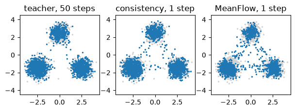
def renoised_sample(u, z, key):
    """Two evaluations of a one-time map: jump, re-noise to t = 0.5, jump."""
    x = d2l.flow_map_sample(u, z, 1)
    half = jnp.full((len(z),), 0.5)
    return d2l.flow_map_sample(u, lin.sample(x, half, jax.random.normal(
        key, x.shape)), 1, t_start=0.5)

cm, mf = students['consistency'], students['MeanFlow']
samples = {'data': mix.sample(jax.random.key(3), 20_000),
           'teacher, 50 steps': d2l.flow_map_sample(
               lambda x, s, t: teacher(x, t), z, 50),
           'consistency, 1': d2l.flow_map_sample(cm, z, 1),
           'consistency, 2 re-noised': renoised_sample(cm, z,
                                                       jax.random.key(4)),
           **{f'MeanFlow, {k}': d2l.flow_map_sample(mf, z, k)
              for k in (1, 2, 4)}}
for name, x in samples.items():
    s = mix.summary(x)
    print(f'{name:>24}: weights {s["weights"]}, stray {s["stray"]:.1%}, '
          f'spread {s["spread"]:.3f}')
d2l.scatter_panels([samples[k][:2000] for k in
                    ('teacher, 50 steps', 'consistency, 1', 'MeanFlow, 1')],
                   ['teacher, 50 steps', 'consistency, 1 step',
                    'MeanFlow, 1 step'],
                   data=mix.sample(jax.random.key(5), 2000), size=2.4);
data: weights [0.496, 0.3, 0.203], stray 1.1%, spread 0.474
teacher, 50 steps: weights [0.499, 0.298, 0.203], stray 1.5%, spread 0.463
consistency, 1: weights [0.497, 0.299, 0.205], stray 2.0%, spread 0.458
consistency, 2 re-noised: weights [0.496, 0.298, 0.205], stray 1.2%, spread 0.478
MeanFlow, 1: weights [0.505, 0.296, 0.198], stray 4.1%, spread 0.331
MeanFlow, 2: weights [0.503, 0.296, 0.201], stray 1.3%, spread 0.386
MeanFlow, 4: weights [0.501, 0.298, 0.202], stray 0.7%, spread 0.371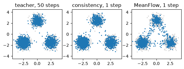
Both students reproduce the mixture in one evaluation, with weights within about 0.015 of 0.5/0.3/0.2. The fresh draw strays about 1.1% of the time, the tail of each Gaussian beyond three standard deviations, and the teacher with fifty Euler steps about 1.5%. The consistency student strays about 2% after one evaluation. The MeanFlow student, trained without a teacher, strays about 4%, and its other samples sit closer to the mode centers than the data do. A second evaluation, re-noised or a second jump, brings the strays of both to the teacher’s level. MeanFlow’s samples stay too tight, though: their spread is about 0.38 after two and four jumps against 0.47 for the data, which is also why four jumps stray less often than the data themselves.
MeanFlow’s ImageNet recipe divides each example’s squared error \(e\) by \((e + c)^p\), held fixed, with \(p = 1\) and a small \(c\), so that the gradient is that of \(\log(e + c)\). Squared error is minimized by the conditional mean of the target, its logarithm near the most probable value. Without a teacher the targets at a noisy point spread over the three modes, so the weighted loss should pull the field toward the heaviest mode. We train the MeanFlow student again with this weight.
def weighted_meanflow_loss(u, x0, c=1e-3):
    """The MeanFlow loss with each squared error e divided by e + c, fixed."""
    a, b = torch.rand(2, len(x0), device=device)
    e = d2l.flow_map_error(u, None, x0, torch.randn_like(x0),
                           torch.minimum(a, b), torch.maximum(a, b))
    return (e / (e.detach() + c)).mean()

torch.manual_seed(2)
_, weighted, _ = d2l.train_regression(
    MLPFlowMap(256, 3, num_times=2).to(device), weighted_meanflow_loss,
    lambda: mix.sample(512), 20_000, cosine=True)
s = mix.summary(d2l.flow_map_sample(weighted, z, 1))
print(f'weighted MeanFlow, 1: weights {s["weights"]}, stray {s["stray"]:.1%}')
weighted MeanFlow, 1: weights [0.944, 0.027, 0.029], stray 2.3%def weighted_meanflow_loss(u, x0, key, c=1e-3):
"""The MeanFlow loss with each squared error e divided by e + c, fixed."""
k1, k2 = jax.random.split(key)
a, b = jax.random.uniform(k1, (2, len(x0)))
e = d2l.flow_map_error(u, None, x0, jax.random.normal(k2, x0.shape),
jnp.minimum(a, b), jnp.maximum(a, b))
return (e / (jax.lax.stop_gradient(e) + c)).mean()
_, weighted, _ = d2l.train_regression(
MLPFlowMap(256, 3, num_times=2, rngs=nnx.Rngs(2)), weighted_meanflow_loss,
lambda k: mix.sample(k, 512), 20_000, jax.random.key(2), cosine=True)
s = mix.summary(d2l.flow_map_sample(weighted, z, 1))
print(f'weighted MeanFlow, 1: weights {s["weights"]}, stray {s["stray"]:.1%}')weighted MeanFlow, 1: weights [0.945, 0.039, 0.016], stray 1.8%The weighted student puts more than nine samples in ten on the heaviest mode, and few of them stray: the loss has fitted the most probable target instead of the average one. Plain squared error recovers the weights, which is why the other losses take the plain mean of flow_map_error.
17.7.3.2 On Images
On Fashion-MNIST we distil the unconditional U-Net of Section 17.4, about 1.2 million parameters trained for 10,000 updates, through the moving average of its weights. We train it again here.
X, y, X_test, y_test = d2l.load_fashion_mnist_pm1()

def batch_fn():
    return X[torch.randint(0, len(X), (128,), device=X.device)]

torch.manual_seed(0)
_, teacher, _ = d2l.train_regression(d2l.UNet(ch=64).to(X.device),
                                     d2l.regression_loss(lin, 'velocity'),
                                     batch_fn, 10_000)
X, y, X_test, y_test = d2l.load_fashion_mnist_pm1()
def batch_fn(key):
return X[jax.random.randint(key, (128,), 0, len(X))]
_, teacher, _ = d2l.train_regression(d2l.UNet(ch=64, rngs=nnx.Rngs(0)),
d2l.regression_loss(lin, 'velocity'),
batch_fn, 10_000, jax.random.key(0))We score 1,000 samples by the Fréchet distance (FD) of Section 17.3 against 1,000 test images, read against the floor of two disjoint sets of 1,000 test images.
cnn = d2l.fashion_feature_cnn(X, y)
features = lambda imgs: d2l.fd_features(cnn, imgs)
f_test = features(X_test[:1000])
floor = d2l.fid_score(features(X_test[1000:2000]), f_test)
print(f'floor, 1,000 real images against 1,000 others: FD {floor:.2f}')
floor, 1,000 real images against 1,000 others: FD 0.80cnn = d2l.fashion_feature_cnn(X, y)
features = lambda imgs: d2l.fd_features(cnn, imgs)
f_test = features(X_test[:1000])
floor = d2l.fid_score(features(X_test[1000:2000]), f_test)
print(f'floor, 1,000 real images against 1,000 others: FD {floor:.2f}')floor, 1,000 real images against 1,000 others: FD 0.83The student is UNetFlowMap on the teacher’s averaged weights, trained with the teacher’s velocity and both times free. Half of the pairs have \(s = t\), where the loss is the teacher’s own velocity loss; the other half draw \(s < t\) as on the mixture. Starting from trained weights, it learns at a rate of \(2 \cdot 10^{-4}\) for 5,000 updates, half the teacher’s 10,000.
def student_loss(u, x0):
    a, b = torch.rand(2, len(x0), device=x0.device)
    s, t = torch.minimum(a, b), torch.maximum(a, b)
    # half the pairs have s = t: the plain flow-matching term
    s = torch.where(torch.rand(len(x0), device=x0.device) < 0.5, t, s)
    return d2l.flow_map_error(u, teacher, x0, torch.randn_like(x0), s,
                              t).mean()

torch.manual_seed(2)
_, student, _ = d2l.train_regression(  # jvp through GroupNorm won't compile
    d2l.UNetFlowMap(teacher).to(X.device), student_loss, batch_fn, 5_000,
    lr=2e-4, ema_half_life=500, compiled=False)
def student_loss(u, x0, key):
k1, k2, k3 = jax.random.split(key, 3)
a, b = jax.random.uniform(k1, (2, len(x0)))
s, t = jnp.minimum(a, b), jnp.maximum(a, b)
# half the pairs have s = t: the plain flow-matching term
s = jnp.where(jax.random.uniform(k2, (len(x0),)) < 0.5, t, s)
return d2l.flow_map_error(u, teacher, x0, jax.random.normal(k3, x0.shape),
s, t).mean()
_, student, _ = d2l.train_regression(
d2l.UNetFlowMap(teacher, rngs=nnx.Rngs(2)), student_loss, batch_fn,
5_000, jax.random.key(2), lr=2e-4, ema_half_life=500)From the same 1,000 noise images, the teacher takes 1 to 50 Euler steps and the student 1, 2 or 4 jumps, and we plot FD against the number of network evaluations.
torch.manual_seed(3)
noise = torch.randn(1000, 1, 28, 28, device=X.device)
velocity = lambda x, s, t: teacher(x, t)
ns_teacher, ns_student = (1, 2, 4, 10, 20, 50), (1, 2, 4)
images = {('teacher', n): d2l.flow_map_sample(velocity, noise, n)
          for n in ns_teacher}
images |= {('student', n): d2l.flow_map_sample(student, noise, n)
           for n in ns_student}
fd = {key: d2l.fid_score(features(x), f_test) for key, x in images.items()}
for (name, n), v in fd.items():
    print(f'{name}, {n:2d} evaluations: FD {v:6.2f}')
d2l.plot([ns_teacher, ns_student, [1, 50]],
         [[fd['teacher', n] for n in ns_teacher],
          [fd['student', n] for n in ns_student], [floor, floor]],
         'network evaluations', 'FD',
         legend=['teacher, Euler', 'student, jumps', 'floor'],
         xscale='log', yscale='log', fmts=('o-', 's-', 'k:'))
teacher, 1 evaluations: FD 167.10
teacher, 2 evaluations: FD 82.75
teacher, 4 evaluations: FD 26.93
teacher, 10 evaluations: FD 6.62
teacher, 20 evaluations: FD 3.56
teacher, 50 evaluations: FD 2.55
student, 1 evaluations: FD 11.70
student, 2 evaluations: FD 4.68
student, 4 evaluations: FD 3.46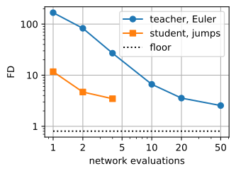
noise = jax.random.normal(jax.random.key(3), (1000, 28, 28, 1))
velocity = lambda x, s, t: teacher(x, t)
ns_teacher, ns_student = (1, 2, 4, 10, 20, 50), (1, 2, 4)
images = {('teacher', n): d2l.flow_map_sample(velocity, noise, n)
          for n in ns_teacher}
images |= {('student', n): d2l.flow_map_sample(student, noise, n)
           for n in ns_student}
fd = {key: d2l.fid_score(features(x), f_test) for key, x in images.items()}
for (name, n), v in fd.items():
    print(f'{name}, {n:2d} evaluations: FD {v:6.2f}')
d2l.plot([ns_teacher, ns_student, [1, 50]],
         [[fd['teacher', n] for n in ns_teacher],
          [fd['student', n] for n in ns_student], [floor, floor]],
         'network evaluations', 'FD',
         legend=['teacher, Euler', 'student, jumps', 'floor'],
         xscale='log', yscale='log', fmts=('o-', 's-', 'k:'))
teacher, 1 evaluations: FD 141.68
teacher, 2 evaluations: FD 73.83
teacher, 4 evaluations: FD 26.12
teacher, 10 evaluations: FD 6.99
teacher, 20 evaluations: FD 4.07
teacher, 50 evaluations: FD 2.80
student, 1 evaluations: FD 11.50
student, 2 evaluations: FD 5.41
student, 4 evaluations: FD 3.83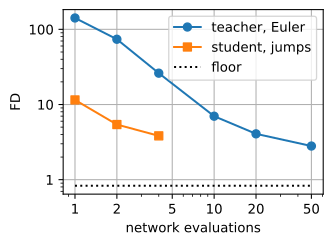
The teacher’s FD falls from about 150 at one Euler step and 70 to 85 at two to about 7 at ten and 2.5 to 2.8 at fifty, against a floor of about 0.8. The student lies far below this curve at small budgets: one jump scores about 4 to 5 times the teacher’s fifty-step FD, two jumps about twice, and four within about 1.5 times. Two evaluations of the student are worth about fifteen Euler steps of the teacher, and one about seven.
The remaining gap at one evaluation is a matter of budget. The students in the papers train for roughly 100,000 to 800,000 iterations at batches of 512, two to three orders of magnitude more than ours, and report one-step FIDs about 1.4 to 1.7 times those of their teachers. Training our student longer lowers its one-step FD only slowly.
The rows below are drawn from the same eight noise images: the teacher with fifty and with two Euler steps, and the student with one and with two jumps.
rows = [('teacher', 50), ('teacher', 2), ('student', 1), ('student', 2)]
d2l.show_gray(torch.cat([images[r][:8].clamp(-1, 1) for r in rows]), 4, 8);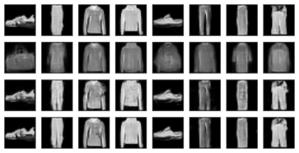
rows = [('teacher', 50), ('teacher', 2), ('student', 1), ('student', 2)]
d2l.show_gray(jnp.concatenate([images[r][:8].clip(-1, 1) for r in rows]),
              4, 8);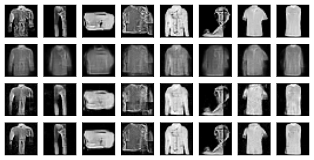
The rows match column by column. Two Euler steps of the teacher draw grey averages of garments, the collapse of the first section in pixels. The student draws the teacher’s garment from each noise image, sharp but over-contrasted and sometimes broken after one jump and close to the teacher’s after two.
17.7.4 The Other Route: Matching Distributions
A flow map regresses onto a target computed from an ODE’s trajectories, so its student can be no better than those trajectories. The distillation methods of Section 16.7 instead train a one-step generator to match the distribution of the data, with a critic against real images (Sauer et al. 2023) or with the difference between the teacher’s score and that of the student’s own samples (Yin et al. 2024). Both give up the bijection, so inversion and editing through the ODE no longer apply. They gain quality in one step, and with real images in the loss a student can surpass its teacher (Section 16.8).
Classifier-free guidance (Section 17.3) evaluates the network twice per step. Meng et al. (2023) distil the guided velocity into one network that takes the guidance strength as an input, which halves the cost of every step before the number of steps is reduced (Exercise 8).
17.7.5 Summary
One Euler step from noise lands on the mean of the data, and straightening the field reduces the number of steps but not to one. A flow map learns where a trajectory arrives instead of where it points. Differentiating its definition along the trajectory gives the MeanFlow identity, a regression target that needs one Jacobian-vector product and either a teacher’s velocity or each example’s conditional velocity; with \(s = 0\) and a teacher it is consistency distillation. On the mixture one evaluation recovers the mode weights; on images a short student comes within about 1.5 times the teacher’s FD in four evaluations. All of this needs a continuous path and a velocity, which do not exist when \(\mathbf{x}\) is a sequence of tokens, the subject of Section 17.8.
17.7.6 Exercises
- One and two Euler steps.
- A single step of the deterministic sampler from pure noise to \(t = 0\) returns \(\mathbb{E}[\mathbf{x}_0]\) from every start, whatever the path (Section 17.2). Does the same hold for one Euler step in \(t\), \(\mathbf{x} - \mathbf{u}_1(\mathbf{x})\), on the cosine path \(\alpha_t = \cos\frac{\pi t}{2}\), \(\sigma_t = \sin\frac{\pi t}{2}\)? What does that step return, and why does an Euler step in \(t\) depend on the path when a step in \(\bar\sigma\) does not?
- Let the data be the two points \(\pm a\) in one dimension, with equal probability, on the linear path. Show that \(\mathbb{E}[x_0 \mid x_t = x] = a \tanh\big(a (1 - t) x / t^2\big)\) and that two Euler steps of length \(\tfrac12\) map a start \(x\) to \(a \tanh(a x)\). Section 43.6.1.3 has the exact flow of this example.
- For \(a = 2\), what fraction of the two-step samples lies within \(0.1\) of a data point? Where does the exact flow map \(\Phi_{1 \to 0}\) send \(x\)?
- [code] Reflow on the mixture. ● Reflow (Liu et al. 2023) retrains a velocity model on pairs of a noise vector and the sample that the current model produces from it.
- Draw 20,000 noise vectors, integrate the teacher of this section with fifty Euler steps, and train a new
TimeMLPon the pairs with the velocity loss and the teacher’s settings. - Report the weights and strays of the new model at 1, 2, 4 and 10 Euler steps, and the mean distance of its fifty-step trajectories from their chords, next to the same quantities for the teacher.
- Which of the teacher’s errors does reflow remove, which does it inherit, and which does it add? What would a second round do to each?
- Draw 20,000 noise vectors, integrate the teacher of this section with fifty Euler steps, and train a new
- [code] Progressive distillation. ● Salimans and Ho (2022) train a student so that one of its steps reproduces two steps of the teacher, then make the student the teacher and repeat.
- On the mixture, start from 64 Euler steps of the teacher of this section and halve the number of steps six times, training each student for a fifth of the teacher’s updates. Which identity of the flow map does each round enforce?
- Report the strays after each round, and compare the one-step student with the flow-map students of this section at equal total training steps. Where do the errors of the rounds come from?
- [code] Which time pairs to train on. The MeanFlow student drew every pair with \(s < t\), the image student half of them with \(s = t\).
- Train the MeanFlow student on the mixture with a share of \(0.25\), \(0.5\), \(0.75\) and \(1\) of the pairs having \(s < t\), and report the strays at one and two jumps. Which share serves one jump best?
- Replace the uniform times by a logit-normal distribution of \(t\) with mean \(-0.4\) and standard deviation \(1\), which concentrates the times in the middle of the path. What changes, and why?
- Why might pairs with \(s = t\) matter more on images, where the student starts from the teacher’s weights, than on the mixture, where it starts from random weights?
- [code] The derivative against a difference. ● Consistency distillation as published (Song et al. 2023) uses a grid of \(N = 18\) times, one Heun step of the teacher from \(t_n\) to \(t_{n-1}\), and a target held fixed at the earlier point.
- Write the student as \(f(\mathbf{x}, t) = \mathbf{x} - t\, \bar{\mathbf{u}}(\mathbf{x}, 0, t)\) and show that the difference of its outputs at the two points, divided by \(t_n - t_{n-1}\), tends to the Eulerian derivative Equation 17.7.2 at \(s = 0\) as \(N\) grows.
- Implement the discrete loss without a Jacobian-vector product, train it on the mixture with the teacher of this section, and compare its one-step strays with those of the continuous student. Try \(N = 8\) and \(N = 64\). Does a finer grid help, and why?
- [code] The stop-gradient. Copy
flow_map_errorinto a cell and remove the stop-gradient on the target.- Train the MeanFlow student on the mixture with this loss and report its one-step weights and strays. Write out the gradient of the loss with the target differentiated, and identify the term that the stop-gradient removes. What can the network change to lower this loss without satisfying Equation 17.7.3?
- Song et al. compute the target with a moving average of the student’s weights instead. Implement this with
d2l.EMAand compare.
- The Lagrangian loss. ● Boffi et al. (2025) train flow maps with the Lagrangian identity.
- Substitute Equation 17.7.1 into \(\partial_s \Phi_{t \to s}(\mathbf{x}) = \mathbf{u}_s(\Phi_{t \to s}(\mathbf{x}))\) and derive an identity for \(\bar{\mathbf{u}}\) that involves the velocity at the output of the jump.
- Why can the conditional velocity \(\boldsymbol\epsilon - \mathbf{x}_0\) not serve in this identity, so that a velocity model is needed? Show that the flow map’s own velocity \(\bar{\mathbf{u}}(\cdot, s, s)\) can serve, so that one network trains itself.
- [code] Train such a student on the mixture and compare it with the MeanFlow student in strays and in training cost per step.
- [code] A guided student. ● Train the class-conditional U-Net of Section 17.3 and distil it into a two-time student whose reference velocity \(\mathbf{u}_{\textrm{ref}}\) is the guided velocity \(\tilde{\mathbf{u}}\),
d2l.cfg(teacher, c, 2.0), for random labels \(c\), with the label as an input of the student.- Compare the FD and the agreement of the predicted class with the requested one for the teacher with fifty guided Euler steps and the student with one, two and four jumps.
- How many network evaluations does each sample cost in each case?
- [code] Quality against cost. Measure the wall-clock time per 1,000 images and the FD of the teacher of this section with 1 to 50 Euler steps, with Heun’s method on the crowded grid of Section 17.4, and of the student with 1 to 4 jumps.
- Plot FD against time. At which FD do the curves cross?
- The student cost extra training. How many images must be generated before that training is repaid at the FD of two jumps?
- Matching noised distributions. ● Score-difference distillation (Yin et al. 2024) trains a one-step generator \(\mathbf{x} = g_{\boldsymbol\theta}(\mathbf{z})\) along \(\mathbb{E}\big[(\nabla \log q_{\boldsymbol\theta, t}(\mathbf{x}_t) - \nabla \log p_t(\mathbf{x}_t))^\top \partial \mathbf{x}_t / \partial \boldsymbol\theta\big]\), where \(\mathbf{x}_t = \alpha_t g_{\boldsymbol\theta}(\mathbf{z}) + \sigma_t \boldsymbol\epsilon\) and \(q_{\boldsymbol\theta, t}\) is the law of \(\mathbf{x}_t\): the score of its own noised samples minus the teacher’s.
- Show that this is the gradient of \(D_{\textrm{KL}}(q_{\boldsymbol\theta, t} \,\|\, p_t)\). Why does the term from the dependence of \(q_{\boldsymbol\theta, t}\) itself on \(\boldsymbol\theta\) vanish?
- In one dimension, let the generator be \(m + s z\) with \(s > 0\) and the data \(\mathcal{N}(\mu, v)\). Write \(D_{\textrm{KL}}(q_t \,\|\, p_t)\) on the linear path in closed form, and show that \(m = \mu\), \(s^2 = v\) is its only minimizer at every \(t < 1\).
- Let the data be \(\tfrac12 \mathcal{N}(-2, 0.25) + \tfrac12 \mathcal{N}(2, 0.25)\). Evaluate \(D_{\textrm{KL}}(q_t \,\|\, p_t)\) by quadrature on a grid of \((m, s)\) at \(t \in \{0.1, 0.3, 0.5, 0.9\}\), and locate the minimizer at each \(t\). Why is the minimum near \(\log 2\) at small \(t\)? Relate the result to mode dropping in GANs (Section 16.1.3.3) and to the merging of modes under noise (6). What does a weighting of the levels toward large \(t\) buy a Gaussian generator, and what can no weighting buy it?
- [extended] Shortcut models. ●● A shortcut model (Frans et al. 2025) conditions a velocity model on the step size \(d\) and trains it from scratch with two losses: flow matching at \(d = 0\), and self-consistency, which asks one step of size \(2d\) to equal two steps of size \(d\) computed by the model itself and held fixed.
- Which identity of the flow map does self-consistency enforce, and why does it need no Jacobian-vector product?
- Implement it on the mixture with step sizes \(2^{-k}\), \(k = 0, \ldots, 6\), and compare its strays at one, two and four steps with those of the MeanFlow student at equal training steps.