%matplotlib inline
from d2l import torch as d2l
import time
import torch
from torch import nn
from torch.nn import functional as F11.1 The Transformer Block
The previous chapter developed attention as a layer in which each position can read from the others. Deployed models place this layer in a transformer block. Attention communicates between positions, a position-wise feed-forward network transforms each position independently, and both add their outputs to a shared residual stream. This section studies two design choices that distinguish the original block from current ones: the placement of normalization and the form of the feed-forward network. Experiments examine signal propagation at initialization and compare a standard MLP with its gated successor at matched parameter count. We then combine these choices in a configurable TransformerBlock class used throughout the remainder of the chapter.
%matplotlib inline
from d2l import jax as d2l
from flax import nnx
import jax
from jax import numpy as jnp
import optax
import time
11.1.1 Components of a Transformer Block
A transformer block contains two sublayers connected by a residual stream. Section 10.6 introduced the residual stream view: each token carries a running vector \(\mathbf{x} \in \mathbb{R}^d\) from layer to layer, and sublayers do not replace it — they read from it, compute, and add their result back. The block’s two sublayers divide the labor:
- Attention is the only place where positions interact. Each token queries the others as in Section 10.3 and adds the retrieved mixture to its stream. Contextual information enters through this sublayer.
- The feed-forward network (FFN) acts on each position separately: the same two- or three-matrix MLP is applied token by token, with no interaction between positions. It transforms each token’s accumulated state and contains most of the block’s parameters.
Writing \(\mathrm{Attn}\) for multi-head self-attention and \(\mathrm{Norm}\) for a normalization layer, the modern (pre-norm) block computes
\[ \mathbf{h} = \mathbf{x} + \mathrm{Attn}(\mathrm{Norm}_1(\mathbf{x})), \qquad \mathbf{y} = \mathbf{h} + \mathrm{FFN}(\mathrm{Norm}_2(\mathbf{h})). \tag{11.1.1}\]
Both sublayers preserve the shape \((n, d)\): the block maps a sequence of \(d\)-dimensional vectors to a sequence of the same length and width, which is what makes stacking dozens of copies possible. Note also what the block does not contain: positions. Attention is permutation equivariant (Section 10.4), and the block does nothing to change that — positional information is the model’s job, not the block’s, a division of responsibilities the next section exploits.
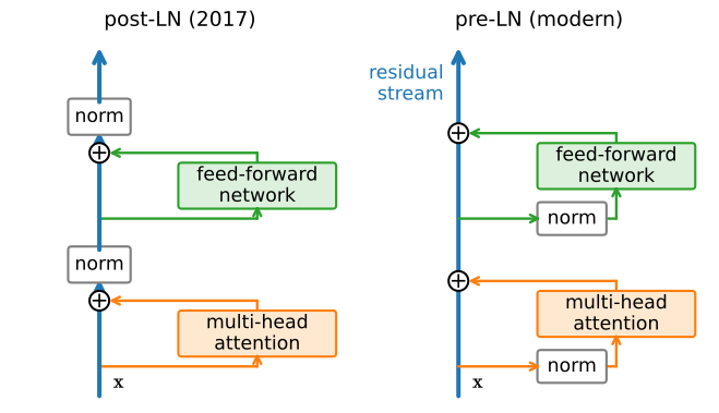
Figure 11.1.1 shows the wiring, in the two normalization arrangements compared below.
11.1.2 Where the Normalization Goes
Residual connections and normalization entered the block together in 2017 (Vaswani et al. 2017): without some control on scale, the sum of dozens of sublayer outputs drifts, and training deep stacks becomes a tuning nightmare. The normalizer of choice is layer normalization (Ba et al. 2016), which standardizes each token’s vector across its \(d\) features — unlike the batch normalization of Section 7.3, it involves no batch statistics, so it behaves identically in training and inference and is indifferent to sequence length. The 2017 paper also fixed where it goes, and a few years of painful experience revised that answer.
11.1.2.1 Two Arrangements
The original block normalizes the stream after each addition (“post-LN”):
\[ \mathbf{h} = \mathrm{Norm}_1(\mathbf{x} + \mathrm{Attn}(\mathbf{x})), \qquad \mathbf{y} = \mathrm{Norm}_2(\mathbf{h} + \mathrm{FFN}(\mathbf{h})). \tag{11.1.2}\]
The modern block Equation 11.1.1 normalizes each branch’s input (“pre-LN”) and leaves the stream alone. In code the two differ by two lines. The minimal block below takes the arrangement as a flag; its attention is the d2l.MultiHeadAttention of Section 10.3 and its FFN is the classic two-matrix MLP (we upgrade both ingredients later in this section).
class MiniBlock(nn.Module):
    """Attention + MLP on a residual stream; norm placement as a flag."""
    def __init__(self, num_hiddens, pre_norm):
        super().__init__()
        self.pre_norm = pre_norm
        self.attention = d2l.MultiHeadAttention(num_hiddens, 4, dropout=0)
        self.W_1 = nn.Linear(num_hiddens, 4 * num_hiddens)
        self.W_2 = nn.Linear(4 * num_hiddens, num_hiddens)
        self.norm1 = nn.LayerNorm(num_hiddens)
        self.norm2 = nn.LayerNorm(num_hiddens)

    def ffn(self, X):
        return self.W_2(F.gelu(self.W_1(X)))

    def forward(self, X):
        if self.pre_norm:
            Y = self.norm1(X)
            X = X + self.attention(Y, Y, Y, None)
            return X + self.ffn(self.norm2(X))
        X = self.norm1(X + self.attention(X, X, X, None))
        return self.norm2(X + self.ffn(X))
class MiniBlock(nnx.Module):
"""Attention + MLP on a residual stream; norm placement as a flag."""
def __init__(self, num_hiddens, pre_norm, rngs=None):
rngs = nnx.Rngs(0) if rngs is None else rngs
self.pre_norm = pre_norm
self.attention = d2l.MultiHeadAttention(num_hiddens, 4, dropout=0,
rngs=rngs)
self.W_1 = nnx.Linear(num_hiddens, 4 * num_hiddens, rngs=rngs)
self.W_2 = nnx.Linear(4 * num_hiddens, num_hiddens, rngs=rngs)
self.norm1 = nnx.LayerNorm(num_hiddens, rngs=rngs)
self.norm2 = nnx.LayerNorm(num_hiddens, rngs=rngs)
def ffn(self, X):
return self.W_2(nnx.gelu(self.W_1(X)))
def __call__(self, X):
if self.pre_norm:
Y = self.norm1(X)
X = X + self.attention(Y, Y, Y, None)[0]
return X + self.ffn(self.norm2(X))
X = self.norm1(X + self.attention(X, X, X, None)[0])
return self.norm2(X + self.ffn(X))11.1.2.2 Signal Propagation at Initialization
Which arrangement is better? We can get a long way without training anything. A freshly initialized network is a fixed random function, so we can measure how it treats signals. We stack \(N\) blocks, pass a random sequence through them, and measure the output without training. Fixing the seed makes the experiment deterministic. We initialize every weight matrix as the original transformer did (Xavier initialization) and track three quantities: the scale of the residual stream, how distinct the tokens remain from one another, and how much gradient each block’s attention receives from a generic loss at the top.
For the distinctness measure we use the cross-token spread \(\|\mathbf{H} - \bar{\mathbf{H}}\| / \|\mathbf{H}\|\), where \(\bar{\mathbf{H}}\) copies the average token to every position: it is \(1\) when tokens are unrelated and \(0\) when they have collapsed onto a single point. One caution learned the hard way: after a final normalization layer the naive probe loss \(\|\mathbf{H}\|^2\) is constant by construction, so we probe with a generic linear readout \(\langle \mathbf{R}, \mathbf{H} \rangle\) for fixed random \(\mathbf{R}\) instead.
def signal_stats(pre_norm, num_blks=32, num_hiddens=256):
    torch.manual_seed(0)
    blks = nn.ModuleList([MiniBlock(num_hiddens, pre_norm)
                          for _ in range(num_blks)])
    torch.manual_seed(1)
    X = torch.randn(2, 64, num_hiddens)
    H = X
    for blk in blks:
        H = blk(H)                      # materialize the lazy layers
    for p in blks.parameters():
        if p.ndim == 2:                 # the 2017 initialization
            nn.init.xavier_uniform_(p)
    H, spreads, rms = X, [], []
    for blk in blks:
        H = blk(H)
        spreads.append(
            ((H - H.mean(1, keepdim=True)).norm() / H.norm()).item())
        rms.append(H.pow(2).mean().sqrt().item())
    (H * torch.randn_like(H)).mean().backward()  # generic readout loss
    grads = [blk.attention.W_q.weight.grad.norm().item() for blk in blks]
    proj = {n: getattr(blks[-1].attention, n).weight.grad.norm().item()
            for n in ('W_q', 'W_k', 'W_v', 'W_o')}
    return spreads, rms, grads, proj

stats = {pre: signal_stats(pre) for pre in (False, True)}
for pre, name in ((False, 'post-LN'), (True, 'pre-LN')):
    spreads, rms, grads, proj = stats[pre]
    print(f'{name:>8}: stream RMS at k=32: {rms[-1]:5.2f},  '
          'token spread at k=8,16,32: '
          + ' '.join(f'{spreads[k-1]:8.1e}' for k in (8, 16, 32)))
    print('          grad norms at k=32: '
          + '  '.join(f'{n} {g:7.1e}' for n, g in proj.items()))
d2l.plot(torch.arange(1, 33), [stats[False][2], stats[True][2]],
         'block index k', 'query projection gradient norm',
         legend=['post-LN', 'pre-LN'], yscale='log')
post-LN: stream RMS at k=32: 1.00, token spread at k=8,16,32: 3.7e-01 3.6e-02 1.2e-04
grad norms at k=32: W_q 2.9e-09 W_k 2.6e-09 W_v 5.8e-02 W_o 5.9e-02
pre-LN: stream RMS at k=32: 5.25, token spread at k=8,16,32: 7.4e-01 5.2e-01 3.7e-01
grad norms at k=32: W_q 1.9e-03 W_k 1.9e-03 W_v 8.1e-02 W_o 8.4e-02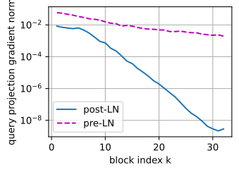
class Stack(nnx.Module):
    def __init__(self, num_blks, pre_norm, num_hiddens=256, rngs=None):
        rngs = nnx.Rngs(0) if rngs is None else rngs
        self.blks = nnx.List([MiniBlock(num_hiddens, pre_norm, rngs)
                              for _ in range(num_blks)])

    def __call__(self, X):
        for blk in self.blks:
            X = blk(X)
        return X

def signal_stats(pre_norm, num_blks=32, num_hiddens=256):
    stack = Stack(num_blks, pre_norm, num_hiddens, rngs=nnx.Rngs(0))
    init, key = nnx.initializers.xavier_uniform(), jax.random.key(0)
    flat = []
    for path, p in nnx.to_flat_state(nnx.state(stack, nnx.Param)):
        if p[...].ndim == 2:           # the 2017 initialization
            key, sub = jax.random.split(key)
            p = jax.tree.map(lambda v: init(sub, v.shape), p)
        flat.append((path, p))
    nnx.update(stack, nnx.from_flat_state(flat))
    X = jax.random.normal(jax.random.key(1), (2, 64, num_hiddens))
    R = jax.random.normal(jax.random.key(2), (2, 64, num_hiddens))
    H, spreads, rms = X, [], []
    for blk in stack.blks:
        H = blk(H)
        spreads.append(float(jnp.linalg.norm(H - H.mean(1, keepdims=True))
                             / jnp.linalg.norm(H)))
        rms.append(float(jnp.sqrt((H ** 2).mean())))
    grads = nnx.grad(lambda m: (m(X) * R).mean())(stack)  # generic readout
    top = grads['blks'][num_blks - 1]['attention']
    proj = {n: float(jnp.linalg.norm(top[n]['kernel'][...]))
            for n in ('W_q', 'W_k', 'W_v', 'W_o')}
    grads = [float(jnp.linalg.norm(
        grads['blks'][k]['attention']['W_q']['kernel'][...]))
        for k in range(num_blks)]
    return spreads, rms, grads, proj

stats = {pre: signal_stats(pre) for pre in (False, True)}
for pre, name in ((False, 'post-LN'), (True, 'pre-LN')):
    spreads, rms, grads, proj = stats[pre]
    print(f'{name:>8}: stream RMS at k=32: {rms[-1]:5.2f},  '
          'token spread at k=8,16,32: '
          + ' '.join(f'{spreads[k-1]:8.1e}' for k in (8, 16, 32)))
    print('          grad norms at k=32: '
          + '  '.join(f'{n} {g:7.1e}' for n, g in proj.items()))
d2l.plot(jnp.arange(1, 33), [stats[False][2], stats[True][2]],
         'block index k', 'query projection gradient norm',
         legend=['post-LN', 'pre-LN'], yscale='log')
post-LN: stream RMS at k=32: 1.00, token spread at k=8,16,32: 3.5e-01 2.5e-02 2.0e-04
grad norms at k=32: W_q 5.6e-09 W_k 4.9e-09 W_v 6.5e-02 W_o 6.6e-02
pre-LN: stream RMS at k=32: 5.22, token spread at k=8,16,32: 7.2e-01 5.3e-01 3.7e-01
grad norms at k=32: W_q 2.3e-03 W_k 2.3e-03 W_v 8.2e-02 W_o 8.4e-02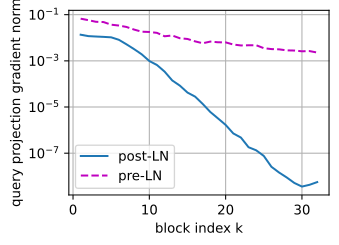
The two arrangements produce different networks at the same parameter values. Post-LN renormalizes the stream after every addition, so its RMS is pinned at \(1\) at every depth; pre-LN only ever adds, so its stream grows like the square root of the depth (the block outputs are nearly independent at initialization, and variances add). That growth is not a defect — it is a protection. Each pre-LN branch reads the stream through its own normalization, so as the stream grows, each successive block’s relative contribution shrinks, and the function stays tame.
The post-LN stack has no such damping, and the token-spread column shows what happens instead. At initialization attention is nearly uniform, so every attention sublayer pulls each token toward the average token; post-LN then renormalizes, locking in the contraction, and the spread decays geometrically — by block 32 the tokens are identical to about one part in ten thousand. Pre-LN dilutes the same contraction by the growing stream, and the spread falls only polynomially, still at \(0.4\) after 32 blocks. The decreasing token spread is an initialization-time diagnostic related to the rank-collapse phenomenon analyzed by Dong et al. (2021); it does not demonstrate collapse during training. In this 32-block stack, the post-LN query and key projections receive gradients of order \(10^{-9}\), about six orders of magnitude below their pre-LN counterparts, while the value and output projection norms are near \(0.06\). Once token representations become nearly identical, the attention mixture becomes insensitive to the query and key weights, which explains the small gradients in this constructed setting. Different initializations, residual scales, optimizers, and training dynamics can change the effect (Xiong et al. 2020).
The experiments of Xiong et al. (2020) likewise find that post-LN is more sensitive to learning-rate warmup than pre-LN under their training protocols. We therefore use pre-norm as the default in the teaching model and test both placements during training in Section 11.2.
11.1.2.3 RMSNorm
Modern models also simplified the normalizer itself. LayerNorm standardizes each token vector by subtracting its mean and dividing by its standard deviation, then rescales (and re-shifts) feature-wise. RMSNorm (Zhang and Sennrich 2019) drops the centering and the shift, keeping only the part that controls scale:
\[ \mathrm{RMSNorm}(\mathbf{x}) = \frac{\mathbf{x}}{\sqrt{\tfrac{1}{d} \sum_{i=1}^{d} x_i^2 + \epsilon}} \odot \boldsymbol{\gamma}. \tag{11.1.3}\]
It is a one-line function, and both frameworks ship it; let’s verify our implementation against the built-in and time the two normalizers.
def rms_norm(X, weight, eps=1e-6):
    return X / torch.sqrt((X * X).mean(-1, keepdim=True) + eps) * weight

device = d2l.try_gpu()
X = torch.randn(64, 512, 1024, device=device)
layernorm = nn.LayerNorm(1024, device=device)
rmsnorm = nn.RMSNorm(1024, eps=1e-6, device=device)
print(f'ours vs. built-in: max deviation '
      f'{(rms_norm(X, rmsnorm.weight) - rmsnorm(X)).abs().max():.1e}')
for name, f in (('LayerNorm', layernorm), ('RMSNorm', rmsnorm)):
    for _ in range(10):
        f(X)                       # warmup
    if device.type == 'cuda':
        torch.cuda.synchronize()
    t0 = time.time()
    for _ in range(200):
        f(X)
    if device.type == 'cuda':
        torch.cuda.synchronize()
    print(f'{name}: {(time.time() - t0) / 200 * 1e3:.3f} ms')
ours vs. built-in: max deviation 9.5e-07
LayerNorm: 0.681 ms
RMSNorm: 0.652 msdef rms_norm(X, weight, eps=1e-6):
return X / jnp.sqrt((X * X).mean(-1, keepdims=True) + eps) * weight
X = jax.random.normal(jax.random.key(0), (64, 512, 1024))
layernorm = nnx.LayerNorm(1024, rngs=nnx.Rngs(0))
rmsnorm = nnx.RMSNorm(1024, epsilon=1e-6, rngs=nnx.Rngs(0))
print(f'ours vs. built-in: max deviation '
f'{jnp.abs(rms_norm(X, rmsnorm.scale[...]) - rmsnorm(X)).max():.1e}')
for name, f in (('LayerNorm', nnx.jit(layernorm)),
('RMSNorm', nnx.jit(rmsnorm))):
f(X).block_until_ready() # warmup + compile
t0 = time.time()
for _ in range(200):
Y = f(X)
Y.block_until_ready()
print(f'{name}: {(time.time() - t0) / 200 * 1e3:.3f} ms')ours vs. built-in: max deviation 9.5e-07
LayerNorm: 1.076 ms
RMSNorm: 0.732 msIn this benchmark, the PyTorch timings are indistinguishable at the displayed precision, while the JAX RMSNorm kernel is roughly one third faster. These are framework- and device-specific measurements rather than an architectural speed guarantee. RMSNorm omits centering and a bias parameter and computes one statistic instead of two; its quality must be assessed in the surrounding model. Llama is one prominent model family that uses it (Touvron et al. 2023a).
11.1.2.4 Normalizing Queries and Keys
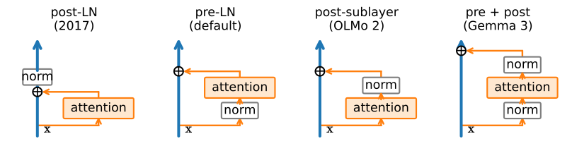
One more normalization migrated inside attention. Nothing in the block above controls the size of the attention logits \(\mathbf{q}^\top \mathbf{k} / \sqrt{d}\) themselves: if training inflates the queries and keys, the softmax saturates, its Jacobian vanishes (Section 10.2), and training can spike or stall — an instability first met at vision-transformer scale, where attention entropy was observed collapsing in billion-parameter runs (Dehghani et al. 2023). QK-norm (Henry et al. 2020) applies RMSNorm to the queries and keys per head, right before the dot product, thereby controlling vector norms before scoring. It costs two extra norms per layer. Reports for Gemma 3, Qwen3, and OLMo 2 document its use in those model families. OLMo 2 combines QK-norm with normalization after each sublayer but outside the residual stream’s identity path (Team OLMo et al. 2025); Gemma 3 normalizes each branch both before and after the sublayer (Gemma Team 2025). Figure 11.1.2 compares these placements. Only original post-LN normalizes the residual stream after addition; the signal experiment above directly compares that arrangement with pre-LN. We leave QK-norm as an exercise rather than a flag; it drops into the block through the attn_factory hook introduced below.
11.1.3 The Feed-Forward Network
Between the attention sublayers sits the block’s other half: a small MLP applied to each position independently,
\[ \mathrm{FFN}(\mathbf{x}) = \mathbf{W}_2\, \phi(\mathbf{W}_1 \mathbf{x}), \tag{11.1.4}\]
with \(\mathbf{W}_1 \in \mathbb{R}^{4d \times d}\) and \(\mathbf{W}_2 \in \mathbb{R}^{d \times 4d}\) in the classic configuration. The factor-4 expansion is a convention the field has never found strong reason to revisit, and it implies something worth noticing: the FFN holds \(8d^2\) parameters against attention’s \(4d^2\), so about two thirds of a block’s parameters sit in these two matrices. When people say a transformer’s knowledge lives mostly in its FFNs, this ratio is the accounting behind the claim.
Two upgrades separate the 2017 FFN from today’s. The activation \(\phi\) moved from ReLU to GELU (Hendrycks and Gimpel 2016), a smoothed relative that ends the debate about the kink at zero (GPT onward (Radford et al. 2018)). Then Shazeer (2020) revived an older idea — gating — and found that a gated linear unit with the SiLU activation beat both:
\[ \mathrm{SwiGLU}(\mathbf{x}) = \mathbf{W}_2 \big(\mathrm{SiLU}(\mathbf{W}_g \mathbf{x}) \odot \mathbf{W}_1 \mathbf{x}\big), \qquad \mathrm{SiLU}(z) = z \cdot \mathrm{sigmoid}(z). \tag{11.1.5}\]
Instead of gating a linear transform through a fixed nonlinearity, SwiGLU computes two linear views of the input and multiplies them, one squashed into a soft gate, the other passed through untouched — the value is transmitted at full strength wherever the gate is open, rather than bent through the activation. The multiplicative interaction is the same trick gates played in LSTMs, here compressed into a single layer. A third matrix means more parameters at the same width, so fair comparisons shrink the hidden width to \(\tfrac{8}{3} d\), making the three matrices of the gated FFN cost the same \(8d^2\) as the classic one, up to rounding. Both variants, in one class:
class FeedForward(nn.Module):
    """Position-wise FFN: GELU MLP or SwiGLU at matched parameter count."""
    def __init__(self, num_hiddens, act='swiglu', bias=False):
        super().__init__()
        assert act in ('swiglu', 'gelu'), f'unknown act: {act!r}'
        self.act = act
        if act == 'gelu':
            width = 4 * num_hiddens
        else:  # 'swiglu': three matrices; width 8d/3 matches the MLP budget
            width = round(8 * num_hiddens / 3)
            self.W_g = nn.Linear(num_hiddens, width, bias=bias)
        self.W_1 = nn.Linear(num_hiddens, width, bias=bias)
        self.W_2 = nn.Linear(width, num_hiddens, bias=bias)

    def forward(self, X):
        if self.act == 'gelu':
            return self.W_2(F.gelu(self.W_1(X), approximate='tanh'))
        return self.W_2(F.silu(self.W_g(X)) * self.W_1(X))
class FeedForward(nnx.Module):
"""Position-wise FFN: GELU MLP or SwiGLU at matched parameter count."""
def __init__(self, num_hiddens, act='swiglu', bias=False, rngs=None):
rngs = nnx.Rngs(0) if rngs is None else rngs
assert act in ('swiglu', 'gelu'), f'unknown act: {act!r}'
self.act = act
if act == 'gelu':
width = 4 * num_hiddens
else: # 'swiglu': three matrices; width 8d/3 matches the MLP budget
width = round(8 * num_hiddens / 3)
self.W_g = nnx.Linear(num_hiddens, width, use_bias=bias,
rngs=rngs)
self.W_1 = nnx.Linear(num_hiddens, width, use_bias=bias, rngs=rngs)
self.W_2 = nnx.Linear(width, num_hiddens, use_bias=bias, rngs=rngs)
def __call__(self, X):
if self.act == 'gelu':
return self.W_2(nnx.gelu(self.W_1(X)))
return self.W_2(nnx.silu(self.W_g(X)) * self.W_1(X))(The GELU here is the tanh approximation, the exact variant GPT-2 shipped with — a detail that will matter when we load its weights in Section 11.2.) The parameter match is worth checking rather than trusting:
for act in ('gelu', 'swiglu'):
    ffn = FeedForward(256, act)
    print(f'{act:>7}: {sum(p.numel() for p in ffn.parameters())} parameters')
gelu: 524288 parameters
swiglu: 524544 parametersfor act in ('gelu', 'swiglu'):
ffn = FeedForward(256, act)
n = sum(p.size for p in jax.tree.leaves(nnx.state(ffn, nnx.Param)))
print(f'{act:>7}: {n} parameters') gelu: 524288 parameters
swiglu: 524544 parametersWhether the gate improves performance at equal parameter count is an empirical question. The final experiment compares the alternatives in a small language model.
11.1.4 A Configurable Block
We assemble the block used throughout this chapter. Every design decision above becomes a constructor argument. norm selects LayerNorm or RMSNorm, act selects the FFN, pre_norm selects the arrangement, and two factory hooks let later sections swap whole sublayers — a mixture-of-experts FFN, or a cache-friendly grouped-query attention — without touching this class again. The constructor validates its flag strings: a typo must fail loudly, not silently select an architecture. The default configuration (pre-norm, RMSNorm, SwiGLU) is the one you would find inside an open-weights model released this year; TransformerBlock(num_hiddens, num_heads, norm='layer', act='gelu', pre_norm=False, bias=True) is a compact post-norm block in the 2017 encoder arrangement (with one anachronism kept for simplicity: GELU, where the 2017 original used ReLU).
class TransformerBlock(nn.Module):
    """Configurable transformer block: attention + FFN on a residual
    stream."""
    def __init__(self, num_hiddens, num_heads, dropout=0, norm='rms',
                 act='swiglu', pre_norm=True, bias=False, attn_factory=None,
                 ffn_factory=None):
        super().__init__()
        assert norm in ('rms', 'layer'), f'unknown norm: {norm!r}'
        assert num_hiddens % num_heads == 0
        self.pre_norm = pre_norm
        make_norm = nn.RMSNorm if norm == 'rms' else nn.LayerNorm
        self.norm1, self.norm2 = make_norm(num_hiddens), make_norm(num_hiddens)
        self.attention = (d2l.MultiHeadAttention(num_hiddens, num_heads,
                                                 dropout, bias=bias)
                          if attn_factory is None else attn_factory())
        self.ffn = (FeedForward(num_hiddens, act, bias=bias)
                    if ffn_factory is None else ffn_factory())
        self.dropout = nn.Dropout(dropout)

    def forward(self, X, valid_lens=None):
        if self.pre_norm:
            Y = self.norm1(X)
            X = X + self.dropout(self.attention(Y, Y, Y, valid_lens))
            return X + self.dropout(self.ffn(self.norm2(X)))
        X = self.norm1(X + self.dropout(self.attention(X, X, X, valid_lens)))
        return self.norm2(X + self.dropout(self.ffn(X)))
class TransformerBlock(nnx.Module):
"""Configurable transformer block: attention + FFN on a residual
stream."""
def __init__(self, num_hiddens, num_heads, dropout=0, norm='rms',
act='swiglu', pre_norm=True, bias=False, attn_factory=None,
ffn_factory=None, rngs=None):
rngs = nnx.Rngs(params=0, dropout=1) if rngs is None else rngs
assert norm in ('rms', 'layer'), f'unknown norm: {norm!r}'
assert num_hiddens % num_heads == 0
self.pre_norm = pre_norm
make_norm = nnx.RMSNorm if norm == 'rms' else nnx.LayerNorm
self.norm1 = make_norm(num_hiddens, rngs=rngs)
self.norm2 = make_norm(num_hiddens, rngs=rngs)
self.attention = (d2l.MultiHeadAttention(num_hiddens, num_heads,
dropout, bias=bias,
rngs=rngs)
if attn_factory is None else attn_factory(rngs))
self.ffn = (FeedForward(num_hiddens, act, bias=bias, rngs=rngs)
if ffn_factory is None else ffn_factory(rngs))
self.dropout = nnx.Dropout(dropout, rngs=rngs)
def __call__(self, X, valid_lens=None):
if self.pre_norm:
Y = self.norm1(X)
X = X + self.dropout(self.attention(Y, Y, Y, valid_lens)[0])
return X + self.dropout(self.ffn(self.norm2(X)))
X = self.norm1(X + self.dropout(
self.attention(X, X, X, valid_lens)[0]))
return self.norm2(X + self.dropout(self.ffn(X)))11.1.4.1 Shapes and Parameters
The block preserves its input shape whatever the flags, and its parameter census confirms the accounting from above: \(4d^2\) in attention, \(8d^2\) in the FFN (however the activation slices it), and a rounding error of normalization weights — about \(12d^2\) per block, two thirds of it FFN.
X = torch.ones(2, 10, 256)
blk = TransformerBlock(256, num_heads=8)
blk2017 = TransformerBlock(256, num_heads=8, norm='layer', act='gelu',
                           pre_norm=False, bias=True)
d2l.check_shape(blk(X), X.shape)
d2l.check_shape(blk2017(X), X.shape)
count = lambda m: sum(p.numel() for p in m.parameters())
print(f'attention {count(blk.attention)}, ffn {count(blk.ffn)}, '
      f'total {count(blk)} = {count(blk) / 256 ** 2:.2f} d^2')
attention 262144, ffn 524544, total 787200 = 12.01 d^2X = jnp.ones((2, 10, 256))
blk = TransformerBlock(256, num_heads=8)
blk2017 = TransformerBlock(256, num_heads=8, norm='layer', act='gelu',
pre_norm=False, bias=True)
d2l.check_shape(blk(X), X.shape)
d2l.check_shape(blk2017(X), X.shape)
count = lambda m: sum(p.size for p in jax.tree.leaves(
nnx.state(m, nnx.Param)))
print(f'attention {count(blk.attention)}, ffn {count(blk.ffn)}, '
f'total {count(blk)} = {count(blk) / 256 ** 2:.2f} d^2')attention 262144, ffn 524544, total 787200 = 12.01 d^2One block is not yet a language model, but it is close enough to train. The same valid_lens mechanism that masked padding in Section 10.2 makes the block causal: pass each query a valid length equal to its own position, and every token attends only backward. A dozen lines wrap an embedding, a stack of blocks, and a tied output head (as in Section 10.4) around that trick:
class CharLM(nn.Module):
    """Minimal char LM: causal masking via per-query valid lengths."""
    def __init__(self, vocab_size, num_hiddens=128, num_heads=4, num_blks=2,
                 act='swiglu', max_len=128):
        super().__init__()
        self.token_emb = nn.Embedding(vocab_size, num_hiddens)
        self.pos_emb = nn.Embedding(max_len, num_hiddens)
        for emb in (self.token_emb, self.pos_emb):
            nn.init.normal_(emb.weight, std=0.02)
        self.blks = nn.ModuleList([
            TransformerBlock(num_hiddens, num_heads, act=act)
            for _ in range(num_blks)])
        self.norm = nn.RMSNorm(num_hiddens)

    def forward(self, X):
        B, T = X.shape
        H = self.token_emb(X) + self.pos_emb(
            torch.arange(T, device=X.device))
        causal = torch.arange(1, T + 1, device=X.device).repeat(B, 1)
        for blk in self.blks:
            H = blk(H, causal)
        return F.linear(self.norm(H), self.token_emb.weight)
class CharLM(nnx.Module):
"""Minimal char LM: causal masking via per-query valid lengths."""
def __init__(self, vocab_size, num_hiddens=128, num_heads=4, num_blks=2,
act='swiglu', max_len=128, rngs=None):
rngs = nnx.Rngs(0) if rngs is None else rngs
init = nnx.initializers.normal(0.02)
self.token_emb = nnx.Embed(vocab_size, num_hiddens,
embedding_init=init, rngs=rngs)
self.pos_emb = nnx.Embed(max_len, num_hiddens,
embedding_init=init, rngs=rngs)
self.blks = nnx.List([
TransformerBlock(num_hiddens, num_heads, act=act, rngs=rngs)
for _ in range(num_blks)])
self.norm = nnx.RMSNorm(num_hiddens, rngs=rngs)
def __call__(self, X):
B, T = X.shape
H = self.token_emb(X) + self.pos_emb(jnp.arange(T))
causal = jnp.tile(jnp.arange(1, T + 1), (B, 1))
for blk in self.blks:
H = blk(H, causal)
return self.token_emb.attend(self.norm(H))11.1.4.2 Comparing GELU and SwiGLU
We compare the two alternatives on the same data (the character-level Time Machine corpus of Section 8.2), holding the model, seed, optimizer, learning rate, and 600-step budget fixed. Only the act flag differs, and the parameter counts match to a tenth of a percent.
data = d2l.TimeMachine(batch_size=64, num_steps=128, tokenization='char',
                       num_train=100000, num_val=3000)
for act in ('gelu', 'swiglu'):
    torch.manual_seed(0)
    model = CharLM(len(data.vocab), act=act)
    losses = d2l.train_lm(model, data,
                          torch.optim.AdamW(model.parameters(), lr=1e-3,
                                            weight_decay=0.0), 600)
    print(f'{act:>7}: loss at step 200/400/600: ' + '/'.join(
        f'{sum(losses[k-100:k]) / 100:.2f}' for k in (200, 400, 600)))
gelu: loss at step 200/400/600: 2.26/1.65/1.31
swiglu: loss at step 200/400/600: 2.24/1.51/1.17data = d2l.TimeMachine(batch_size=64, num_steps=128, tokenization='char',
num_train=100000, num_val=3000)
for act in ('gelu', 'swiglu'):
model = CharLM(len(data.vocab), act=act, rngs=nnx.Rngs(0))
optimizer = nnx.Optimizer(model, optax.adamw(1e-3, weight_decay=0.0),
wrt=nnx.Param)
losses = d2l.train_lm(model, data, optimizer, 600)
print(f'{act:>7}: loss at step 200/400/600: ' + '/'.join(
f'{sum(losses[k-100:k]) / 100:.2f}' for k in (200, 400, 600))) gelu: loss at step 200/400/600: 2.27/1.73/1.41
swiglu: loss at step 200/400/600: 2.22/1.57/1.24The gated FFN ends more than a tenth of a nat ahead. This margin holds up across seeds, since rerunning with seeds 1 and 2 moves each number by a couple of hundredths, not the gap. More importantly, it agrees in direction with Shazeer (2020)’s systematic sweep and with the consistent choice of the major model families since Llama. It is a modest, real improvement at equal parameter count. Such incremental gains can accumulate when several architectural choices are combined.
The diagnostics in this section use one initialization, a 32-block synthetic stack, and framework-specific normalization kernels. They establish algebraic identities and report local signal, gradient, timing, and loss measurements; they do not by themselves establish causal explanations or universal model rankings. The cited large-scale studies provide separate evidence for the training practices discussed above.
11.1.5 Summary
A transformer block contains attention and a position-wise FFN connected through a residual stream. Attention communicates between positions; the FFN transforms each position and contains about two thirds of the parameters. In the original post-LN arrangement, normalization fixes the scale of the residual stream, but the query and key projections near the top of a 32-block stack receive gradients six orders of magnitude smaller than those near the bottom. Pre-norm instead normalizes each branch input and preserves usable gradients throughout the stack. RMSNorm retains only the scale statistic, while QK-norm controls the scale of attention logits. Finally, SwiGLU replaces a fixed activation with a learned gate and gives a small, seed-stable improvement at matched parameter count in our experiment. The resulting TransformerBlock exposes normalization, activation, and placement as options, with replaceable attention and FFN modules.
11.1.6 Exercises
- Scale invariance. Let RMSNorm act as in Equation 11.1.3 with \(\boldsymbol{\gamma} = \mathbf{1}\) and \(\epsilon = 0\), and write \(r(\mathbf{x}) = (\tfrac{1}{d} \sum_i x_i^2)^{1/2}\) for the root mean square of \(\mathbf{x} \in \mathbb{R}^d\).
- Show that \(\mathrm{RMSNorm}(\alpha \mathbf{x}) = \mathrm{RMSNorm}(\mathbf{x})\) for every \(\alpha > 0\), and that LayerNorm with unit gain and zero shift is also unchanged when the same constant is added to every coordinate. Describe the set of inputs that each normalizer maps to a given output.
- Show that the Jacobian of RMSNorm at \(\mathbf{x}\) is \(r(\mathbf{x})^{-1} (\mathbf{I} - \hat{\mathbf{x}} \hat{\mathbf{x}}^\top)\) with \(\hat{\mathbf{x}} = \mathbf{x} / \|\mathbf{x}\|\). Conclude that the gradient \(\nabla_{\mathbf{x}} \ell\) is orthogonal to \(\mathbf{x}\) for every loss \(\ell\) that depends on \(\mathbf{x}\) only through \(\mathrm{RMSNorm}(\mathbf{x})\).
- Scale-invariant weights. ● Let the loss be invariant to the scale of a parameter matrix, \(\ell(\alpha \mathbf{W}) = \ell(\mathbf{W})\) for all \(\alpha > 0\). Under QK-norm with \(\epsilon = 0\) and without a query bias, this holds for the rows of \(\mathbf{W}_q\) that produce the queries of one head.
- Show that \(\langle \mathbf{W}, \nabla_{\mathbf{W}} \ell \rangle = 0\) and that a gradient-descent step never decreases \(\|\mathbf{W}\|_F\).
- Show that the gradient at \(\alpha \mathbf{W}\) is \(\alpha^{-1}\) times the gradient at \(\mathbf{W}\). Explain how the angle through which one step turns \(\mathbf{W}\) changes as its norm grows during training.
- Unrolled residual stream. Number the \(2N\) sublayers of an \(N\)-block stack by \(j = 1, \ldots, 2N\), write \(F_j\) for the \(j\)-th sublayer (attention or FFN) and \(\mathrm{Norm}_j\) for its normalization, and let \(\mathbf{x}_j\) be the residual stream after sublayer \(j\), so that \(\mathbf{x}_0\) is the input.
- For the pre-LN arrangement Equation 11.1.1, write \(\mathbf{x}_{2N}\) as \(\mathbf{x}_0\) plus a sum of \(2N\) branch outputs. Write the Jacobian \(\partial \mathbf{x}_{2N} / \partial \mathbf{x}_0\) as a product over sublayers, expand the product, and identify the term that passes a gradient from the output to the input unchanged.
- For the post-LN arrangement Equation 11.1.2, the stream is \(\mathbf{x}_j = \mathrm{Norm}_j(\mathbf{u}_j)\) with \(\mathbf{u}_j = \mathbf{x}_{j-1} + F_j(\mathbf{x}_{j-1})\). Model every normalization as RMSNorm with unit gain and \(\epsilon = 0\). Assume that the input \(\mathbf{x}_0\) has unit root mean square and that each branch output is uncorrelated with the stream it is added to. The product of the normalization Jacobians alone takes the place of the identity term of the pre-LN expansion. Show that this product scales a vector orthogonal to every \(\mathbf{u}_j\) by \(\prod_j r(\mathbf{u}_j)^{-1}\), and write this factor as a function of the mean squares \(c_1, \ldots, c_{2N}\) of the branch outputs. Evaluate it for a common mean square \(c_j = c\), and compare its dependence on \(N\) with that of the identity term of the pre-LN expansion.
CharLMapplies a final RMSNorm,norm, before its tied output head. Describe what the head would receive without it as a pre-LN stack grows deeper, and explain why a post-LN stack needs no final normalization.
- [code] Stream variance budget. ● In the pre-LN arrangement every branch reads a normalized input. If each branch output is uncorrelated with the stream it is added to, the mean square of the stream after \(k\) blocks is \[1 + \sum_{i=1}^{k} \big(c^\textrm{attn}_i + c^\textrm{ffn}_i\big),\] where \(c^\textrm{attn}_i\) and \(c^\textrm{ffn}_i\) are the mean squares of the attention and FFN outputs of block \(i\). Use
MiniBlockwith the Xavier initialization ofsignal_statsat \(d = 256\).- Predict \(c^\textrm{ffn}_1\). Compute the variance of the hidden pre-activations of the FFN, and evaluate the second moment of GELU at that variance numerically.
- Predict \(c^\textrm{attn}_1\). Treat the \(n = 64\) input tokens as independent, and treat the attention logits of one query as independent Gaussians with the variance that the initialization implies.
- Record the mean square of each branch output in
signal_statsand plot \(c^\textrm{attn}_k\) and \(c^\textrm{ffn}_k\) against \(k\). Compare block 1 with your predictions, and explain the trend of \(c^\textrm{attn}_k\) using the token spread. - Fit a power law to the stream RMS, once over blocks 1 to 32 and once over blocks 8 to 32. Compare both exponents with \(1/2\), explain the comparison with the variance budget, and state the regime in which the square-root growth stated in Section 11.1.2.2 holds.
- [code] Rate of token collapse. ● Write the tokens of one sequence as \(\mathbf{x}_i = \boldsymbol{\mu} + \boldsymbol{\delta}_i\) for \(i = 1, \ldots, n\), where \(\boldsymbol{\mu}\) is the mean token and \(\sum_i \boldsymbol{\delta}_i = \mathbf{0}\). With the ratio of common to deviation energy \[\rho = \frac{n \|\boldsymbol{\mu}\|^2}{\sum_i \|\boldsymbol{\delta}_i\|^2}, \tag{11.1.6}\] the token spread of
signal_statsequals \((1 + \rho)^{-1/2}\). At initialization the attention weights are nearly uniform, so a post-LN attention sublayer adds approximately the same vector \(\mathbf{W}_o \mathbf{W}_v \boldsymbol{\mu}\) to every token, where \(\mathbf{W}_v, \mathbf{W}_o \in \mathbb{R}^{d \times d}\) are the value and output projections.- Let the entries of \(\mathbf{W}_v\) and \(\mathbf{W}_o\) be independent with mean zero and variance \(\alpha^2 / d\), so that \(\alpha = 1\) is Xavier initialization of a square matrix. Treat the normalization as a rescaling common to all tokens. Show that one attention sublayer and its normalization multiply \(\rho\) by about \(1 + \alpha^4\), and derive the spread after \(k\) blocks for an input of \(n\) independent random tokens, ignoring the FFN sublayers.
- Rerun
signal_statsfor post-LN with all Xavier weights multiplied by \(\alpha \in \{1, 0.7, 0.5\}\), once with the fullMiniBlockand once with its FFN sublayer removed. Compare both with your formula at blocks 8, 16, and 32, and explain the remaining gap of the full block. - GPT-1 stacked 12 post-LN blocks of width \(d = 768\) and drew every weight from \(\mathcal{N}(0, 0.02^2)\) (Radford et al. 2018). Compute \(\alpha\) for its attention projections, and predict the spread after 12 blocks for \(n = 64\), both for this initialization and for Xavier initialization at the same width. Check both predictions with
signal_stats.
- [code] QK-norm as a factory. QK-norm
(Section 11.1.2.4) applies RMSNorm over the head dimension \(p = d/h\) to every query and key just before the scores are computed.
- Write
QKNormAttention, a subclass ofd2l.MultiHeadAttentionin which the queries and the keys returned bytranspose_qkveach pass through their own RMSNorm before the dot product. Build aTransformerBlockwith it throughattn_factoryand check the output shape. - Show that with unit gains every scaled logit \(\hat{\mathbf{q}}^\top \hat{\mathbf{k}} / \sqrt{p}\) lies in \([-\sqrt{p}, \sqrt{p}]\), and generalize the bound to learned gains \(\boldsymbol{\gamma}_q\) and \(\boldsymbol{\gamma}_k\). Compute the largest possible ratio between two attention weights of one query for \(p = 64\) and unit gains.
- Training can inflate the query and key weights. Mimic this at initialization: multiply the weights of
W_qandW_kof a freshly initialized layer with \(d = 256\) and \(h = 4\) by \(\lambda \in \{1, 2, 4, 8\}\), and feed it 64 standard normal tokens. Measure the standard deviation of the logits and the mean entropy of the attention weights, with and without QK-norm. Compare the entropies with \(\log 64\), and explain the shape of each curve.
- Write
- [code] Off-stream normalization. ● OLMo 2 normalizes the output of each branch instead of its input (Team OLMo et al. 2025), \[\mathbf{h} = \mathbf{x} + \mathrm{Norm}(\mathrm{Attn}(\mathbf{x})), \tag{11.1.7}\] and Gemma 3 normalizes both the input and the output of each branch (Gemma Team 2025), \[\mathbf{h} = \mathbf{x} + \mathrm{Norm}'(\mathrm{Attn}(\mathrm{Norm}(\mathbf{x}))), \tag{11.1.8}\] with the FFN sublayer treated identically in both. Figure 11.1.2 draws these two placements next to post-LN and pre-LN.
- Predict the stream RMS after \(N\) blocks at initialization for both arrangements.
- Replace the
pre_normflag ofMiniBlockby a string that selects one of the four arrangements, and extendsignal_statsto record the mean entropy of the attention weights of each block. Compare the stream RMS, the token spread, the query-projection gradient norms, and the entropies of all four arrangements. - Explain the entropies that you measure in the upper blocks of the OLMo 2 stack, and name the failure that takes the place of the token collapse of post-LN.
- Replace the attention of the OLMo 2 arrangement and of the post-LN arrangement by
QKNormAttentionand rerun the experiment. Compare the effect of QK-norm on the entropies and the token spread of both arrangements, and relate each effect to the cause of that arrangement’s failure.
- FFN width rounding.
FeedForwardsets the SwiGLU width to \(\mathrm{round}(8d/3)\).- Write the exact parameter count of the default
TransformerBlock(d, h)as a function of \(d\), and bound the relative deviation of its FFN from \(8d^2\). - The released 7B configuration of Llama (Touvron et al. 2023a) has \(d = 4096\) and SwiGLU width \(11008\), the smallest multiple of 256 that is at least \(\lfloor 8d/3 \rfloor\). Compute the relative excess of its FFN parameters over \(8d^2\), and the excess that the same rule gives at \(d = 256\) and at \(d = 128\), the default
num_hiddensofCharLM. Explain what the comparison implies for parameter-matched experiments with small models.
- Write the exact parameter count of the default
- [code] Normalization cost. A kernel is memory-bound when moving its data between memory and the processor takes longer than its arithmetic, so that its runtime is close to the number of bytes moved divided by the memory bandwidth.
- Recreate the tensor
Xof Section 11.1.2.3, of shape \((64, 512, 1024)\) in 32-bit floats. Count the bytes that LayerNorm and RMSNorm must at least read and write, and the floating-point operations per element of each. - Time the elementwise map \(\mathbf{X} \mapsto 2\mathbf{X}\) in the same way as the two normalizers, and convert all three timings into achieved bandwidths in GB/s.
- Use the achieved bandwidths to estimate how many passes over
Xeach normalizer makes. Explain why dropping the centering and one statistic need not change the runtime of a normalizer that readsXonce, and describe an implementation in which RMSNorm would be measurably faster.
- Recreate the tensor
- [code] Gated variants. Shazeer (2020) varies the gate of
Equation 11.1.5. ReGLU replaces SiLU by ReLU, GEGLU replaces it by GELU, and the bilinear variant drops the activation and multiplies the two linear views \(\mathbf{W}_g \mathbf{x}\) and \(\mathbf{W}_1
\mathbf{x}\) directly.
- Extend
FeedForwardwith these three settings ofactat width \(\mathrm{round}(8d/3)\), and check that all gated settings have the same parameter count. - Train
CharLMwith each of the five settings for three seeds under the protocol of Section 11.1.4.2. Report the mean and the standard deviation over seeds of the loss averaged over the last 100 steps. - Compare your ranking with Table 1 of Shazeer (2020) . Compare the gap between the bilinear variant and the GELU MLP with the spread among the four gated variants, and state which ingredient of SwiGLU the comparison credits with its improvement.
- Extend
- [extended] Learning-rate sensitivity. ● Wortsman et al. (2024) reproduce the growth of attention logits reported for large training runs (Section 11.1.2.4) in small models trained at high learning rates, and find that QK-norm removes it. They summarize the final loss \(\ell(\eta)\) as a function of the learning rate \(\eta\) by the learning-rate sensitivity \[\mathbb{E}_{\eta}\big[\min(\ell(\eta), \ell_0) - \ell^*\big], \tag{11.1.9}\] where \(\ell_0\) is the loss at initialization, \(\ell^*\) is the best final loss over the learning rates tried, and the average runs over learning rates spanning three orders of magnitude.
- Give
CharLMan option that builds its blocks withQKNormAttentionthroughattn_factory. Withnum_hiddens=256andnum_blks=6, train it with and without QK-norm for 1000 steps at each learning rate in \(\{10^{-4}, 10^{-3.5}, \ldots, 10^{-1}\}\), otherwise under the protocol of Section 11.1.4.2. - Every 100 steps, record the training loss and the largest absolute attention logit on a fixed batch. Plot the final loss against \(\eta\) for both models, and compute the learning-rate sensitivity of each curve.
- For every learning rate at which the model without QK-norm ends worse than the model with it, decide from the recorded attention logits whether attention-logit growth explains the gap. If it does not, record the largest absolute output logit of both models at the same steps, and decide whether its growth explains the gap.
- Give