%matplotlib inline
from d2l import torch as d2l
import math
import torch
from torch import nn12.1 Gated Recurrence
Section 8.6.2.1 showed that the gradient that travels \(k\) steps back through a vanilla RNN is multiplied by the \(k\)-th power of the recurrent Jacobian, so it shrinks or grows geometrically. Gradient clipping limits growth but does not recover a vanished signal. This motivates changing the recurrence through multiplicative gating, a mechanism that lets the network learn what to write into its memory, what to erase, and what to reveal. The analysis behind it goes back to Hochreiter’s 1991 diploma thesis and to Bengio et al. (1994) (see also (Hochreiter et al. 2001)), and its most famous product is the long short-term memory (LSTM) cell of Hochreiter and Schmidhuber (1997), which powered speech recognition, translation, and language modeling for most of the 2010s.
Gating also appears in newer architectures. The transformer’s gated feed-forward networks multiply one branch of activations by another, a design whose value Section 11.1 measured directly, and modern linear recurrences use an input-dependent forgetting coefficient around a linear state. We first develop the gate, then implement the LSTM from scratch and with framework layers. The gated recurrent unit (GRU) follows as a streamlined descendant. We conclude with two structural axes, depth and bidirectionality, and a survey of current uses of gating.
Prerequisites: the RNN language-modeling pipeline of Section 8.5 (data, scaffold, and training recipe are reused verbatim) and the gradient analysis of Section 8.6.2.1.
%matplotlib inline
from d2l import jax as d2l
from flax import nnx
import jax
from jax import numpy as jnp
import math
12.1.1 Controlling Memory Updates
Start from what the gradient analysis demands. As motivation, take the simplest caricature: if the state-to-state Jacobian were one fixed matrix, the contribution of a dependency \(k\) steps back would scale asymptotically as \(\rho^k\), where \(\rho\) is the spectral radius, and the only value of \(\rho\) that neither buries nor explodes distant information is \(1\). (The full story is subtler — a product of time-varying, generally non-normal Jacobians can grow for many steps even with every eigenvalue inside the unit circle, a phenomenon Section 24.2.2 develops — but the caricature points at the right target.) The simplest recurrence with that property is an accumulator,
\[ \mathbf{S}_t = \mathbf{S}_{t-1} + (\textrm{new content}), \tag{12.1.1}\]
whose Jacobian \(\partial \mathbf{S}_t / \partial \mathbf{S}_{t-1}\) is exactly the identity: gradients pass backwards through it unattenuated, no matter how many steps they travel. Additive updates, not repeated matrix multiplication, are the memory-friendly primitive.
But a pure accumulator cannot discard obsolete information. Every update remains in the sum, so irrelevant inputs interfere with relevant ones and the state magnitude typically grows with sequence length. A useful memory must make decisions. Should this input be written down? Should this stored value be kept or cleared? Should the memory influence the output right now, or stay silent? What turns these discrete-sounding decisions into something a network can learn is the gate: a small sigmoid-activated layer of the current input and the previous state,
\[ \mathbf{G}_t = \sigma(\mathbf{X}_t \mathbf{W}_{\textrm{xg}} + \mathbf{H}_{t-1} \mathbf{W}_{\textrm{hg}} + \mathbf{b}_\textrm{g}), \tag{12.1.2}\]
whose entries lie in \((0, 1)\) and multiply a signal elementwise. A gate value near \(1\) lets its coordinate pass; a value near \(0\) blocks it; values in between attenuate. Because the gate is computed from context, the decision is different at every time step and for every unit, and because \(\sigma\) is smooth, the decision is differentiable and trainable by the same backpropagation used for the other parameters. Every architecture in this section is a particular arrangement of a few such gates around an additive state.
The gate provides a direct response to the stability question in Section 8.6.2.1. A vanilla RNN has one shared matrix \(\mathbf{W}_{\textrm{hh}}\) whose spectrum governs every perturbation in every direction at every step. Preserving gradients requires training to keep this global matrix near \(\rho = 1\). In a gated cell, the state coordinate \(i\) is scaled by the gate value \(g_{t,i} \in (0, 1)\) at step \(t\), so a perturbation from \(k\) steps ago is scaled by the product \(\prod_{j} g_{j,i} \leq 1\): growth is impossible along the memory path, while holding the gate near \(1\) makes the product, and hence the preserved memory, as close to lossless as the task requires. In dynamical-systems terms, each unit gets its own learned, input-dependent rate of decay in place of one hard-wired global one. Some units learn to forget in three steps; others hold a value across an entire sequence.
12.1.2 Long Short-Term Memory
12.1.2.1 The Memory Cell and Its Gates
The LSTM replaces the vanilla RNN’s hidden node with a memory cell. The name “long short-term memory” describes its role: a network’s weights are its long-term memory, changing slowly across training, while its activations are short-term memory, overwritten at every step; the cell is an intermediate store, an activation engineered to persist. Concretely, the cell keeps an internal state \(\mathbf{C}_t\), the additive accumulator of the previous section, and controls it with three gates computed exactly in the form of Equation 12.1.2. With a minibatch of \(n\) examples, \(d\)-dimensional inputs \(\mathbf{X}_t \in \mathbb{R}^{n \times d}\), and \(h\) hidden units carrying the previous state \(\mathbf{H}_{t-1} \in \mathbb{R}^{n \times h}\), the input gate \(\mathbf{I}_t\), forget gate \(\mathbf{F}_t\), and output gate \(\mathbf{O}_t\), each in \(\mathbb{R}^{n \times h}\), are
\[ \begin{aligned} \mathbf{I}_t &= \sigma(\mathbf{X}_t \mathbf{W}_{\textrm{xi}} + \mathbf{H}_{t-1} \mathbf{W}_{\textrm{hi}} + \mathbf{b}_\textrm{i}),\\ \mathbf{F}_t &= \sigma(\mathbf{X}_t \mathbf{W}_{\textrm{xf}} + \mathbf{H}_{t-1} \mathbf{W}_{\textrm{hf}} + \mathbf{b}_\textrm{f}),\\ \mathbf{O}_t &= \sigma(\mathbf{X}_t \mathbf{W}_{\textrm{xo}} + \mathbf{H}_{t-1} \mathbf{W}_{\textrm{ho}} + \mathbf{b}_\textrm{o}), \end{aligned} \tag{12.1.3}\]
where the \(\mathbf{W}_{\textrm{x}\cdot} \in \mathbb{R}^{d \times h}\) and \(\mathbf{W}_{\textrm{h}\cdot} \in \mathbb{R}^{h \times h}\) are weights and the \(\mathbf{b}_\cdot \in \mathbb{R}^{1 \times h}\) are biases (broadcast over the batch as in Section 1.1.4). A fourth head, the input node, proposes the content that might be written. It uses \(\tanh\) rather than \(\sigma\), since content should be able to be negative:
\[ \tilde{\mathbf{C}}_t = \tanh(\mathbf{X}_t \mathbf{W}_{\textrm{xc}} + \mathbf{H}_{t-1} \mathbf{W}_{\textrm{hc}} + \mathbf{b}_\textrm{c}). \tag{12.1.4}\]
The four heads are the same computation with different nonlinearities and different jobs. What distinguishes the LSTM is how they combine. The forget gate scales the old cell state, the input gate scales the proposed content, and the two are added; the output gate then decides how much of the (squashed) cell is exposed as the hidden state:
\[ \mathbf{C}_t = \mathbf{F}_t \odot \mathbf{C}_{t-1} + \mathbf{I}_t \odot \tilde{\mathbf{C}}_t, \qquad \mathbf{H}_t = \mathbf{O}_t \odot \tanh(\mathbf{C}_t), \tag{12.1.5}\]
where \(\odot\) is the elementwise (Hadamard) product. Figure 12.1.1 traces the full data flow.
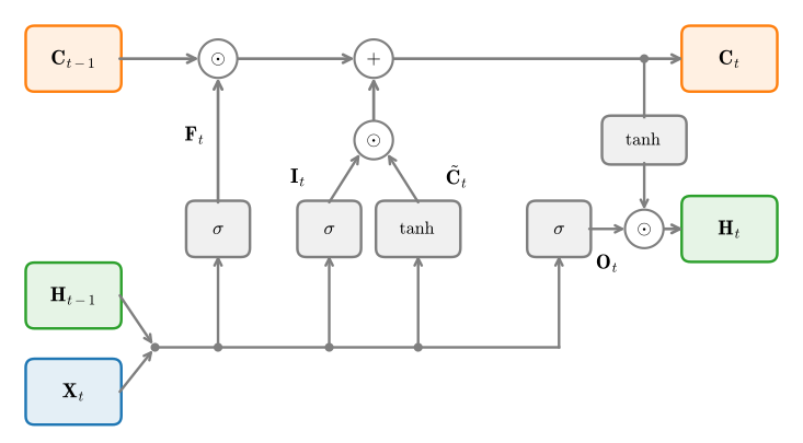
Follow the top path of Figure 12.1.1 from left to right. The cell state is touched only by an elementwise product and an elementwise sum; no matrix multiplication and no saturating nonlinearity stands between \(\mathbf{C}_{t-1}\) and \(\mathbf{C}_t\). Along this direct path — gates and candidate held fixed — the Jacobian is \(\partial \mathbf{C}_t / \partial \mathbf{C}_{t-1} = \textrm{diag}(\mathbf{F}_t)\), so with the forget gate near \(1\) and the input gate near \(0\) the cell holds its value, and the gradient holds with it, across arbitrarily many steps. To be precise about what is and is not guaranteed: \(\mathbf{F}_t\), \(\mathbf{I}_t\), and \(\tilde{\mathbf{C}}_t\) all depend on \(\mathbf{H}_{t-1}\), which depends on \(\mathbf{C}_{t-1}\), so the total derivative of \(\mathbf{C}_t\) with respect to \(\mathbf{C}_{t-1}\) carries additional terms that flow through the gates and reintroduce exactly the matrix products the direct path avoids (Section 24.2.2 analyzes such Jacobian products). The architecture supplies a well-conditioned additive route and lets learning control it; it does not guarantee that every gradient is preserved. This protected additive path is the constant error carousel that gives the LSTM its resistance to vanishing gradients: it is precisely the controlled accumulator we asked for. The output gate adds a subtler ability: a cell can accumulate evidence silently for many steps (\(\mathbf{O}_t \approx 0\)), invisible to the layers above, and release it at the moment it becomes relevant. Only \(\mathbf{H}_t\) is passed to output layers and to the next stacked layer; the cell state stays internal to the cell.
12.1.2.2 Implementation from Scratch
We implement the cell using the template of Section 8.5: the cell class holds parameters and steps the recurrence, and d2l.RNNLMScratch wraps it with an embedding and an output head to form a language model. As there, num_inputs is the width of the vectors the cell consumes at each step, which will be the embedding dimension. Each of the four heads needs the same triple of parameters, so we build them with a small factory.
class LSTMScratch(d2l.Module):
    """The long short-term memory (LSTM) cell implemented from scratch."""
    def __init__(self, num_inputs, num_hiddens, sigma=0.01):
        super().__init__()
        self.save_hyperparameters()

        init_weight = lambda *shape: nn.Parameter(d2l.randn(*shape) * sigma)
        triple = lambda: (init_weight(num_inputs, num_hiddens),
                          init_weight(num_hiddens, num_hiddens),
                          nn.Parameter(d2l.zeros(num_hiddens)))
        self.W_xi, self.W_hi, self.b_i = triple()  # Input gate
        self.W_xf, self.W_hf, self.b_f = triple()  # Forget gate
        self.W_xo, self.W_ho, self.b_o = triple()  # Output gate
        self.W_xc, self.W_hc, self.b_c = triple()  # Input node
class LSTMScratch(nnx.Module):
"""The long short-term memory (LSTM) cell implemented from scratch."""
def __init__(self, num_inputs, num_hiddens, sigma=0.01, rngs=None):
rngs = nnx.Rngs(0) if rngs is None else rngs
self.num_inputs, self.num_hiddens = num_inputs, num_hiddens
self.sigma = sigma
init_weight = lambda shape: nnx.Param(
rngs.params.normal(shape) * sigma)
triple = lambda: (
init_weight((num_inputs, num_hiddens)),
init_weight((num_hiddens, num_hiddens)),
nnx.Param(jnp.zeros(num_hiddens)))
self.W_xi, self.W_hi, self.b_i = triple() # Input gate
self.W_xf, self.W_hf, self.b_f = triple() # Forget gate
self.W_xo, self.W_ho, self.b_o = triple() # Output gate
self.W_xc, self.W_hc, self.b_c = triple() # Input nodeThe forward computation walks the time axis just as the vanilla cell did, except that each step evaluates Equation 12.1.3, Equation 12.1.4, and Equation 12.1.5, and the carried state is now the pair \((\mathbf{H}, \mathbf{C})\).
The explicit Python loop of the other tab is the readable teaching form, but under JIT compilation it is unrolled into a graph that grows with the sequence length, which for the LSTM’s eight matrix products per step makes compilation painfully slow. As promised in Section 8.5, we switch to jax.lax.scan: it takes a step function, an initial carry, and an array whose leading axis is scanned, and returns the final carry with the stacked per-step outputs.
@d2l.add_to_class(LSTMScratch)
def forward(self, inputs, H_C=None):
    if H_C is None:
        # Initial state with shape: (batch_size, num_hiddens)
        H = d2l.zeros((inputs.shape[1], self.num_hiddens),
                      device=inputs.device)
        C = d2l.zeros((inputs.shape[1], self.num_hiddens),
                      device=inputs.device)
    else:
        H, C = H_C
    outputs = []
    for X in inputs:
        I = d2l.sigmoid(d2l.matmul(X, self.W_xi) +
                        d2l.matmul(H, self.W_hi) + self.b_i)
        F = d2l.sigmoid(d2l.matmul(X, self.W_xf) +
                        d2l.matmul(H, self.W_hf) + self.b_f)
        O = d2l.sigmoid(d2l.matmul(X, self.W_xo) +
                        d2l.matmul(H, self.W_ho) + self.b_o)
        C_tilde = d2l.tanh(d2l.matmul(X, self.W_xc) +
                           d2l.matmul(H, self.W_hc) + self.b_c)
        C = F * C + I * C_tilde
        H = O * d2l.tanh(C)
        outputs.append(H)
return outputs, (H, C)@d2l.add_to_class(LSTMScratch)
def __call__(self, inputs, H_C=None):
def scan_fn(H_C, X):
H, C = H_C
I = d2l.sigmoid(d2l.matmul(X, self.W_xi) +
d2l.matmul(H, self.W_hi) + self.b_i)
F = d2l.sigmoid(d2l.matmul(X, self.W_xf) +
d2l.matmul(H, self.W_hf) + self.b_f)
O = d2l.sigmoid(d2l.matmul(X, self.W_xo) +
d2l.matmul(H, self.W_ho) + self.b_o)
C_tilde = d2l.tanh(d2l.matmul(X, self.W_xc) +
d2l.matmul(H, self.W_hc) + self.b_c)
C = F * C + I * C_tilde
H = O * d2l.tanh(C)
return (H, C), H # Return (carry, per-step output)
if H_C is None:
batch_size = inputs.shape[1]
H_C = (jnp.zeros((batch_size, self.num_hiddens)),
jnp.zeros((batch_size, self.num_hiddens)))
H_C, outputs = jax.lax.scan(scan_fn, H_C, inputs)
return outputs, H_CA quick shape check confirms that the cell consumes a (num_steps, batch_size, num_inputs) tensor and that both pieces of state keep the (batch_size, num_hiddens) shape from step to step.
lstm = LSTMScratch(num_inputs=16, num_hiddens=32)
X = d2l.ones((9, 4, 16))  # (num_steps, batch_size, num_inputs)
outputs, (H, C) = lstm(X)
d2l.check_shape(outputs[-1], (4, 32))
d2l.check_shape(H, (4, 32))
d2l.check_shape(C, (4, 32))
lstm = LSTMScratch(num_inputs=16, num_hiddens=32)
X = d2l.ones((9, 4, 16)) # (num_steps, batch_size, num_inputs)
outputs, (H, C) = lstm(X)
d2l.check_shape(outputs[-1], (4, 32))
d2l.check_shape(H, (4, 32))
d2l.check_shape(C, (4, 32))12.1.2.3 Training
Does the gated cell actually beat the vanilla RNN? To make the comparison mean something we reuse the recipe of Section 8.5 unchanged: The Time Machine under the 1,024-token BPE tokenizer, 50,000 training windows of 32 tokens, embedding dimension 64, 128 hidden units, ten epochs with gradients clipped to norm 1.
data = d2l.TimeMachine(batch_size=1024, num_steps=32,
                       num_train=50000, num_val=5000)
data = d2l.TimeMachine(batch_size=1024, num_steps=32,
num_train=50000, num_val=5000)The language-model scaffold from Section 8.5 accepts the new cell without modification, because the cell keeps the same interface: embeddings in, per-step hidden states out. Only the recurrence changed.
lstm = LSTMScratch(num_inputs=64, num_hiddens=128)
model = d2l.RNNLMScratch(lstm, vocab_size=len(data.vocab), lr=4)
lstm = LSTMScratch(num_inputs=64, num_hiddens=128)
model = d2l.RNNLMScratch(lstm, vocab_size=len(data.vocab), lr=4)trainer = d2l.Trainer(max_epochs=10, gradient_clip_val=1, num_gpus=1)
model.board.yscale = 'log'
trainer.fit(model, data)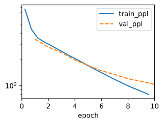
trainer = d2l.Trainer(max_epochs=10, gradient_clip_val=1, num_gpus=1)
model.board.yscale = 'log'
trainer.fit(model, data)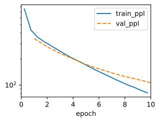
We will train several models in this section, so we wrap the perplexity readout in a helper and start a small scoreboard.
def val_ppl(model):
return float(model.board.data['val_ppl'][-1].y)
ppls = {'LSTM (scratch)': val_ppl(model)}
print(f"validation perplexity {ppls['LSTM (scratch)']:.1f}")validation perplexity 104.7def val_ppl(model):
total_loss = num_tokens = 0
for X_val, y_val in data.val_dataloader():
losses = model.loss(model(X_val), y_val, averaged=False)
total_loss += float(losses.sum())
num_tokens += losses.size
return math.exp(total_loss / num_tokens)
ppls = {'LSTM (scratch)': val_ppl(model)}
print(f"validation perplexity {ppls['LSTM (scratch)']:.1f}")validation perplexity 103.8Under the identical recipe, the vanilla RNN of Section 8.5 reached a validation perplexity in the neighborhood of 90 to 110, and our from-scratch LSTM lands in the same range. Two factors limit this run. First, ten epochs is a short budget for a cell whose recurrent core has four heads and \(4h(d + h + 1)\) weights instead of \(h(d + h + 1)\): the curves are still moving when the budget ends, so the model is undertrained rather than out of capacity. Second, our naive initialization starts every gate half-open: with weights near zero, \(\sigma(0) = 0.5\), so the untrained forget gate halves the cell state at every step, and the carousel only starts carrying once training pushes the forget-gate biases up. Practitioners initialize \(\mathbf{b}_\textrm{f}\) to 1 for exactly this reason, and an exercise asks you to try both remedies. Under this section’s fixed budget, the streamlined GRU below provides the clearest comparison with the vanilla RNN.
12.1.2.4 Concise Implementation
Every framework ships an LSTM layer that fuses the cell and the time loop into one optimized call; as Section 8.5 measured for the vanilla cell, the fused kernel is what you use for any model you train at length, and for the LSTM the gap is larger because each hand-rolled step launches eight matrix products. The LSTM class below keeps the interface of LSTMScratch and adds a num_layers argument, which stacks recurrent layers on top of one another; we use it later in this section, and the following sections of this chapter reuse it as their recurrent baseline. As before, num_inputs is the width of the per-step input vectors.
class LSTM(d2l.RNN):
"""The multilayer LSTM model implemented with high-level APIs."""
def __init__(self, num_inputs, num_hiddens, num_layers=1, dropout=0):
d2l.Module.__init__(self)
self.save_hyperparameters()
self.rnn = nn.LSTM(num_inputs, num_hiddens, num_layers,
dropout=dropout)
def forward(self, inputs, H_C=None):
return self.rnn(inputs, H_C)class LSTM(d2l.RNN):
"""The multilayer LSTM model implemented with high-level APIs."""
def __init__(self, num_inputs, num_hiddens, num_layers=1, dropout=0,
rngs=None):
rngs = nnx.Rngs(params=0, dropout=1, carry=2) if rngs is None \
else rngs
self.num_inputs, self.num_hiddens = num_inputs, num_hiddens
self.num_layers = num_layers
self.rnns = nnx.List([
nnx.RNN(nnx.LSTMCell(num_inputs if i == 0 else num_hiddens,
num_hiddens, rngs=rngs),
time_major=True, return_carry=True, rngs=rngs)
for i in range(num_layers)])
self.dropouts = nnx.List([
nnx.Dropout(dropout, rngs=rngs) for _ in range(num_layers - 1)])
def __call__(self, inputs, H_C=None):
outputs = inputs
H_C = [None] * self.num_layers if H_C is None else H_C
new_H_C = []
for i, rnn in enumerate(self.rnns):
carry, outputs = rnn(outputs, initial_carry=H_C[i])
new_H_C.append(carry)
if i < self.num_layers - 1:
outputs = self.dropouts[i](outputs)
return outputs, new_H_CThe concise language model d2l.RNNLM wraps it exactly as its scratch counterpart did, and training is the same call with the same hyperparameters.
lstm = LSTM(num_inputs=64, num_hiddens=128)
model = d2l.RNNLM(lstm, vocab_size=len(data.vocab), lr=4)lstm = LSTM(num_inputs=64, num_hiddens=128)
model = d2l.RNNLM(lstm, vocab_size=len(data.vocab), lr=4)trainer = d2l.Trainer(max_epochs=10, gradient_clip_val=1, num_gpus=1)
model.board.yscale = 'log'
trainer.fit(model, data)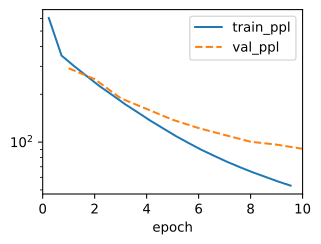
trainer = d2l.Trainer(max_epochs=10, gradient_clip_val=1, num_gpus=1)
model.board.yscale = 'log'
trainer.fit(model, data)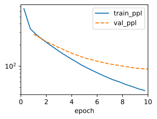
The trained model reaches a somewhat better perplexity than our from-scratch cell. The difference is not the arithmetic, which is identical, but the starting point, and it is worth being precise about what each framework actually does. PyTorch’s nn.LSTM draws every weight and bias uniformly at scale \(1/\sqrt{h}\); Flax’s LSTMCell pairs fan-in-scaled input weights with orthogonal recurrent matrices and zero biases. Both are better starting points than our teaching code’s small Gaussian, and they differ from each other — one reason the two tabs’ numbers do not match. Note what neither default includes: the forget-gate bias of 1 recommended above remains yours to set. At a fixed training budget, how you start matters.
Reading the perplexity off the scoreboard, we let the model continue the time traveller. As Section 8.5 explained, greedy (argmax) decoding of a model this lightly trained soon drifts into a repetition loop, so we sample at a low temperature: the continuation stays close to the model’s preferences yet keeps moving.
ppls['LSTM'] = val_ppl(model)
pred = model.predict('the time traveller', 30, data.tokenizer, d2l.try_gpu(),
temperature=0.5)
d2l.print_wrapped(f"perplexity {ppls['LSTM']:.1f}, {pred!r}")perplexity 96.0, 'the time travellerlour\nof the fainthy. I remember\nI had
a faintached down the\ndestion of'ppls['LSTM'] = val_ppl(model)
pred = model.predict('the time traveller', 30, data.tokenizer,
temperature=0.5)
d2l.print_wrapped(f"perplexity {ppls['LSTM']:.1f}, {pred!r}")perplexity 93.1, 'the time travellering a fair\nof trailing to the Palace of
the hall, and now, but\nI could see, I'12.1.3 Gated Recurrent Units
As LSTMs spread through the 2010s, researchers looked for cheaper cells that kept the two essential ingredients, an additive state path and multiplicative gates. The most widely used answer is the gated recurrent unit (GRU) of Cho et al. (2014): it drops the separate cell state, letting the hidden state itself be the memory, and merges four heads into three. Early comparisons found that this reduction could match LSTM quality on several tasks (Chung et al. 2014).
12.1.3.1 Reset and Update Gates
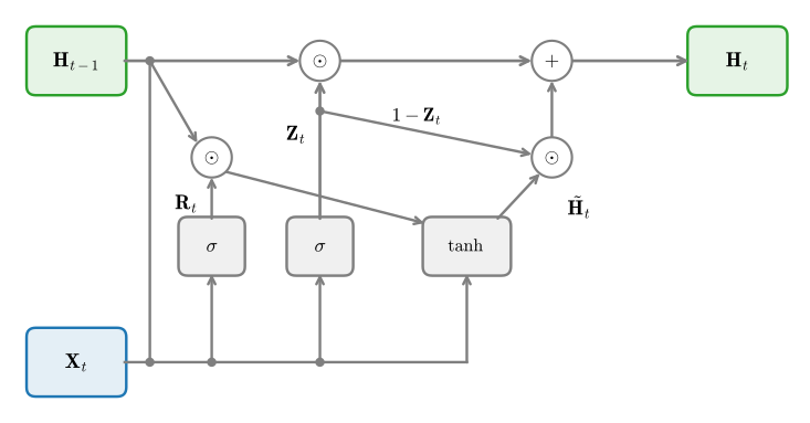
The GRU computes two gates in the form of Equation 12.1.2, a reset gate \(\mathbf{R}_t\) and an update gate \(\mathbf{Z}_t\):
\[ \mathbf{R}_t = \sigma(\mathbf{X}_t \mathbf{W}_{\textrm{xr}} + \mathbf{H}_{t-1} \mathbf{W}_{\textrm{hr}} + \mathbf{b}_\textrm{r}), \qquad \mathbf{Z}_t = \sigma(\mathbf{X}_t \mathbf{W}_{\textrm{xz}} + \mathbf{H}_{t-1} \mathbf{W}_{\textrm{hz}} + \mathbf{b}_\textrm{z}). \tag{12.1.6}\]
The reset gate acts inside the candidate state: it filters how much of the previous state may enter the vanilla-RNN-style proposal,
\[ \tilde{\mathbf{H}}_t = \tanh(\mathbf{X}_t \mathbf{W}_{\textrm{xh}} + \left(\mathbf{R}_t \odot \mathbf{H}_{t-1}\right) \mathbf{W}_{\textrm{hh}} + \mathbf{b}_\textrm{h}), \tag{12.1.7}\]
so \(\mathbf{R}_t \approx 1\) recovers the vanilla recurrence while \(\mathbf{R}_t \approx 0\) makes the proposal a function of the current input alone, as if the sequence restarted. The update gate then blends old state and proposal as a convex combination,
\[ \mathbf{H}_t = \mathbf{Z}_t \odot \mathbf{H}_{t-1} + (1 - \mathbf{Z}_t) \odot \tilde{\mathbf{H}}_t. \tag{12.1.8}\]
Here the additive memory path is plain to see: wherever \(\mathbf{Z}_t \approx 1\) the new state is a copy of the old one and the step is effectively skipped, giving the same near-identity direct-path Jacobian as the LSTM’s carousel (with the same caveat: the gates themselves depend on \(\mathbf{H}_{t-1}\), so this is the protected route, not the total derivative); wherever \(\mathbf{Z}_t \approx 0\) the state is overwritten by the proposal. Because Equation 12.1.8 is a convex combination of two bounded quantities, the state stays bounded by construction, and the GRU needs neither a separate protected accumulator nor an output squashing: one vector serves as memory and output at once. The division of labor is that reset gates capture short-range decisions (what to drop from the proposal) and update gates capture long-range ones (how long to hold state). Figure 12.1.2 shows the flow.
12.1.3.2 Implementation and Comparison
After the LSTM, a from-scratch GRU offers no new idea, only one fewer head, so we skip straight to the framework layer (an exercise asks you to write the scratch version by editing LSTMScratch). The class mirrors LSTM, including the num_layers argument; the GRU is also the cell that the next section (Section 12.2) strips down to its minimal linear core.
class GRU(d2l.RNN):
"""The multilayer GRU model implemented with high-level APIs."""
def __init__(self, num_inputs, num_hiddens, num_layers=1, dropout=0):
d2l.Module.__init__(self)
self.save_hyperparameters()
self.rnn = nn.GRU(num_inputs, num_hiddens, num_layers,
dropout=dropout)class GRU(d2l.RNN):
"""The multilayer GRU model implemented with high-level APIs."""
def __init__(self, num_inputs, num_hiddens, num_layers=1, dropout=0,
rngs=None):
rngs = nnx.Rngs(params=0, dropout=1, carry=2) if rngs is None \
else rngs
self.num_inputs, self.num_hiddens = num_inputs, num_hiddens
self.num_layers = num_layers
self.rnns = nnx.List([
nnx.RNN(nnx.GRUCell(num_inputs if i == 0 else num_hiddens,
num_hiddens, rngs=rngs),
time_major=True, return_carry=True, rngs=rngs)
for i in range(num_layers)])
self.dropouts = nnx.List([
nnx.Dropout(dropout, rngs=rngs) for _ in range(num_layers - 1)])
def __call__(self, X, state=None):
outputs = X
state = [None] * self.num_layers if state is None else state
new_state = []
for i, rnn in enumerate(self.rnns):
carry, outputs = rnn(outputs, initial_carry=state[i])
new_state.append(carry)
if i < self.num_layers - 1:
outputs = self.dropouts[i](outputs)
return outputs, new_stateOne training run under the same recipe puts the GRU on our scoreboard.
gru = GRU(num_inputs=64, num_hiddens=128)
model = d2l.RNNLM(gru, vocab_size=len(data.vocab), lr=4)gru = GRU(num_inputs=64, num_hiddens=128)
model = d2l.RNNLM(gru, vocab_size=len(data.vocab), lr=4)trainer = d2l.Trainer(max_epochs=10, gradient_clip_val=1, num_gpus=1)
model.board.yscale = 'log'
trainer.fit(model, data)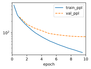
trainer = d2l.Trainer(max_epochs=10, gradient_clip_val=1, num_gpus=1)
model.board.yscale = 'log'
trainer.fit(model, data)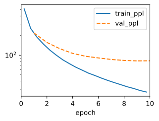
ppls['GRU'] = val_ppl(model)
print(f"validation perplexity {ppls['GRU']:.1f}")validation perplexity 79.0ppls['GRU'] = val_ppl(model)
print(f"validation perplexity {ppls['GRU']:.1f}")validation perplexity 81.8At the same width the GRU’s recurrent core has \(3h(d + h + 1)\) weights to the LSTM’s \(4h(d + h + 1)\) and computes three matmul heads per step instead of four, yet in our runs it posts the best perplexity of the section, ahead of the vanilla RNN and the LSTM at this budget. This short schedule measures convergence rather than ultimate capacity. The GRU has fewer gates to coordinate, and its convex state blend remains well scaled from the first epoch. This mirrors the early empirical comparisons (Chung et al. 2014), which found the GRU at least the LSTM’s equal on small and mid-sized tasks; with longer training and careful initialization the LSTM closes the gap (see the exercises).
Equation Equation 12.1.8 also points toward later linear recurrences. The only nonlinearity standing between \(\mathbf{H}_{t-1}\) and \(\mathbf{H}_t\) enters through \(\tilde{\mathbf{H}}_t\) and the gates. If one makes the gates functions of the input alone and lets the candidate ignore the previous state, the update becomes linear in \(\mathbf{H}_{t-1}\), and a linear recurrence can be trained in parallel across the whole sequence rather than step by step. That observation is the seed of minimal gated cells such as minGRU (Feng et al. 2024), of linear recurrent units (Orvieto et al. 2023), and of the state space models that now appear inside production language models, and Section 12.2 works it out in full. The GRU therefore connects the gated LSTM to the linear recurrences that follow.
12.1.4 Depth and Direction
Gating changes what happens inside a cell; two further RNN-era design axes change how cells are wired together. We compress both to the lessons that outlived them.
12.1.4.1 Deep Recurrent Networks
A deep RNN stacks recurrent layers, each reading the hidden-state sequence of the layer below as its input sequence: function composition within a time step, on top of recurrence across steps. Gated cells handle the time direction; the layer direction borrows the feedforward remedies of residual connections (Section 7.4) and between-layer dropout. For recurrent models, stacks beyond four to eight layers rarely paid off. Since our LSTM class already accepts num_layers, a two-layer model is a one-argument change, and it completes our scoreboard.
lstm2 = LSTM(num_inputs=64, num_hiddens=128, num_layers=2)
model = d2l.RNNLM(lstm2, vocab_size=len(data.vocab), lr=4)
trainer = d2l.Trainer(max_epochs=10, gradient_clip_val=1, num_gpus=1)
model.board.yscale = 'log'
trainer.fit(model, data)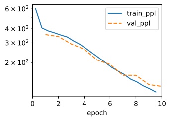
lstm2 = LSTM(num_inputs=64, num_hiddens=128, num_layers=2)
model = d2l.RNNLM(lstm2, vocab_size=len(data.vocab), lr=4)
trainer = d2l.Trainer(max_epochs=10, gradient_clip_val=1, num_gpus=1)
model.board.yscale = 'log'
trainer.fit(model, data)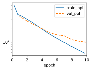
ppls['LSTM (2 layers)'] = val_ppl(model)
print(f'{"model":>16} {"val ppl":>8}')
for name, p in ppls.items():
    print(f'{name:>16} {p:>8.1f}')
model val ppl
LSTM (scratch) 104.7
LSTM 96.0
GRU 79.0
LSTM (2 layers) 123.6ppls['LSTM (2 layers)'] = val_ppl(model)
print(f'{"model":>16} {"val ppl":>8}')
for name, p in ppls.items():
print(f'{name:>16} {p:>8.1f}') model val ppl
LSTM (scratch) 103.8
LSTM 93.1
GRU 81.8
LSTM (2 layers) 98.2The results require a narrow interpretation. The GRU beats the vanilla RNN of Section 8.5 clearly at the same recipe; the single-layer LSTM roughly matches the vanilla model within this short budget, for the initialization and budget reasons discussed above; and the second layer does not improve validation perplexity under this recipe. It adds parameters and optimization work that this small corpus and short training budget do not use effectively. This result does not imply that depth is unhelpful on larger corpora or with longer training.
12.1.4.2 Bidirectional Recurrent Networks
Language modeling forces left-to-right reading, but a model that analyzes a complete, given sequence has the future context in hand, and that context is informative. Part-of-speech tagging is one such task. A bidirectional RNN (Schuster and Paliwal 1997) runs a second, independent recurrent layer backward over the same input and concatenates the two states at each step into \(\mathbf{H}_t = [\overrightarrow{\mathbf{H}}_t, \overleftarrow{\mathbf{H}}_t] \in \mathbb{R}^{n \times 2h}\): every output conditions on the entire sequence, at twice the compute. In frameworks this is a flag or a wrapper, and the shape check shows exactly what changed, the per-step output width doubling to \(2h\).
birnn = nn.LSTM(64, 128, bidirectional=True)
X = d2l.randn(32, 8, 64)  # (num_steps, batch_size, num_inputs)
outputs, (H, C) = birnn(X)
outputs.shape, H.shape
(torch.Size([32, 8, 256]), torch.Size([2, 8, 128]))birnn = nnx.Bidirectional(
nnx.RNN(nnx.LSTMCell(64, 128, rngs=nnx.Rngs(0)),
time_major=True, rngs=nnx.Rngs(0)),
nnx.RNN(nnx.LSTMCell(64, 128, rngs=nnx.Rngs(1)), time_major=True,
reverse=True, keep_order=True, rngs=nnx.Rngs(1)),
time_major=True)
X = jax.random.normal(d2l.get_key(), (32, 8, 64))
outputs = birnn(X)
outputs.shape(32, 8, 256)One warning matters more than the mechanics: a bidirectional network cannot serve unchanged as a causal decoder. Every \(\mathbf{H}_t\) conditions on tokens after \(t\), so the model cannot emit tokens left-to-right autoregressively because future tokens are unavailable. Training such a model to predict the next token also leaks the target: the backward recurrence receives that token as part of its input. The resulting low training loss therefore does not measure causal prediction, and the model cannot be used unchanged for left-to-right generation. The scope of the warning is the causal role, not generation wholesale: bidirectional encoders live inside generative systems (the encoder half of a translation model conditions a causal decoder), and non-autoregressive decoders generate whole sequences by iterative refinement rather than left to right. Use bidirectional layers where the full input is given up front and per-position representations are wanted: tagging, span labeling, and encoding. Their most consequential success was ELMo (Peters et al. 2018), deep bidirectional LSTMs trained to produce contextual word embeddings (see also (Graves and Schmidhuber 2005)); the bidirectional attention of BERT (Devlin et al. 2018) then inherited that role and the entire encode-both-directions idea, and we study BERT in the pretraining chapters.
12.1.5 Gates in Other Architectures
The cells above are, by the standards of this book’s earlier chapters, old technology. The gate is not. Its shape is a sigmoid (or other bounded) branch elementwise-multiplying a signal branch, and once you know that shape you will find it across modern deep learning, doing the same job of content-dependent routing that it does inside the LSTM.
Highway networks (Srivastava et al. 2015) applied the LSTM’s gating to depth: a transform gate blends each layer’s output with its unmodified input, letting very deep feedforward networks train years before normalization made it routine, and prefiguring the residual connections of Section 7.4. Transformer blocks carry gates in their MLPs: the gated linear unit family is the standard MLP in most contemporary open language models, its SwiGLU variant (Shazeer 2020) computing \(\textrm{Swish}(\mathbf{x}\mathbf{W}_1) \odot \mathbf{x}\mathbf{W}_2\); Section 11.1 measured the effect of that gate in a matched-parameter sweep. And the recurrence story of this chapter continues the pattern most directly: the selective state space model Mamba (Gu and Dao 2023) modulates a linear state with an input-dependent step size \(\Delta_t\) that plays precisely the role of a forget gate, and Griffin (De et al. 2024) builds production-scale hybrids from gated linear recurrences.
The gate even circled back to the cell it came from. xLSTM (Beck et al. 2024) revisits the LSTM with exponential gating: its sLSTM cell replaces the sigmoid’s \((0,1)\) range with \(\exp\), so a confident new write can overwhelm the accumulated state rather than merely dilute it, and a running maximum carried in log space keeps the unbounded gates numerically stable. The result revives the classic recurrent, state-dependent cell at modern scale. Its sibling, the matrix-memory mLSTM, gives up state-dependent gating to regain parallel training, and appears where it belongs, in the family table of Section 12.4. One idea, many guises:
| Where | The gate | What it controls |
|---|---|---|
| LSTM (1997) | forget gate \(\mathbf{F}_t\) | decay of the cell state \(\mathbf{C}_t\) |
| GRU (2014) | update gate \(\mathbf{Z}_t\) | copy-vs-overwrite blend of \(\mathbf{H}_t\) |
| Highway nets (2015) | transform gate | skip-vs-transform blend across depth |
| GLU, SwiGLU MLPs (Section 11.1) | activation branch | which channels pass through the MLP |
| Mamba (2023) | step size \(\Delta_t\) | decay of a linear state, from input only |
| Griffin, mLSTM (2024) | recurrence gates | decay and write strength of linear cells |
The gates in the last three rows depend on the input only, not on the state. Removing state-dependent gating makes the recurrence linear. The result permits parallel training across the sequence while retaining learned forgetting. Section 12.2 takes exactly that step, and the rest of the chapter rides it: linear state space models, made selective in Section 12.3, reconciled with attention in Section 12.4, taught to edit their memory in Section 12.5, reread as learning at test time in Section 12.6, and finally hybridized with the transformer in Section 12.7. Input-dependent gating provides the starting point for that comparison.
12.1.6 Summary
Gating addresses vanishing gradients by maintaining an additive state path whose direct-path Jacobian stays near the identity and controlling reads, writes, and erasures with learned sigmoid gates that multiply elementwise. The LSTM realizes this with a protected cell state and three gates; its cell update \(\mathbf{C}_t = \mathbf{F}_t \odot \mathbf{C}_{t-1} + \mathbf{I}_t \odot \tilde{\mathbf{C}}_t\) is the constant error carousel that lets both information and gradients cross long horizons. The GRU reaches nearly the same behavior with two gates and no separate cell, at three quarters of the recurrent parameters. On an identical short training recipe the GRU clearly outperforms the vanilla RNN from Section 8.5, while the LSTM needs a longer budget or a friendlier initialization before its extra machinery pays: architecture and optimization cannot be judged separately. Depth and bidirectionality are orthogonal wiring choices: stacked layers in the first case, a backward pass concatenated to the forward one in the second. Bidirectionality yields encoders, which cannot double unchanged as causal decoders. The gate itself outlived these architectures: it routes channels in transformer MLPs (Section 11.1), revives the LSTM in exponential form (xLSTM), and, made input-dependent only, powers the linear recurrences and state space models that the rest of this chapter builds.
Experimental scope. Under one fixed small-corpus recipe, gate-equipped cells train reliably where the vanilla RNN plateaus, and initialization can matter as much as architecture at a ten-epoch budget. These are single seeded runs on one small corpus: they do not rank LSTM against GRU in general, and they say nothing about behavior at scale, where budgets, tuning, and data change the ordering.
12.1.7 Exercises
- Holding a value. Suppose that the token at step \(t'\) determines the prediction at a much later step \(t\), and that one memory cell is to carry it from \(t'\) to \(t\).
- State the value that each gate of that cell in Equation 12.1.3 should take at step \(t'\), at the steps strictly between \(t'\) and \(t\), and at step \(t\). Then do the same for the update gate of a GRU unit in Equation 12.1.8.
- A sigmoid gate never reaches 1. Suppose that the forget gate’s pre-activation stays at a constant \(b\), so that its value is \(\sigma(b)\) at every step. What fraction of the stored value survives \(k\) steps along the direct path? How large must \(b\) be for 90% of the value to survive 1,000 steps?
- Show that a forget-gate bias of \(\log(T - 1)\) gives an initial forget gate of \(1 - 1/T\) when the weights are zero, so that for large \(T\) a stored value decays by a factor of about \(e\) over \(T\) steps. The chrono initialization of Tallec and Ollivier (2018) draws the forget-gate bias of each unit as \(\log u\), with \(u\) uniform on \([1, T_\textrm{max} - 1]\), and sets \(\mathbf{b}_\textrm{i} = -\mathbf{b}_\textrm{f}\). Show that with zero weights this makes \(\mathbf{F}_t + \mathbf{I}_t = 1\), and compare the resulting cell update with Equation 12.1.8.
- [code] The carousel’s other paths. ● Consider an LSTM with one input and one hidden unit, so that every quantity in Equation 12.1.3, Equation 12.1.4, and Equation 12.1.5 is a scalar. Write \(C_t\), \(H_t\), \(F_t\), \(I_t\), \(O_t\), and \(\tilde{C}_t\) for these scalars, and \(w_\textrm{hf}\), \(w_\textrm{hi}\), and \(w_\textrm{hc}\) for the recurrent weights of the forget gate, the input gate, and the input node.
- The output gate \(O_{t-1}\) depends on \(H_{t-2}\) but not on \(C_{t-1}\). Using \(H_{t-1} = O_{t-1} \tanh(C_{t-1})\), derive the total derivative \(\textrm{d}C_t / \textrm{d}C_{t-1}\). Write it as the direct-path value \(F_t\) plus a correction, and factor the correction into a term from step \(t\) and the derivative \(\textrm{d}H_{t-1} / \textrm{d}C_{t-1}\).
- For which values of the gates, of \(\tilde{C}_t\), and of \(C_{t-1}\) does the correction vanish? Which of these conditions can the network set through its gates while the cell is storing a value?
- Now compare the two paths in a trained model. Train
LSTMScratchwith the recipe of Section 12.1.2.3, and let it read 1,024 consecutive validation tokens with the state carried across them. Compute the norm of the gradient of the loss at the last token with respect to \(\mathbf{C}_{1024-k}\) for \(k\) up to 256, and plot it against \(k\) on a logarithmic scale. Compare it with the gradient carried by the direct path alone, which multiplies the gradient at \(\mathbf{C}_{1024}\) elementwise by the product of the forget-gate values over the last \(k\) steps. Where do the two curves part, and which is larger?
- Output squashing. The input node \(\tilde{\mathbf{C}}_t\) is already squashed by the \(\tanh\) in Equation 12.1.4, yet Equation 12.1.5 applies \(\tanh\) to \(\mathbf{C}_t\) again before the output gate.
- Starting from \(\mathbf{C}_0 = \mathbf{0}\), show that every entry of \(\mathbf{C}_t\) is smaller than \(t\) in magnitude. Show further that if every forget-gate value is at most \(f_\textrm{max} < 1\), every entry stays below \(1 / (1 - f_\textrm{max})\) in magnitude, whatever \(t\) is.
- Suppose that the hidden state were \(\mathbf{H}_t = \mathbf{O}_t \odot \mathbf{C}_t\) instead. After many steps of accumulation, what happens to the gate pre-activations at the next step, and what does that do to the gradients that flow through the gates?
- [code] Forget-gate bias. With weights near zero, the forget gate is close to \(\sigma(\mathbf{b}_\textrm{f})\), so
LSTMScratchstarts with every forget gate near \(0.5\). Jozefowicz et al. (2015) found that a forget-gate bias of 1 let the LSTM nearly match the GRU on their benchmarks.- Initialize \(\mathbf{b}_\textrm{f}\) to 1 in
LSTMScratch, keep the other biases at zero, and train with the recipe of Section 12.1.2.3. Compare the validation perplexity with that of the run with \(\mathbf{b}_\textrm{f} = \mathbf{0}\), and repeat both runs with a second random seed. Does the difference exceed the spread between seeds? - Train both initializations and
GRUfor 20 epochs instead of 10, and plot the validation perplexity of all three after every epoch. Which of the two remedies, the bias or the longer budget, closes more of the gap between the LSTM and the lowest validation perplexity that the GRU reaches at any epoch? - Set the total forget-gate bias of the concise
LSTMto 1 at initialization and retrain it. The fused layer keeps its gate parameters in its own layout and initializes them differently fromLSTMScratch(Section 12.1.2.4), so locate the forget-gate bias first. Does the change help the concise model?
- Initialize \(\mathbf{b}_\textrm{f}\) to 1 in
- [code] No forget gate. ● The original LSTM of Hochreiter and Schmidhuber (1997) had no forget gate; Gers et al. (2000) added it.
- Remove the forget gate’s parameters from
LSTMScratchand use \(\mathbf{F}_t = 1\) in Equation 12.1.5. Train with the recipe of Section 12.1.2.3 and compare the validation perplexity with that of the gated cell. - For both models, record the fraction of entries \(c_{t,i}\) of \(\mathbf{C}_t\) with \(|\tanh(c_{t,i})| > 0.99\) after the last token of the validation windows. Use the result to explain the perplexity gap.
- Each training window starts from a zero state, so neither model runs more than 32 steps without a reset during training. Take 1,024 consecutive tokens from the validation part of the corpus and evaluate each model on them twice: once with the state carried across all 1,024 tokens, and once with the state reset every 32 tokens. Report the largest \(|c_{t,i}|\) at the end of the carried run and the average loss under both schemes. Does the carried state hurt the model without a forget gate, and why or why not?
- Remove the forget gate’s parameters from
- [code] Memory timescales. In a gated cell each unit has its own learned rate of decay. Train
LSTMScratchwith the recipe of Section 12.1.2.3, let it read 1,024 consecutive validation tokens with the state carried across them, and record \(\mathbf{F}_t\) along the way.- Average the forget-gate values of each unit \(i\) to \(\bar{f}_i\), and convert each average into a time constant \(\tau_i = 1 / (1 - \bar{f}_i)\). Plot a histogram of the \(\tau_i\). How many units have a time constant longer than the 32-token training window?
- Repeat the measurement for a model trained with \(\mathbf{b}_\textrm{f}\) initialized to 1. Which parts of the timescale distribution move?
- Reset before or after. The fused layers that
GRUwraps apply the reset gate after the recurrent matrix product. Apart from the placement of the bias terms, they compute the candidate \[\tilde{\mathbf{H}}_t = \tanh(\mathbf{X}_t \mathbf{W}_{\textrm{xh}} + \mathbf{R}_t \odot (\mathbf{H}_{t-1} \mathbf{W}_{\textrm{hh}}) + \mathbf{b}_\textrm{h})\] in place of Equation 12.1.7.- Show that the two candidates agree for every \(\mathbf{R}_t\) and \(\mathbf{H}_{t-1}\) if and only if \(\mathbf{W}_{\textrm{hh}}\) is diagonal. For a general \(\mathbf{W}_{\textrm{hh}}\), which reset-gate values still make them agree?
- The input products \(\mathbf{X}_t \mathbf{W}_{\textrm{x}\cdot}\) of all steps can be computed as one large product before the recurrence starts. Under each form of the candidate, how many matrix products involving the previous state must each step perform one after the other? Why do fused GRU kernels use the form above?
- [code] GRU from scratch. Write a class
GRUScratchby editingLSTMScratch: three heads following Equation 12.1.6 and Equation 12.1.7, the update Equation 12.1.8, and a carried state that consists of \(\mathbf{H}\) alone. Keep the attributesnum_inputs,num_hiddens, andsigma, whichd2l.RNNLMScratchreads.- Check the output and state shapes as for
LSTMScratch, train the model with the recipe of Section 12.1.2.3, and compare its validation perplexity with those ofLSTMScratchand of the conciseGRU. Which of the two comparisons isolates the effect of the architecture? - Remove the reset gate by fixing \(\mathbf{R}_t = 1\), and in a second model remove the update gate by fixing \(\mathbf{Z}_t = 0\); in each case delete the parameters of the removed gate. Before training, predict from Equation 12.1.8 which removal hurts more. Then train both models, check your prediction, and explain the outcome.
- Check the output and state shapes as for
- [code] Matched parameters. Section 12.1.3 counts \(3h(d + h + 1)\) weights in the recurrent core of the GRU and \(4h(d + h + 1)\) in that of the LSTM, where \(d = 64\) is the embedding dimension.
- At \(h = 128\), find the GRU width \(h'\) whose recurrent core has about as many weights as that of the LSTM. Then count the parameters of the whole language model, including the embedding table and the output layer for the
len(data.vocab)tokens, and find the GRU width that matches whole models instead. What fraction of the parameters of the LSTM language model sits in its recurrent core? - Train the GRU at both widths with the recipe of Section 12.1.2.3 and compare with the LSTM. Does the GRU’s advantage survive either matching?
- At \(h = 128\), find the GRU width \(h'\) whose recurrent core has about as many weights as that of the LSTM. Then count the parameters of the whole language model, including the embedding table and the output layer for the
- [code] Depth sweep. ● Under the recipe of Section 12.1.2.3, the two-layer
LSTMof Section 12.1.4.1 does not improve on one layer.- Train
LSTMwithnum_layersfrom 1 to 4, and record the final training perplexity, the validation perplexity, and the time per epoch of each model. - From the gap between training and validation perplexity, decide whether the deeper models fall behind because they overfit or because they are harder to optimize within ten epochs. Test the remedy that your diagnosis suggests, either the
dropoutargument ofLSTMor a longer schedule. Do two layers then beat one?
- Train
- [code] Bidirectional leak. ● Training a bidirectional network to predict the next token leaks the target into the input, as Section 12.1.4.2 explains.
- Build a language model on a bidirectional LSTM: wrap the bidirectional layer of Section 12.1.4.2 in a class with the interface of
LSTMso thatd2l.RNNLMaccepts it, and make sure that its output layer reads \(2h\) features. Train it with the recipe of Section 12.1.2.3 and compare its training and validation perplexity with those ofLSTM. - Compute the validation loss separately for each of the 32 positions of a window. At which positions is the loss far below that of
LSTM, and at which is it not? Explain the pattern from the tokens that the backward recurrence has read at each position. - A leak-free bidirectional predictor of the token \(x_t\) combines the forward state after step \(t-1\) with the backward state after step \(t+1\), so it models the probability of \(x_t\) given all other tokens of the window. Show with a sequence of two binary tokens that the product of these conditionals over \(t\) need not sum to one over all sequences. What does this imply for using the product to score whole sequences, for instance to compare two candidate sentences or to report a perplexity?
- Build a language model on a bidirectional LSTM: wrap the bidirectional layer of Section 12.1.4.2 in a class with the interface of
- Highway gates. A highway layer (Srivastava et al. 2015) maps an input \(\mathbf{x}\) to \[\mathbf{y} = \mathbf{g} \odot \phi(\mathbf{x} \mathbf{W} + \mathbf{b}) + (1 - \mathbf{g}) \odot \mathbf{x}, \qquad \mathbf{g} = \sigma(\mathbf{x} \mathbf{W}_\textrm{g} + \mathbf{b}_\textrm{g}), \tag{12.1.9}\] where \(\phi\) is a nonlinearity and \(\mathbf{g}\) is the transform gate.
- Stack such layers and read the layer index as time. Match the stack term by term with the GRU of Equation 12.1.7 and Equation 12.1.8. Which ingredients of the GRU does the highway stack lack?
- Holding \(\mathbf{g}\) fixed, compute the Jacobian \(\partial \mathbf{y} / \partial \mathbf{x}\) and compare it with that of a residual block \(\mathbf{y} = \mathbf{x} + f(\mathbf{x})\) (Section 7.4). Which of the two layers is an accumulator in the sense of Equation 12.1.1, and which weakness of the accumulator does it inherit as the depth grows?
- Srivastava et al. (2015) initialize \(\mathbf{b}_\textrm{g}\) to a negative value. Which initialization of an LSTM gate does this correspond to, and why does it help a deep stack to train?
- [extended] Adding problem. ● Hochreiter and Schmidhuber (1997) tested long-range memory with the adding problem. A simplified version common in later work feeds two inputs per step: a value \(u_t\) drawn uniformly from \([0, 1]\) and a marker \(m_t \in \{0, 1\}\). Exactly two steps of a length-\(T\) sequence are marked, one in each half, and the target at the end of the sequence is the sum of the two marked values. A model that always predicts 1 has a mean squared error of \(1/6\).
- Write a
d2l.DataModulethat generates such sequences and a regression model that runs a recurrent layer over a sequence and applies a linear layer to its final hidden state. Train the concised2l.RNN,LSTM, andGRU, and the scratchLSTMScratch, with Adam for \(T \in \{50, 100, 200, 400\}\) under one fixed budget of epochs, and plot the validation mean squared error divided by \(1/6\) against the epoch. Up to which \(T\) does each model beat the constant prediction within the budget? - Repeat the runs of
LSTMScratchwith the forget-gate bias initialized to 1 and with the chrono initialization of Tallec and Ollivier (2018) at \(T_\textrm{max} = T\), once with the defaultsigma=0.01and once withsigma=0.1. How does each initialization change the number of epochs that the LSTM spends near the constant prediction before its error drops? How does the weight scale change the effect of the chrono initialization, and why? What do these runs say about comparing the LSTM with the GRU at a fixed budget?
- Write a