from d2l import torch as d2l
import numpy as np
import torch25.3 Matrix Calculus and Automatic Differentiation
The previous sections extended derivatives from one variable to the gradient of a scalar function of many variables. Neural network layers map vectors to vectors and often have matrix-valued parameters, so their derivatives are represented by Jacobians. This section develops matrix calculus and explains the computational cost of automatic differentiation. Backpropagation is reverse-mode automatic differentiation implemented through vector–Jacobian products, while forward mode computes Jacobian–vector products. The dimensions of a dense full Jacobian give the first cost comparison. Graph structure, repeated products, sparsity, batching, and memory can alter that choice. We also derive common matrix identities and implement both modes in compact Python examples.
We use the following imports throughout this section.
from d2l import tensorflow as d2l
import numpy as np
import tensorflow as tf
from d2l import jax as d2l
import numpy as np
import jax
from jax import numpy as jnpfrom d2l import mxnet as d2l
from mxnet import autograd, npx
from mxnet import np as mnp
import numpy as np
npx.set_np()25.3.1 Derivatives of Vector- and Matrix-Valued Maps
A layer \(\mathbf f:\mathbb R^n\to\mathbb R^m\) has one partial derivative for each input–output pair. The Jacobian organizes these derivatives and generalizes both the slope of Section 25.1 and the gradient of Section 25.2.
We use numerator layout for a vector-valued Jacobian, so \(\mathbf J_{\mathbf f}\in\mathbb R^{m\times n}\), and write the gradient of a scalar field as a column. A later reference box compares this convention with the transposed alternative.
25.3.1.1 The Jacobian as the Best Linear Approximation
In one variable, the derivative is the slope of the best straight-line fit: \(f(x+\delta)\approx f(x)+f'(x)\,\delta\). The vector-valued generalization uses the same local approximation. We say \(\mathbf f\) is differentiable at \(\mathbf x\) if there is a matrix \(\mathbf J\in\mathbb R^{m\times n}\) such that
\[ \mathbf f(\mathbf x+\boldsymbol\delta) = \mathbf f(\mathbf x) + \mathbf J\,\boldsymbol\delta + o(\|\boldsymbol\delta\|), \tag{25.3.1}\]
i.e. the error of the linear model \(\mathbf f(\mathbf x)+\mathbf J\boldsymbol\delta\) shrinks faster than \(\boldsymbol\delta\) itself as \(\boldsymbol\delta\to\mathbf 0\). That matrix, if it exists, is unique, is called the Jacobian \(\mathbf J_{\mathbf f}(\mathbf x)\), and its entries are exactly the partial derivatives:
\[ [\mathbf J_{\mathbf f}]_{ij} = \frac{\partial f_i}{\partial x_j}. \tag{25.3.2}\]
To see why, feed Equation 25.3.1 the perturbation \(\boldsymbol\delta=t\,\mathbf e_j\) (a small step along axis \(j\)) and read off component \(i\): dividing by \(t\) and letting \(t\to0\) leaves precisely \(\partial f_i/\partial x_j\) in the \((i,j)\) slot. So row \(i\) of \(\mathbf J\) collects the partials of the \(i\)-th output, and column \(j\) records how all outputs respond to nudging input \(j\). The Jacobian is the best local linear approximation; the partial-derivative formula is a consequence, not the definition.
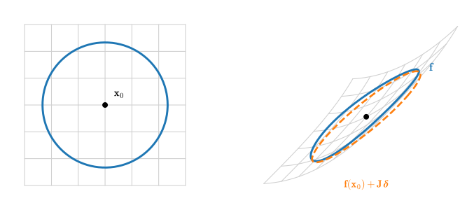
Figure 25.3.1 makes the definition visible. Up close, a differentiable map is approximated by a linear map: a small circle of inputs around \(\mathbf x_0\) maps nearly to the ellipse obtained from that circle under \(\mathbf J(\mathbf x_0)\), exactly the picture from Section 24.1 of what a matrix does to the plane. The leftover bend is the \(o(\|\boldsymbol\delta\|)\) remainder, which vanishes faster than the circle shrinks.
Two special cases recover everything we have already met. When \(m=1\) (a scalar field \(f:\mathbb R^n\to\mathbb R\)) the Jacobian is a single row, the row gradient \(\partial f/\partial\mathbf x = [\partial f/\partial x_1,\ldots,\partial f/\partial x_n]\), and Equation 25.3.1 is the first-order expansion \(f(\mathbf x+\boldsymbol\delta)\approx f(\mathbf x)+\mathbf J\boldsymbol\delta\) of Section 25.2. And the Jacobian of the gradient field \(\nabla f:\mathbb R^n\to\mathbb R^n\) is the Hessian \(\mathbf H=\mathbf J_{\nabla f}\) of Equation 25.2.7: differentiating once more turns the row gradient into the matrix of second partials, where the entry \([\mathbf J_{\nabla f}]_{ij}=\partial^2 f/\partial x_j\partial x_i\) matches the \((i,j)\) Hessian entry because mixed partials commute (Clairaut’s theorem, proved in Section 25.2). One construction, three familiar objects.
Let us pin this down on a concrete \(\mathbb R^2\to\mathbb R^2\) map and check the linear approximation against a finite difference, the numerical signature of a correct derivative.
def f(v):                                 # f: R^2 -> R^2
    x, y = v
    return np.array([x**2 * y, np.sin(x + y)])

def J(v):                                 # the exact Jacobian, entry by entry
    x, y = v
    return np.array([[2 * x * y, x**2],
                     [np.cos(x + y), np.cos(x + y)]])

x0 = np.array([1.0, 0.5])
delta = np.array([1e-3, -2e-3])
linear = f(x0) + J(x0) @ delta            # first-order prediction
exact = f(x0 + delta)                     # true value
print('linear approx:', linear.round(6))
print('exact        :', exact.round(6))
print('error / |delta|:', np.linalg.norm(exact - linear) / np.linalg.norm(delta))
linear approx: [0.499 0.997424]
exact : [0.498996 0.997424]
error / |delta|: 0.0015819444529976167The error is tiny relative to \(\|\boldsymbol\delta\|\), and shrinking it by a further factor of ten in \(\boldsymbol\delta\) shrinks the error by a factor of a hundred, the \(o(\|\boldsymbol\delta\|)\) signature of Equation 25.3.1.
25.3.1.2 The Chain Rule Is Jacobian Composition
The multivariate chain rule of Section 25.2 was a sum over paths; in matrix form it is the multiplication of Jacobians.
Proposition (chain rule). If \(\mathbf f:\mathbb R^n\to\mathbb R^p\) is differentiable at \(\mathbf x\) and \(\mathbf g:\mathbb R^p\to\mathbb R^m\) is differentiable at \(\mathbf f(\mathbf x)\), then \(\mathbf g\circ\mathbf f\) is differentiable at \(\mathbf x\) and
\[ \mathbf J_{\mathbf g\circ\mathbf f}(\mathbf x) = \mathbf J_{\mathbf g}\!\bigl(\mathbf f(\mathbf x)\bigr)\,\mathbf J_{\mathbf f}(\mathbf x). \tag{25.3.3}\]
Proof. Write \(\mathbf y=\mathbf f(\mathbf x)\) and let \(\mathbf A=\mathbf J_{\mathbf f}(\mathbf x)\), \(\mathbf B=\mathbf J_{\mathbf g}(\mathbf y)\). Linearity is the entire argument: substitute the linear model for \(\mathbf f\) into the linear model for \(\mathbf g\). By Equation 25.3.1, \(\mathbf f(\mathbf x+\boldsymbol\delta)=\mathbf y+\mathbf A\boldsymbol\delta +o(\|\boldsymbol\delta\|)\). Calling that displacement \(\boldsymbol\eta=\mathbf A\boldsymbol\delta+o(\|\boldsymbol\delta\|)\) and feeding it to \(\mathbf g\),
\[ \mathbf g\bigl(\mathbf f(\mathbf x+\boldsymbol\delta)\bigr) = \mathbf g(\mathbf y) + \mathbf B\,\boldsymbol\eta + o(\|\boldsymbol\eta\|) = \mathbf g(\mathbf y) + \mathbf B\mathbf A\,\boldsymbol\delta + o(\|\boldsymbol\delta\|), \]
because \(\mathbf B\) applied to the \(o(\|\boldsymbol\delta\|)\) remainder is again \(o(\|\boldsymbol\delta\|)\), and \(\|\boldsymbol\eta\|=O(\|\boldsymbol\delta\|)\) (bounded by a constant multiple of \(\|\boldsymbol\delta\|\)) folds \(\mathbf g\)’s own remainder into \(o(\|\boldsymbol\delta\|)\) as well. The coefficient of \(\boldsymbol\delta\) is the best linear map, so by uniqueness it is the Jacobian of the composite: \(\mathbf J_{\mathbf g\circ\mathbf f}=\mathbf B\mathbf A\). \(\blacksquare\)
The entry-wise chain rule follows from one entry of \(\mathbf B\mathbf A\): \([\mathbf B\mathbf A]_{ik}=\sum_j \partial g_i/\partial y_j\cdot\partial f_j/\partial x_k\) is exactly the “sum over intermediate variables” of Section 25.2. Matrix multiplication is the bookkeeping of paths.
Iterating Equation 25.3.3 is where deep learning enters. A network of depth \(L\) is a composition \(\mathbf f=\mathbf f_L\circ\cdots\circ\mathbf f_1\), so its end-to-end Jacobian is one long matrix product,
\[ \mathbf J = \mathbf J_L\,\mathbf J_{L-1}\cdots\mathbf J_1, \tag{25.3.4}\]
each factor the local Jacobian of one layer. This is the same product-of-Jacobians that governs backpropagation through time in recurrent networks (Section 24.2).
Two shapes dominate those factors. A dense layer \(\mathbf x\mapsto\mathbf W\mathbf x\) is its own best linear approximation, so its Jacobian is just \(\mathbf W\). An elementwise activation \(\boldsymbol\varphi(\mathbf x)=(\varphi(x_1),\ldots,\varphi(x_n))\) couples no pair of coordinates (output \(i\) depends only on input \(i\)), so every off-diagonal partial vanishes and its Jacobian is diagonal, \(\mathbf J_{\boldsymbol\varphi}(\mathbf x) =\operatorname{diag}\bigl(\varphi'(x_1),\ldots,\varphi'(x_n)\bigr)\). Multiplying by it is mere elementwise scaling; for ReLU, \(\varphi'\) is a mask of zeros and ones marking the active units. A standard deep network alternates the two, so Equation 25.3.4 specializes to \(\mathbf J=\operatorname{diag}(\boldsymbol\varphi_L')\,\mathbf W_L\cdots \operatorname{diag}(\boldsymbol\varphi_1')\,\mathbf W_1\): dense weight matrices interleaved with cheap diagonal masks. That diagonal factor is the single most common Jacobian in a real network, and it is why an activation’s backward pass costs only \(O(n)\).
Matrix multiplication is associative, so we may evaluate Equation 25.3.4 in any order. Multiplying right-to-left propagates inputs forward; multiplying left-to-right propagates sensitivities backward. Those two parenthesizations are precisely forward-mode and reverse-mode automatic differentiation, and choosing between them is just choosing the cheaper way to multiply a chain of matrices. (They are the two extreme orderings; finding the cheapest ordering for a general computation graph (optimal Jacobian accumulation) is NP-complete (Naumann 2008), so frameworks ship only the two ends; see (Baydin et al. 2018) for a survey.)
25.3.1.3 Layout Conventions: Numerator vs Denominator
One bookkeeping decision needs settling before we derive anything. For a scalar field \(f:\mathbb R^n\to\mathbb R\), do we write the derivative as a row (matching the Jacobian Equation 25.3.2) or as a column (matching the input vector \(\mathbf x\))? Both are in use, and they are transposes of each other:
- Numerator (Jacobian) layout. The derivative has the shape of the numerator: \(\partial\mathbf y/\partial\mathbf x\) is \(m\times n\), so the scalar case is a row. This makes the chain rule Equation 25.3.3 read left-to-right with no transposes, which is why it is the convention of choice for the Jacobian theory above and for MIT’s Matrix Calculus for Machine Learning and Beyond course (18.S096, Edelman and Johnson).
- Denominator (gradient) layout. The derivative has the shape of the denominator: \(\partial f/\partial\mathbf x\) is a column matching \(\mathbf x\). This is the statistician’s \(\nabla_{\mathbf x} f\), the thing you subtract in gradient descent, and the convention of the derivations below.
Switching layouts simply transposes the result, so the gradient column and the Jacobian row of a scalar field are related by
\[ \nabla_{\mathbf x} f = \Bigl(\frac{\partial f}{\partial\mathbf x}\Bigr)^{\!\top}. \tag{25.3.5}\]
This book’s convention. We use numerator layout for Jacobians of genuine vector-valued maps (the chain rule then composes without transposes) and denominator layout for gradients, writing \(\nabla_{\mathbf x} f\) for the column you feed an optimizer. Whenever the two could be confused we make the shape explicit. With that settled, the identities in the next section are gradients, hence columns; if you ever land on an expression whose shape does not match its denominator, you have a missing transpose; use Equation 25.3.5 to fix it. The Matrix Cookbook (Petersen and Pedersen 2008) tabulates hundreds of such identities; the point of the next section is that you need to memorize almost none of them.
25.3.2 Key Matrix-Derivative Identities
A reference table of matrix-derivative identities is long and forgettable. In practice only a handful recur in deep learning, and each one yields to the same two-step recipe of Parr and Howard’s primer (Parr and Howard 2018): differentiate one component with the ordinary scalar rules, then reassemble the components into a matrix expression. The same source offers a faster cross-check, the scalar-collapse heuristic: a correct matrix identity must reduce to the familiar single-variable result when every matrix is \(1\times1\) (where products are scalar products, sums are sums, and transposes do nothing), so you can often guess the matrix form from the scalar one and fix the shapes by inserting transposes. We derive four identities this way; all are gradients, hence columns (denominator layout, Equation 25.3.5).
The linear form \(\nabla_{\mathbf x}\,\mathbf a^\top\mathbf x = \mathbf a\). With \(f(\mathbf x)=\mathbf a^\top\mathbf x=\sum_i a_i x_i\), the \(k\)-th partial keeps only the \(i=k\) term, so \(\partial f/\partial x_k = a_k\); stacking these gives \(\nabla_{\mathbf x} f=\mathbf a\). The scalar shadow is \(\frac{d}{dx}(ax)=a\), exactly the matrix answer with the transpose doing nothing. The one thing to keep straight is which variable we differentiate by: it is \(x_k\), not \(a_k\).
The quadratic form \(\nabla_{\mathbf x}\,\mathbf x^\top\mathbf A\mathbf x = (\mathbf A+\mathbf A^\top)\mathbf x\). Write the form in Einstein notation (Section 24.1) as \(\mathbf x^\top\mathbf A\mathbf x = x_i a_{ij} x_j\). The product rule on \(\partial/\partial x_k\) hits both \(x\)’s,
\[ \frac{\partial}{\partial x_k}\bigl(x_i a_{ij} x_j\bigr) = \delta_{ik}\,a_{ij}x_j + x_i a_{ij}\,\delta_{jk} = a_{kj}x_j + x_i a_{ik} = (a_{ki}+a_{ik})\,x_i, \]
where the last step uses the fact that a summation (dummy) index can be renamed freely: the first term is a sum over \(j\), the second a sum over \(i\), so renaming \(j\to i\) in the first term (\(a_{kj}x_j = a_{ki}x_i\)) puts both sums over the same index \(i\) and lets them combine. The bracket \(a_{ki}+a_{ik}\) is the \((k,i)\) entry of \(\mathbf A+\mathbf A^\top\), so the \(k\)-th partial is the \(k\)-th entry of \((\mathbf A+\mathbf A^\top)\mathbf x\), giving \(\nabla_{\mathbf x}\,\mathbf x^\top\mathbf A\mathbf x=(\mathbf A+\mathbf A^\top)\mathbf x\). The scalar collapse is \(\frac{d}{dx}(a x^2)=2ax=(a+a)x\); the matrix answer is the same with \(\mathbf A^\top\) standing in for the “other copy” of \(a\). For symmetric \(\mathbf A\) this simplifies to the much-used \(2\mathbf A\mathbf x\).
Derive, then verify: both identities should survive the same autograd audit we will shortly apply to softmax, at a randomly drawn point.
# Autograd audit of the two identities at a random point
torch.manual_seed(0)
a, A = torch.randn(3), torch.randn(3, 3)
x = torch.randn(3, requires_grad=True)
(a @ x).backward()
g = torch.autograd.grad(x @ A @ x, x)[0]
print('grad a^T x   equals a        :', torch.allclose(x.grad, a))
print('grad x^T A x equals (A+A^T)x :', torch.allclose(g, (A + A.T) @ x))
grad a^T x equals a : True
grad x^T A x equals (A+A^T)x : True# Autograd audit of the two identities at a random point
tf.random.set_seed(0)
a, A = tf.random.normal([3]), tf.random.normal([3, 3])
x = tf.Variable(tf.random.normal([3]))
with tf.GradientTape(persistent=True) as tape:
lin = tf.tensordot(a, x, 1)
quad = tf.tensordot(x, tf.linalg.matvec(A, x), 1)
sym = tf.linalg.matvec(A + tf.transpose(A), x)
print('grad a^T x equals a :',
bool(np.allclose(tape.gradient(lin, x), a)))
print('grad x^T A x equals (A+A^T)x :',
bool(np.allclose(tape.gradient(quad, x), sym)))
del tapegrad a^T x equals a : True
grad x^T A x equals (A+A^T)x : True# Autograd audit of the two identities at a random point
k1, k2, k3 = jax.random.split(jax.random.PRNGKey(0), 3)
a, A = jax.random.normal(k1, (3,)), jax.random.normal(k2, (3, 3))
x = jax.random.normal(k3, (3,))
print('grad a^T x equals a :',
bool(jnp.allclose(jax.grad(lambda x: a @ x)(x), a)))
print('grad x^T A x equals (A+A^T)x :',
bool(jnp.allclose(jax.grad(lambda x: x @ A @ x)(x), (A + A.T) @ x)))grad a^T x equals a : True
grad x^T A x equals (A+A^T)x : True# Autograd audit of the two identities at a random point
a, A = mnp.random.normal(size=3), mnp.random.normal(size=(3, 3))
x = mnp.random.normal(size=3)
x.attach_grad()
with autograd.record():
lin = mnp.dot(a, x)
lin.backward()
ok1 = np.allclose(x.grad.asnumpy(), a.asnumpy())
with autograd.record():
quad = mnp.dot(x, mnp.dot(A, x))
quad.backward()
ok2 = np.allclose(x.grad.asnumpy(), mnp.dot(A + A.T, x).asnumpy())
print('grad a^T x equals a :', ok1)
print('grad x^T A x equals (A+A^T)x :', ok2)grad a^T x equals a : True
grad x^T A x equals (A+A^T)x : TrueThe least-squares gradient \(\nabla_{\mathbf W}\|\mathbf W\mathbf x-\mathbf y\|^2\). Let \(\mathbf r=\mathbf W\mathbf x-\mathbf y\) be the residual, so the loss is \(\mathbf r^\top\mathbf r=\sum_i r_i^2\) with \(r_i=\sum_j W_{ij}x_j-y_i\). Then
\[ \frac{\partial}{\partial W_{ab}}\sum_i r_i^2 = 2\sum_i r_i\,\frac{\partial r_i}{\partial W_{ab}} = 2 r_a x_b = 2\,[\mathbf r\mathbf x^\top]_{ab}, \]
since \(\partial r_i/\partial W_{ab}=\delta_{ia}x_b\). Assembling the \((a,b)\) entries into a matrix the shape of \(\mathbf W\),
\[ \nabla_{\mathbf W}\|\mathbf W\mathbf x-\mathbf y\|^2 = 2\,(\mathbf W\mathbf x-\mathbf y)\,\mathbf x^\top, \tag{25.3.6}\]
a rank-one outer product of the residual with the input; this is the gradient a single linear layer hands back during backpropagation. The companion gradient with respect to the input, \(\nabla_{\mathbf x}\|\mathbf W\mathbf x-\mathbf y\|^2 =2\mathbf W^\top(\mathbf W\mathbf x-\mathbf y)\), follows identically; note the \(\mathbf W^\top\). The same pattern, a residual hit by the transpose of whatever multiplies the variable, persists when everything becomes a matrix. For the factorization loss \(\|\mathbf X-\mathbf U\mathbf V\|_F^2=\sum_{ij}R_{ij}^2\) with residual \(\mathbf R=\mathbf X-\mathbf U\mathbf V\), one entry of \(\mathbf V\) appears in \(R_{ij}\) through \(\partial R_{ij}/\partial V_{ab} =-U_{ia}\,\delta_{jb}\), so
\[ \frac{\partial}{\partial V_{ab}}\sum_{ij}R_{ij}^2 = -2\sum_{i} U_{ia}R_{ib} = -2\,[\mathbf U^\top\mathbf R]_{ab}, \qquad\text{i.e.}\qquad \nabla_{\mathbf V}\|\mathbf X-\mathbf U\mathbf V\|_F^2 = -2\,\mathbf U^\top(\mathbf X-\mathbf U\mathbf V), \]
exactly the \(\mathbf W^\top\)-shaped answer the scalar-collapse heuristic predicts from \(\frac{d}{dv}(x-uv)^2=-2u(x-uv)\).
The softmax–cross-entropy Jacobian. The derivative a classifier evaluates most often also has the simplest form. Let \(\mathbf p=\operatorname{softmax}(\mathbf z)\), \(p_i=e^{z_i}/\sum_k e^{z_k}\). Quotient rule on \(\partial p_i/\partial z_j\) gives the two cases \(p_i(1-p_i)\) when \(i=j\) and \(-p_i p_j\) when \(i\neq j\), which combine into
\[ \frac{\partial p_i}{\partial z_j} = p_i(\delta_{ij}-p_j), \qquad \mathbf J_{\operatorname{softmax}} = \operatorname{diag}(\mathbf p) - \mathbf p\mathbf p^\top. \tag{25.3.7}\]
Now compose with the cross-entropy loss \(\ell=-\sum_i y_i\log p_i\) against a one-hot target \(\mathbf y\). The chain rule Equation 25.3.3 multiplies the loss’s row gradient \(\partial\ell/\partial\mathbf p\) by Equation 25.3.7, and the algebra collapses:
\[ \frac{\partial\ell}{\partial z_j} = -\sum_i \frac{y_i}{p_i}\,p_i(\delta_{ij}-p_j) = -y_j + p_j\sum_i y_i = p_j - y_j, \]
using \(\sum_i y_i=1\). The gradient of softmax–cross-entropy with respect to the logits (the raw scores \(\mathbf z\) that softmax turns into probabilities) is just \(\mathbf p-\mathbf y\): predicted probability minus truth. The softmax Jacobian cancels against the cross-entropy gradient. Libraries also fuse the two into a single primitive for a numerical reason: computing \(\log p_i\) from an already-evaluated softmax takes the logarithm of a value that may have underflowed to zero, whereas the fused primitive computes \(\log p_i = z_i - \log\sum_k e^{z_k}\) directly through a stable log-sum-exp. Let us confirm both Equation 25.3.7 and the cancellation against a framework’s autograd.
z = torch.tensor([1.0, -0.5, 2.0], requires_grad=True)
p = torch.softmax(z, dim=0)
J = torch.diag(p) - torch.outer(p, p)          # our formula
J_ad = torch.autograd.functional.jacobian(lambda z: torch.softmax(z, 0), z)
y = torch.tensor([0.0, 1.0, 0.0])              # one-hot target (class 1)
loss = -(y * torch.log(torch.softmax(z, 0))).sum()
loss.backward()
print('softmax Jacobian matches autograd:', torch.allclose(J, J_ad, atol=1e-6))
print('d loss / d z :', z.grad.detach().numpy().round(6))
print('p - y        :', (p.detach() - y).numpy().round(6))
softmax Jacobian matches autograd: True
d loss / d z : [ 0.253716 -0.943388 0.689672]
p - y : [ 0.253716 -0.943388 0.689672]z = tf.Variable([1.0, -0.5, 2.0])
y = tf.constant([0.0, 1.0, 0.0]) # one-hot target (class 1)
with tf.GradientTape(persistent=True) as tape:
p = tf.nn.softmax(z)
loss = -tf.reduce_sum(y * tf.math.log(p))
J_ad = tape.jacobian(p, z) # framework-autograd Jacobian
grad = tape.gradient(loss, z)
del tape
J = tf.linalg.diag(p) - tf.tensordot(p, p, axes=0) # our formula
print('softmax Jacobian matches autograd:', bool(np.allclose(J, J_ad, atol=1e-6)))
print('d loss / d z :', grad.numpy().round(6))
print('p - y :', (p - y).numpy().round(6))softmax Jacobian matches autograd: True
d loss / d z : [ 0.253716 -0.943388 0.689672]
p - y : [ 0.253716 -0.943388 0.689672]z = jnp.array([1.0, -0.5, 2.0])
p = jax.nn.softmax(z)
J = jnp.diag(p) - jnp.outer(p, p) # our formula
J_ad = jax.jacobian(jax.nn.softmax)(z)
y = jnp.array([0.0, 1.0, 0.0]) # one-hot target (class 1)
loss = lambda z: -(y * jnp.log(jax.nn.softmax(z))).sum()
print('softmax Jacobian matches autograd:', bool(jnp.allclose(J, J_ad, atol=1e-6)))
print('d loss / d z :', np.asarray(jax.grad(loss)(z)).round(6))
print('p - y :', np.asarray(p - y).round(6))softmax Jacobian matches autograd: True
d loss / d z : [ 0.253716 -0.943388 0.689672]
p - y : [ 0.253716 -0.943388 0.689672]z = mnp.array([1.0, -0.5, 2.0])
z.attach_grad()
y = mnp.array([0.0, 1.0, 0.0]) # one-hot target (class 1)
rows = []
for i in range(3): # one VJP per output: row i of J
with autograd.record():
p = npx.softmax(z)
p.backward(mnp.eye(3)[i]) # seed e_i; z.grad is row i
rows.append(z.grad.asnumpy().copy())
J_ad = np.stack(rows) # framework-autograd Jacobian
p = npx.softmax(z).asnumpy()
J = np.diag(p) - np.outer(p, p) # our formula
with autograd.record():
loss = -(y * mnp.log(npx.softmax(z))).sum()
loss.backward()
print('softmax Jacobian matches autograd:', np.allclose(J, J_ad, atol=1e-6))
print('d loss / d z :', z.grad.asnumpy().round(6))
print('p - y :', (p - y.asnumpy()).round(6))softmax Jacobian matches autograd: True
d loss / d z : [ 0.253716 -0.943388 0.689672]
p - y : [ 0.253716 -0.943388 0.689672]The logit gradient equals \(\mathbf p-\mathbf y\), no matter how the intermediate Jacobian looks. Four identities, one method: differentiate a single component, then read the matrix back off the indices, sanity-checking against the scalar collapse.
25.3.3 Forward-Mode AD and Dual Numbers
Automatic differentiation evaluates a function and its derivative in one sweep, to full numerical precision, by carrying derivative information alongside every value. It is neither symbolic differentiation (which manipulates formulas and can produce expressions that grow rapidly, as the repeated terms in Section 25.2 showed) nor numerical differentiation (finite differences, which trade off truncation against round-off error). It is the chain rule, applied mechanically to the program that computes the function (Baydin et al. 2018). Forward mode is the simplest incarnation, and its algebra is that of dual numbers.
25.3.3.1 Dual Numbers: an Algebra That Carries Derivatives
Define a dual number \(a+b\,\varepsilon\) by analogy with the complex numbers, but with a new symbol \(\varepsilon\) satisfying
\[ \varepsilon^2 = 0, \qquad \varepsilon\neq0. \tag{25.3.8}\]
Think of \(a\) as a value and \(b\) as “the derivative riding along”. The rule \(\varepsilon^2=0\) is the exact algebraic encoding of “discard second-order terms”, the very move we used to derive every differentiation rule in Section 25.1. Addition is componentwise, and multiplication, dropping the \(\varepsilon^2\) term, is
\[ (a+b\varepsilon)(c+d\varepsilon) = ac + (ad+bc)\,\varepsilon. \tag{25.3.9}\]
The \(\varepsilon\) coefficient \(ad+bc\) is the product rule.
Proposition (dual numbers compute derivatives). For \(f\) expressed as a composition of the primitives below (constants, the identity, sums, products, and elementary functions such as \(\sin\) and \(\exp\)), each differentiable at the point where it is evaluated, evaluating that composition on the dual number \(x+1\cdot\varepsilon\) yields
\[ f(x + \varepsilon) = f(x) + f'(x)\,\varepsilon. \tag{25.3.10}\]
Proof. One point of order first: for an elementary primitive such as \(\sin\) or \(\exp\), differentiable at the point where it is evaluated, we define its action on a dual argument by
\[ f(a + b\varepsilon) := f(a) + f'(a)\,b\,\varepsilon, \]
which is exactly what the class methods below implement, so Equation 25.3.10 for a single primitive holds by definition, not by a Taylor expansion evaluated on a nilpotent argument. (The definition is not arbitrary: for polynomials the algebra alone forces it, since \(\varepsilon^2=0\) kills every higher-order term, and the elementary functions adopt the same rule.) The substance of the proposition is that the property survives assembly. It holds for constants and the identity (\(x+\varepsilon\) itself), and it is closed under the operations a program is built from. For a sum, \(\varepsilon\)-coefficients add, matching \((f+g)'=f'+g'\). For a product, Equation 25.3.9 gives coefficient \(f'(x)g(x)+f(x)g'(x)\), the product rule. For a composition, substitute \(g(x)+g'(x)\varepsilon\) into a primitive \(f\): the definition above, read with \(a = g(x)\) and \(b = g'(x)\), returns \(f(g(x))+f'(g(x))g'(x)\,\varepsilon\): the chain rule, and consistent with the sum and product cases. Since \(f\) is assembled from these primitives, induction on its expression gives Equation 25.3.10. \(\blacksquare\)
The derivative is obtained in the same pass: run the ordinary computation in the dual-number algebra, set the input’s \(\varepsilon\)-part to \(1\) (the “seed”), and the output’s \(\varepsilon\)-part is the derivative. No formula for \(f'\) is ever written down. The implementation is a few lines of operator overloading.
class Dual:
    """A dual number a + b*eps with eps^2 = 0; b carries the derivative."""
    def __init__(self, a, b=0.0):
        self.a, self.b = a, b                       # value, derivative
    def __add__(self, o):
        o = o if isinstance(o, Dual) else Dual(o)
        return Dual(self.a + o.a, self.b + o.b)
    __radd__ = __add__
    def __mul__(self, o):
        o = o if isinstance(o, Dual) else Dual(o)
        return Dual(self.a * o.a, self.a * o.b + self.b * o.a)   # product rule
    __rmul__ = __mul__
    def sin(self):
        return Dual(np.sin(self.a), np.cos(self.a) * self.b)     # chain rule
    def exp(self):
        e = np.exp(self.a)
        return Dual(e, e * self.b)
    def __repr__(self):
        return f'{self.a:.6f} + {self.b:.6f} eps'
To differentiate \(f(x)=\sin(x^2)+e^x\) at a point, we evaluate it on \(x+1\cdot\varepsilon\) and read the two parts of the result. The value should match \(f\) and the \(\varepsilon\)-part should match \(f'(x)=2x\cos(x^2)+e^x\).
def f(x):
    return (x * x).sin() + x.exp()                  # sin(x^2) + e^x, in dual algebra

x0 = 1.3
out = f(Dual(x0, 1.0))                              # seed the derivative with 1
exact = 2 * x0 * np.cos(x0**2) + np.exp(x0)         # f'(x) by hand
print('dual result :', out)
print('value f(x)  :', np.sin(x0**2) + np.exp(x0))
print("derivative  : dual %.6f  vs  exact %.6f" % (out.b, exact))
dual result : 4.662200 + 3.360101 eps
value f(x) : 4.662200318713363
derivative : dual 3.360101 vs exact 3.360101Value and derivative emerge from a single evaluation. The same construction handles a vector-valued \(\mathbf f:\mathbb R^n\to\mathbb R^m\) once we let the dual part be a vector tangent: seeding the inputs with a direction \(\mathbf v\) and overloading the arithmetic exactly as above propagates the Jacobian–vector product \(\mathbf J\mathbf v\) (a JVP) in the \(\varepsilon\)-slot, in a single forward pass and without ever forming \(\mathbf J\). Choosing the seed \(\mathbf v=\mathbf e_j\) then reads off the \(j\)-th column of the Jacobian, so \(n\) such passes assemble the whole matrix. Let us close the loop on the earlier \(\mathbb R^2\to\mathbb R^2\) map \(\mathbf f(x,y)=(x^2y,\ \sin(x+y))\): we run it through the dual algebra with a vector tangent, seed \(\mathbf e_1\) then \(\mathbf e_2\) to recover the two Jacobian columns, and check against the analytic \(\mathbf J(\mathbf x_0)\).
class VDual:
    """Dual number a + b*eps with a *vector* tangent b, so one pass gives J v."""
    def __init__(self, a, b=0.0):
        self.a, self.b = a, np.asarray(b, dtype=float)           # value, tangent
    def __add__(self, o):
        o = o if isinstance(o, VDual) else VDual(o)
        return VDual(self.a + o.a, self.b + o.b)
    __radd__ = __add__
    def __mul__(self, o):
        o = o if isinstance(o, VDual) else VDual(o)
        return VDual(self.a * o.a, self.a * o.b + self.b * o.a)   # product rule
    __rmul__ = __mul__
    def sin(self):
        return VDual(np.sin(self.a), np.cos(self.a) * self.b)     # chain rule

def f_dual(x, y):
    return [(x * x) * y, (x + y).sin()]            # [x^2 y, sin(x+y)] in dual algebra

x0 = np.array([1.0, 0.5])
cols = []
for seed in (np.array([1., 0.]), np.array([0., 1.])):            # e1, then e2
    x = VDual(x0[0], seed[0]); y = VDual(x0[1], seed[1])
    out = f_dual(x, y)                             # one forward pass per seed
    cols.append(np.array([out[0].b, out[1].b]))    # tangent = J @ seed = a column
J_fwd = np.column_stack(cols)                      # columns J e1, J e2 assemble J

x, y = x0                                          # analytic Jacobian, for the check
J_exact = np.array([[2 * x * y, x**2],
                    [np.cos(x + y), np.cos(x + y)]])
print('forward-mode J:\n', J_fwd.round(6))
print('JVP matches analytic Jacobian:', np.allclose(J_fwd, J_exact))
forward-mode J:
[[1. 1. ]
[0.070737 0.070737]]
JVP matches analytic Jacobian: TrueEach forward pass computes one column of \(\mathbf J\) in its \(\varepsilon\)-slot without materializing the full Jacobian. The reverse-mode tape below is verified against a framework’s autograd in the same way. Forward mode is efficient for tall Jacobians (many outputs, few inputs, \(m\gg n\)) but requires too many passes when \(n\) is large, as in a deep network whose loss has one scalar output and millions of inputs. Reverse mode uses the alternative parenthesization.
25.3.4 Reverse-Mode AD, the Tape, and Backprop
Recall the associativity observation from Equation 25.3.4: the chain of Jacobians may be multiplied in any order. Forward mode multiplies right-to-left, building up \(\mathbf J\mathbf v\) one input direction at a time. Reverse mode multiplies left-to-right: it computes the vector–Jacobian product \(\mathbf u^\top\mathbf J\) (a VJP), one output direction at a time.
25.3.4.1 Why Reverse Mode Is the Right Cost Model
The asymmetry is decisive for deep learning. Consider a scalar loss \(L:\mathbb R^n\to\mathbb R\) with \(n\) parameters. Its Jacobian is a single row (\(m=1\)), so seeding the reverse pass with \(\mathbf u=1\) at the output computes the entire gradient \(\nabla L\) in one backward sweep. Forward mode, by contrast, would need \(n\) passes, one per parameter direction, to assemble the same row. The cost rule:
- Reverse mode costs one pass per output: cheap for wide Jacobians (\(m\ll n\)). A scalar loss is the extreme wide case, so its full gradient costs a small constant multiple of one forward evaluation (typically \(2\)–\(4\times\) in practice; for arithmetic circuits, programs built from \(+,-,\times,\div\), the Baur–Strassen theorem pins the multiple at no more than \(5\) (Baur and Strassen 1983)). This is one sweep regardless of how many input partial derivatives are requested; its absolute work still scales with the cost of the primal program, which usually grows with \(n\).
- Forward mode costs one pass per input: cheap for tall Jacobians (\(m\gg n\)).
Figure 25.3.2 turns the rule into shapes: each pass computes one linear combination of rows (reverse) or columns (forward). A coordinate seed selects one literal row or column, so the cheap mode is the one whose number of coordinate seeds matches the Jacobian’s short side.
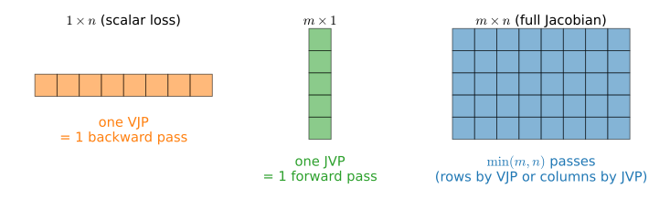
A network has millions of parameters and one loss, so reverse mode wins by a factor of the parameter count: millions. We will count the passes with our own two engines once both are built. The cheap-gradient principle (Baur and Strassen 1983; Griewank and Walther 2008) names the phenomenon: a scalar’s gradient costs a small constant multiple of one function evaluation, regardless of parameter count, and that is what makes training deep networks computationally feasible. This is backpropagation (Linnainmaa 1970; Speelpenning 1980; Rumelhart et al. 1986): the algorithm of Section 25.2 is reverse-mode AD, and the rule we followed there, “keep \(\partial f\) in the numerator”, is now rigorous.
25.3.4.2 The Tape: Record Forward, Replay Backward
Reverse mode cannot be done by a value-carrying algebra like dual numbers, because the multiplications run opposite to the program’s execution: we need each operation’s local Jacobian after the forward pass has finished. So we record the computation as it runs, and then walk the record backward. The record is called the Wengert list or tape, after the forward-mode paper (Wengert 1964) that introduced the list of elementary operations; running it backward is the later, reverse-mode idea (Linnainmaa 1970). The forward pass builds a directed acyclic graph of elementary operations and stashes the values needed for each local derivative; the backward pass seeds the output adjoint (the running \(\partial L/\partial\cdot\)) and pushes it through each recorded operation’s VJP, accumulating contributions where a value feeds several consumers. Figure 25.3.3 contrasts the two sweeps.
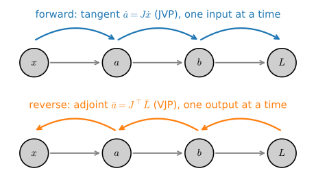
A tiny tape makes this concrete. We record each operation as a node holding its value and a backward closure that, given the adjoint of the node’s output, increments the adjoints of its inputs by the appropriate VJP. Replaying the tape in reverse and seeding the final adjoint with \(1\) leaves \(\partial L/\partial\cdot\) in every input’s adjoint slot.
class Var:
    """A scalar node on the autodiff tape; .grad accumulates the adjoint."""
    def __init__(self, value, parents=(), backward=lambda g: None):
        self.value = value
        self.grad = 0.0
        self._parents = parents                     # nodes this one depends on
        self._backward = backward                   # pushes adjoint to parents
    def __add__(self, o):
        o = o if isinstance(o, Var) else Var(o)
        out = Var(self.value + o.value, (self, o))
        def back(g):                                # d(a+b) = 1*g to each parent
            self.grad += g; o.grad += g
        out._backward = back
        return out
    __radd__ = __add__
    def __mul__(self, o):
        o = o if isinstance(o, Var) else Var(o)
        out = Var(self.value * o.value, (self, o))
        def back(g):                                # product rule, reversed
            self.grad += o.value * g; o.grad += self.value * g
        out._backward = back
        return out
    __rmul__ = __mul__

def backprop(node):
    """Topologically sort the tape and replay it backward from `node`."""
    order, seen = [], set()
    def visit(v):
        if v not in seen:
            seen.add(v)
            for p in v._parents:
                visit(p)
            order.append(v)
    visit(node)
    node.grad = 1.0                                 # seed the output adjoint
    for v in reversed(order):
        v._backward(v.grad)
We differentiate an expression with the same diamond-reuse structure that made the backward sweep of Section 25.2 efficient, and check the tape’s gradients against the framework’s autograd. Take \(g(u,v)=r^2\) with the shared intermediate \(r=uv+u\) (in code, r = u*v + u followed by y = r*r). One forward pass records the tape, one backward pass yields both partials. Its graph, Figure 25.3.4, is not a chain but a diamond: \(u\) feeds both the product \(uv\) and the sum \(r\), and \(r\) feeds both arguments of the final multiplication. This reuse is exactly why the backward pass must visit nodes in reverse topological order (each node before the nodes it depends on, so that its adjoint is complete before it is pushed onward) and accumulate adjoints with += rather than overwrite them: when the node \(y=r\cdot r\) runs its backward step, it pushes the contribution \(\bar y\,r\) into r.grad twice, once per argument, so the adjoint \(\bar r = 2r\bar y\) arrives as a sum. A node’s adjoint is the sum of the contributions along every outgoing edge, the chain rule’s “sum over paths” made operational.
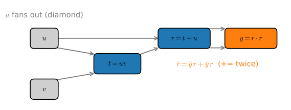
+=; here r.grad receives the contribution \(\bar y\,r\) twice, summing to \(\bar r=2r\bar y\).
u, v = Var(2.0), Var(-3.0)
r = u * v + u                                       # shared intermediate
y = r * r                                           # r feeds both arguments
backprop(y)
ut = torch.tensor(2.0, requires_grad=True)
vt = torch.tensor(-3.0, requires_grad=True)
rt = ut * vt + ut
(rt * rt).backward()                                # framework autograd
print('our tape   : dy/du = %.4f  dy/dv = %.4f' % (u.grad, v.grad))
print('torch      : dy/du = %.4f  dy/dv = %.4f' % (ut.grad, vt.grad))
our tape : dy/du = 16.0000 dy/dv = -16.0000
torch : dy/du = 16.0000 dy/dv = -16.0000u, v = Var(2.0), Var(-3.0)
r = u * v + u # shared intermediate
y = r * r # r feeds both arguments
backprop(y)
ut, vt = tf.Variable(2.0), tf.Variable(-3.0)
with tf.GradientTape() as tape: # framework autograd
rt = ut * vt + ut
yt = rt * rt
du, dv = tape.gradient(yt, [ut, vt])
print('our tape : dy/du = %.4f dy/dv = %.4f' % (u.grad, v.grad))
print('tensorflow : dy/du = %.4f dy/dv = %.4f' % (float(du), float(dv)))our tape : dy/du = 16.0000 dy/dv = -16.0000
tensorflow : dy/du = 16.0000 dy/dv = -16.0000u, v = Var(2.0), Var(-3.0)
r = u * v + u # shared intermediate
y = r * r # r feeds both arguments
backprop(y)
def g(u, v):
r = u * v + u
return r * r
du, dv = jax.grad(g, argnums=(0, 1))(2.0, -3.0) # framework autograd
print('our tape : dy/du = %.4f dy/dv = %.4f' % (u.grad, v.grad))
print('jax : dy/du = %.4f dy/dv = %.4f' % (float(du), float(dv)))our tape : dy/du = 16.0000 dy/dv = -16.0000
jax : dy/du = 16.0000 dy/dv = -16.0000u, v = Var(2.0), Var(-3.0)
r = u * v + u # shared intermediate
y = r * r # r feeds both arguments
backprop(y)
um, vm = mnp.array(2.0), mnp.array(-3.0)
um.attach_grad(); vm.attach_grad()
with autograd.record(): # framework autograd
rm = um * vm + um
ym = rm * rm
ym.backward()
print('our tape : dy/du = %.4f dy/dv = %.4f' % (u.grad, v.grad))
print('mxnet : dy/du = %.4f dy/dv = %.4f' % (float(um.grad), float(vm.grad)))our tape : dy/du = 16.0000 dy/dv = -16.0000
mxnet : dy/du = 16.0000 dy/dv = -16.0000Our thirty-line tape reproduces the framework’s gradients exactly. The real systems generalize it in three ways that do not change the principle: the nodes hold tensors rather than scalars, so each _backward is a VJP (a matrix operation, e.g. the \(\mathbf x^\top\) in Equation 25.3.6) rather than a scalar multiply; the primitive set is large (every differentiable op ships a VJP rule); and the graph is built either eagerly (PyTorch’s dynamic tape) or by tracing (JAX, TensorFlow). The underlying procedure is the same: record the forward computation, seed the output adjoint, and replay the graph backward while accumulating VJPs.
25.3.4.3 The Cost Asymmetry, Counted
The two implementations allow a direct comparison of pass counts. Take a scalar function of \(n=200\) inputs, built from nothing but the additions and multiplications both engines support. Forward mode must run one pass per input direction to assemble the gradient (a \(1\times n\) Jacobian, column by column); the tape runs one backward sweep.
n = 200
def f(xs):                       # f: R^n -> R, from + and * alone
    total = 0.0
    for x in xs:
        total = total + x * x
    return total * total         # (sum of squares)^2

xs0 = [0.01 * (j + 1) for j in range(n)]
passes, grad_fwd = 0, []
for j in range(n):               # forward mode: one pass per input direction
    duals = [Dual(x, 1.0 if k == j else 0.0) for k, x in enumerate(xs0)]
    grad_fwd.append(f(duals).b)
    passes += 1

xs = [Var(x) for x in xs0]       # reverse mode: one recorded forward pass...
backprop(f(xs))                  # ...and one backward sweep for all n partials
grad_rev = [x.grad for x in xs]

gap = max(abs(a - b) for a, b in zip(grad_fwd, grad_rev))
print(f'forward mode : {passes} passes (one per input)')
print(f'reverse mode : 1 backward sweep for all {n} partials')
print(f'max |forward - reverse| over the gradient: {gap:.1e}')
forward mode : 200 passes (one per input)
reverse mode : 1 backward sweep for all 200 partials
max |forward - reverse| over the gradient: 0.0e+00The two gradients agree to machine precision, but the pass counts differ by a factor of \(n\): \(200\) forward passes against one backward sweep, which is the loop structure itself. Each forward-mode pass costs about one evaluation of \(f\), and the tape’s recorded forward pass plus backward sweep costs a small constant multiple of one, so the work ratio is \(\Theta(n)\), i.e. proportional to \(n\) up to a constant factor. Nothing about the ratio is special to \(200\): replace it by the \(10^8\) parameters of a modern network and this factor is the “factor of millions” claimed above, which is why no framework computes training gradients in forward mode.
25.3.4.4 Jacobian Products Without Explicit Jacobians
The two engines above expose exactly two products, the forward-mode JVP \(\mathbf J\mathbf v\) and the reverse-mode VJP \(\mathbf u^\top\mathbf J\), and every quantity a training loop needs is built by composing those, never by materializing \(\mathbf J\). This is deliberate. Writing down a dense \(m\times n\) Jacobian costs \(\min(m,n)\) passes (one per column via JVP, or one per row via VJP) plus \(\Theta(mn)\) storage, while the thing you actually want (a gradient \(\mathbf u^\top\mathbf J\), a directional derivative \(\mathbf J\mathbf v\), a sequence of these through a deep composition) costs a single pass and never holds more than a vector. Autograd systems therefore expose the JVP and the VJP as their primitives and treat the full Jacobian as a rare, opt-in convenience. Even that convenience is built from the same parts: a Jacobian, when one is truly needed, is assembled by batching VJPs over the \(m\) output directions (rows) or JVPs over the \(n\) input directions (columns), and a Hessian by the forward-over-reverse composition of the next subsection, when \(n\) is small enough to afford one. If you find yourself assembling a Jacobian, you have almost certainly written down a matrix you could have multiplied through.
25.3.4.5 Hessian-Vector Products: One Order Up
The same approach applies one derivative order higher. Second-order optimizers and curvature diagnostics do not need the full Hessian \(\mathbf H=\nabla^2 L\), an \(n\times n\) object, hopeless to even store for \(n\) in the millions. Newton’s method, the conjugate-gradient (CG) method, and Gauss–Newton (Nocedal and Wright 2006) (see Chapter 26) all need only the Hessian–vector product \(\mathbf H\mathbf v\): the action of curvature in a single direction, e.g. one matrix-vector multiply inside a CG iteration. CG is an iterative linear-system solver that touches its matrix only through matrix-vector products, and Gauss–Newton approximates the Hessian by a product of first-derivative Jacobians. Pearlmutter’s trick (Pearlmutter 1994) obtains that product without forming \(\mathbf H\) by composing the two modes. Since \(\mathbf H = \nabla^2 L\) is the Jacobian of the gradient map \(\nabla L\), the Hessian–vector product is a directional derivative of the gradient,
\[ \mathbf H\mathbf v = \mathbf J_{\nabla L}\,\mathbf v = \left.\frac{d}{ds}\right|_{s=0}\nabla L(\mathbf x + s\mathbf v), \tag{25.3.11}\]
so we push the tangent \(\mathbf v\) through the gradient computation in forward over reverse: a forward-mode JVP applied to the reverse-mode gradient. The cost is a small constant multiple of one gradient evaluation: curvature in one chosen direction without \(n\) separate gradient evaluations (Baydin et al. 2018). Its absolute work still scales with the computation of \(L\) and therefore usually with the problem size. In terms of our toy engines, layering a Dual seed over the reverse-mode Var tape is exactly this forward-over-reverse construction. It is what makes Newton and conjugate-gradient methods and the curvature analysis of Chapter 29 tractable at scale.
The recipe is short enough to show whole. For the quadratic \(L(\mathbf x)=\tfrac12\mathbf x^\top\mathbf A\mathbf x\) with symmetric \(\mathbf A\), the gradient is \(\mathbf A\mathbf x\) and the Hessian is \(\mathbf A\) itself, so the correct answer is known in advance: \(\mathbf H\mathbf v = \mathbf A\mathbf v\). No \(2\times2\) matrix of second derivatives is ever assembled below; only the gradient map appears, differentiated once in the direction \(\mathbf v\).
# Hv for L(x) = x^T A x / 2, where H = A exactly
A = torch.tensor([[3.0, 1.0], [1.0, 2.0]])
L = lambda x: 0.5 * x @ A @ x
x, v = torch.tensor([1.0, -2.0]), torch.tensor([1.0, 0.5])
_, Hv = torch.func.jvp(torch.func.grad(L), (x,), (v,))  # forward over reverse
print('forward-over-reverse Hv:', Hv)
print('A v                    :', A @ v)
forward-over-reverse Hv: tensor([3.5000, 2.0000])
A v : tensor([3.5000, 2.0000])# Hv for L(x) = x^T A x / 2, where H = A exactly (tape over tape:
# reverse-over-reverse, TensorFlow's standard HVP construction)
A = tf.constant([[3.0, 1.0], [1.0, 2.0]])
x = tf.Variable([1.0, -2.0])
v = tf.constant([1.0, 0.5])
with tf.GradientTape() as outer:
with tf.GradientTape() as inner:
L = 0.5 * tf.tensordot(x, tf.linalg.matvec(A, x), 1)
g = inner.gradient(L, x)
gv = tf.tensordot(g, v, 1) # <grad L, v>, then one more grad
Hv = outer.gradient(gv, x)
print('reverse-over-reverse Hv:', Hv.numpy())
print('A v :', tf.linalg.matvec(A, v).numpy())reverse-over-reverse Hv: [3.5 2. ]
A v : [3.5 2. ]# Hv for L(x) = x^T A x / 2, where H = A exactly
A = jnp.array([[3.0, 1.0], [1.0, 2.0]])
L = lambda x: 0.5 * x @ A @ x
x, v = jnp.array([1.0, -2.0]), jnp.array([1.0, 0.5])
_, Hv = jax.jvp(jax.grad(L), (x,), (v,)) # forward over reverse
print('forward-over-reverse Hv:', Hv)
print('A v :', A @ v)forward-over-reverse Hv: [3.5 2. ]
A v : [3.5 2. ]# Hv for L(x) = x^T A x / 2, where H = A exactly. MXNet cannot tape its own
# backward pass, so we use eq_mdl-hvp directly: Hv is the directional
# derivative of the gradient map, here by a central difference
A = mnp.array([[3.0, 1.0], [1.0, 2.0]])
def grad_L(x):
x = x.copy()
x.attach_grad()
with autograd.record():
L = 0.5 * mnp.dot(x, mnp.dot(A, x))
L.backward()
return x.grad
x, v = mnp.array([1.0, -2.0]), mnp.array([1.0, 0.5])
h = 1e-4
Hv = (grad_L(x + h * v) - grad_L(x - h * v)) / (2 * h)
print('directional-derivative Hv:', Hv)
print('A v :', mnp.dot(A, v))directional-derivative Hv: [3.4993887 2.0003319]
A v : [3.5 2. ]The printed product equals \(\mathbf A\mathbf v\) to the digit. Exercise 7 works through the analytic claim and contrasts forward-over-reverse with the double-backward (reverse-over-reverse) alternative.
25.3.4.6 Differentiating Through Equations
So far we have differentiated an explicit program recorded on a tape. Some useful outputs in machine learning are defined implicitly, as the solution of an equation: the fixed point a solver converges to, the equilibrium of a physical model, the argmin of an inner optimization. Suppose \(\mathbf x^\star(\boldsymbol\theta)\) is defined by the condition
\[ \mathbf g\bigl(\mathbf x^\star(\boldsymbol\theta),\,\boldsymbol\theta\bigr) = \mathbf 0, \]
and we want \(\partial\mathbf x^\star/\partial\boldsymbol\theta\), say to train \(\boldsymbol\theta\) by gradient descent through the solver. Taping the solver’s dozens of iterations works but is wasteful and fragile. The implicit function theorem (Rudin 1976), which we use without proof, says we never have to: if \(\mathbf g\) is continuously differentiable and the Jacobian \(\partial\mathbf g/\partial\mathbf x\) is invertible at the solution, then \(\mathbf x^\star(\boldsymbol\theta)\) is locally a differentiable function of \(\boldsymbol\theta\), and differentiating the identity \(\mathbf g(\mathbf x^\star(\boldsymbol\theta),\boldsymbol\theta)\equiv\mathbf 0\) by the chain rule Equation 25.3.3 gives \(\frac{\partial\mathbf g}{\partial\mathbf x}\frac{\partial\mathbf x^\star}{\partial\boldsymbol\theta} +\frac{\partial\mathbf g}{\partial\boldsymbol\theta}=\mathbf 0\), hence
\[ \frac{\partial\mathbf x^\star}{\partial\boldsymbol\theta} = -\Bigl(\frac{\partial\mathbf g}{\partial\mathbf x}\Bigr)^{\!-1} \frac{\partial\mathbf g}{\partial\boldsymbol\theta}. \tag{25.3.12}\]
Both Jacobians on the right are evaluated at the solution only: the gradient of an implicitly defined output costs one linear solve, no matter how many iterations the solver ran. The “never form the Jacobian” discipline applies verbatim: a VJP \(\mathbf u^\top\partial\mathbf x^\star/\partial\boldsymbol\theta\) needs only one linear solve against \((\partial\mathbf g/\partial\mathbf x)^\top\), which is exactly the adjoint method that Section 29.1 uses to backpropagate through ODE solvers. Deep equilibrium models (Bai et al. 2019) make this the whole network: a layer’s output is the fixed point \(\mathbf x^\star=\mathbf f(\mathbf x^\star,\boldsymbol\theta)\), trained through Equation 25.3.12 alone, and bilevel problems such as hyperparameter optimization differentiate through an inner argmin the same way. The next cell verifies Equation 25.3.12 on a \(2\times2\) nonlinear system, against a finite difference of the solver’s output.
# Implicit gradient dx*/dtheta = -(dg/dx)^{-1} dg/dtheta on a 2x2 system,
# checked against a finite difference of the solver output
def g(x, th):                        # g(x, theta) = 0 defines x*(theta)
    return np.array([x[0]**2 + th * x[1] - 2, x[0] * x[1] + th - 1])

def dg_dx(x, th):                    # Jacobian in x, evaluated at (x, th)
    return np.array([[2 * x[0], th], [x[1], x[0]]])

def solve(th):                       # Newton iteration, from a fixed start
    x = np.array([1.0, 1.0])
    for _ in range(20):
        x = x - np.linalg.solve(dg_dx(x, th), g(x, th))
    return x

th, h = 0.3, 1e-6
xs = solve(th)
dg_dth = np.array([xs[1], 1.0])      # dg/dtheta at the solution
implicit = -np.linalg.solve(dg_dx(xs, th), dg_dth)
fd = (solve(th + h) - solve(th - h)) / (2 * h)
print('implicit-function gradient:', implicit.round(8))
print('finite-difference check   :', fd.round(8))
implicit-function gradient: [-0.11311451 -0.69322129]
finite-difference check : [-0.11311451 -0.69322129]The two vectors agree to the precision the finite difference allows. Note what the implicit route never touched: the twenty Newton iterations inside solve. Only the residual’s two Jacobians at the converged point enter Equation 25.3.12: the equation, not the algorithm that solved it, carries the derivative.
25.3.4.7 The Memory Trade-off and Checkpointing
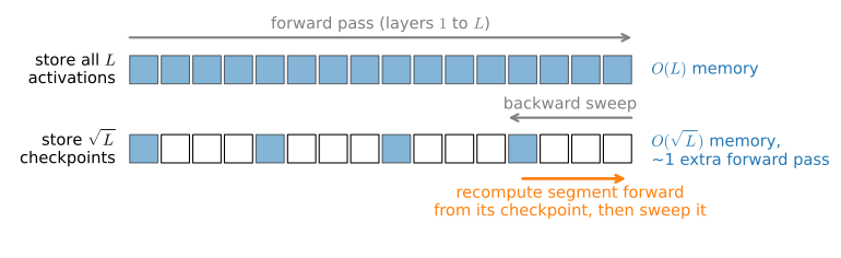
One cost is now visible. Reverse mode must store the forward intermediates (the values on the tape) until the backward pass consumes them, so its memory grows linearly with the length \(L\) of the computation, whereas forward mode keeps only the current value and tangent. For a deep network this \(O(L)\) activation memory is often the binding constraint on batch size and depth. Gradient checkpointing (Chen et al. 2016) buys it back: store only \(O(\sqrt L)\) of the intermediates and recompute the rest on the fly during the backward pass, turning \(O(L)\) memory into \(O(\sqrt L)\) at the cost of roughly one extra forward pass; Figure 25.3.5 draws the schedule. The trade-off can be pushed much further: Griewank’s treeverse algorithm (Griewank 1992) checkpoints recursively to reach \(O(\log L)\) memory, at the price of \(O(L\log L)\) recomputation, provably optimal among checkpointing schedules with the given snapshot budget. Forward and reverse modes, mixed modes, and checkpointing are treated in full in Griewank and Walther’s monograph Evaluating Derivatives (Griewank and Walther 2008) and in the survey (Baydin et al. 2018); the same reverse-mode tape returns as the adjoint method for differentiating through ODE solvers in Chapter 29.
25.3.5 Summary
- The Jacobian \(\mathbf J_{\mathbf f}\in\mathbb R^{m\times n}\) is the best local linear approximation of a vector-valued \(\mathbf f\): \(\mathbf f(\mathbf x+\boldsymbol\delta)\approx\mathbf f(\mathbf x)+\mathbf J\boldsymbol\delta\), with \([\mathbf J]_{ij}=\partial f_i/\partial x_j\). The row gradient (\(m=1\)) and the Hessian (Jacobian of \(\nabla f\)) are special cases.
- The chain rule in matrix form is Jacobian composition \(\mathbf J_{\mathbf g\circ\mathbf f}=\mathbf J_{\mathbf g}\mathbf J_{\mathbf f}\), so a depth-\(L\) network’s derivative is the matrix product \(\mathbf J_L\cdots\mathbf J_1\). Different associations of this product give forward- and reverse-mode AD.
- Layout conventions (numerator vs denominator) differ by a transpose; we use numerator layout for Jacobians and denominator (column) layout for gradients.
- The recurring DL identities all follow from differentiating one component and reassembling, not from a table: \(\nabla\,\mathbf a^\top\mathbf x=\mathbf a\), \(\nabla\,\mathbf x^\top\mathbf A\mathbf x=(\mathbf A+\mathbf A^\top)\mathbf x\), the rank-one \(\nabla_{\mathbf W}\|\mathbf W\mathbf x-\mathbf y\|^2=2(\mathbf W\mathbf x-\mathbf y)\mathbf x^\top\), and the softmax–cross-entropy logit gradient \(\mathbf p-\mathbf y\).
- Forward-mode AD carries a derivative via dual numbers (\(\varepsilon^2=0\)); one pass computes a Jacobian–vector product, a linear combination of columns (one literal column for a coordinate seed), so it is cheap for tall Jacobians.
- Reverse-mode AD records a tape and replays it backward, computing a vector–Jacobian product, a linear combination of rows (one literal row for a coordinate seed). Because a loss is scalar, backpropagation is reverse-mode AD: one backward sweep yields the gradient with respect to every parameter at a small constant multiple of one forward evaluation, at the price of storing the forward intermediates. The number of sweeps does not grow with \(n\); the cost of each sweep still follows the cost of the primal computation.
- Automatic differentiation composes JVPs and VJPs without usually forming the full Jacobian; a dense \(m\times n\) Jacobian costs \(\min(m,n)\) passes and is almost always avoidable. One order up, the Hessian–vector product \(\mathbf H\mathbf v\) comes from forward-over-reverse (Pearlmutter’s trick) at the cost of one extra gradient: curvature without forming \(\mathbf H\), which is what makes Newton/CG methods scale. The \(O(L)\) activation memory of the tape can be traded down to \(O(\sqrt L)\) by gradient checkpointing at roughly one extra forward pass.
- Implicitly defined outputs need no tape through the solver: if \(\mathbf g(\mathbf x^\star,\boldsymbol\theta)=\mathbf 0\), the implicit function theorem gives \(\partial\mathbf x^\star/\partial\boldsymbol\theta =-(\partial\mathbf g/\partial\mathbf x)^{-1}\partial\mathbf g/\partial\boldsymbol\theta\) from the Jacobians at the solution alone: one linear solve per gradient, the seed of the adjoint method, deep equilibrium models, and bilevel optimization.
25.3.6 Exercises
- Compute the Jacobian of \(\mathbf f(x,y)=(x^2y,\ \sin(x+y))\) and verify the linear approximation \(\mathbf f(\mathbf x+\boldsymbol\delta)\approx\mathbf f(\mathbf x)+\mathbf J\boldsymbol\delta\) at \((1,0)\) against a finite difference. By how much does the error shrink when you halve \(\boldsymbol\delta\)?
- Show \(\nabla_{\mathbf x}\|\mathbf A\mathbf x-\mathbf b\|_2^2=2\mathbf A^\top(\mathbf A\mathbf x-\mathbf b)\) two ways: by an index/Einstein-notation derivation, and by the scalar-collapse heuristic (guess from \(\frac{d}{dx}(ax-b)^2\), then fix the shapes with transposes).
- For a scalar loss with \(n=10^6\) parameters, how many passes does forward mode need to assemble the full gradient, and how many does reverse mode need? Explain via JVPs versus VJPs.
- Extend the
Dualclass with a__pow__(or alog) method and use it to differentiate \(f(x)=\log(1+x^2)\) at \(x=2\); check against the analytic derivative. Which rule from the proof of Equation 25.3.10 does each new method encode? - Add a new primitive (e.g. \(\exp\) or \(\sin\)) to the reverse-mode
Var/backproptape, give it the correct_backward, and verify a gradient against a framework’s autograd. - Derive the softmax Jacobian Equation 25.3.7 from the quotient rule, then re-derive the logit gradient \(\mathbf p-\mathbf y\) and explain why fusing softmax with cross-entropy is numerically preferable to composing them.
- Hessian–vector product. For \(L(\mathbf x)=\tfrac12\mathbf x^\top\mathbf A\mathbf x\) with symmetric \(\mathbf A\), show analytically that \(\nabla L=\mathbf A\mathbf x\) and hence \(\mathbf H\mathbf v=\mathbf A\mathbf v\). Then implement the forward-over-reverse recipe of Equation 25.3.11 for a general scalar \(L\) using a framework’s autograd (a forward-mode JVP pushed through the reverse-mode gradient: in PyTorch,
torch.func.jvp(torch.func.grad(L), (x,), (v,)); in JAX,jax.jvp(jax.grad(L), (x,), (v,))) and confirm it returns \(\mathbf A\mathbf v\) without ever building the \(n\times n\) matrix \(\mathbf H\). PyTorch’s classic double-backward alternative (differentiate \(\langle\nabla L,\mathbf v\rangle\) once more, viatorch.autograd.grad(L, x, create_graph=True)) computes the same product as reverse-over-reverse; it works, but it tapes the backward pass itself, so it costs somewhat more time and memory than forward-over-reverse. - Gradient of the log-absolute-determinant. For a real invertible \(\mathbf A\), show that \(\nabla_{\mathbf A}\log|\det\mathbf A|=\mathbf A^{-\top}\). (If \(\det\mathbf A>0\), this is also the gradient of \(\log\det\mathbf A\).) Hint: perturb one entry at a time: with \(\mathbf E=\mathbf e_a\mathbf e_b^\top\), expand \(\det(\mathbf A+\varepsilon\mathbf E)
=\det(\mathbf A)\det(\mathbf I+\varepsilon\mathbf A^{-1}\mathbf E)
\approx\det(\mathbf A)\,\bigl(1+\varepsilon\operatorname{tr}(\mathbf A^{-1}\mathbf E)\bigr)\) and read off the \((a,b)\) partial; equivalently, apply Jacobi’s formula \(\tfrac{d}{dt}\det\mathbf A(t)=\det\mathbf A(t)\,
\operatorname{tr}\bigl(\mathbf A(t)^{-1}\tfrac{d\mathbf A}{dt}\bigr)\). This identity is what makes the \(\log|\det\mathbf J|\) term of the change-of-variables formula for densities (Section 27.1) trainable by gradient descent; normalizing flows, generative models built from invertible maps and trained on exactly this log-likelihood (Section 29.4.3), depend on it. Verify it numerically by differentiating the log-absolute-determinant of a random invertible \(3\times3\) matrix (use a
slogdet-style routine) with a framework’s autograd and comparing against \(\mathbf A^{-\top}\). - Attention Jacobians. In self-attention (Section 10.2), softmax is applied row-wise to the score matrix \(\mathbf S=\mathbf Q\mathbf K^\top/\sqrt d\), giving attention weights \(\mathbf P\) with rows \(\mathbf p_i=\operatorname{softmax}(\mathbf s_i)\). Show that the Jacobian of the attention weights with respect to the scores is block-diagonal: row \(i\) of \(\mathbf P\) depends only on row \(i\) of \(\mathbf S\), and each block is exactly the per-row softmax Jacobian \(\operatorname{diag}(\mathbf p_i)-\mathbf p_i\mathbf p_i^\top\) of
Equation 25.3.7. Then push one step further down the chain: differentiating the scores \(\mathbf s_i=\mathbf K\mathbf q_i/\sqrt d\) with respect to the query \(\mathbf q_i\) contributes the Jacobian \(\mathbf K/\sqrt d\), so \(\partial\mathbf p_i/\partial\mathbf q_i
=\bigl(\operatorname{diag}(\mathbf p_i)-\mathbf p_i\mathbf p_i^\top\bigr)\mathbf K/\sqrt d\). Where does the temperature-like \(1/\sqrt d\) end up in the gradient, and what does it do to gradient magnitudes as \(d\) grows? Verify the block-diagonal structure numerically with a framework’s
jacobianon a \(3\times3\) score matrix.