import torch
from torch import nn5.2 Parameters, State, and Memory
A model’s state includes the tensors updated by the optimizer and the persistent tensors used by its computation. Checkpointing serializes this state, device placement moves it, and fine-tuning selects which parts to update. Its size also determines a substantial fraction of training memory. This section explains how to access state, distinguish parameters from buffers, count its storage, tie parameters, and freeze selected components.
import os
os.environ['TF_CPP_MIN_LOG_LEVEL'] = '2'
import tensorflow as tf
import jax
from jax import numpy as jnp
from flax import nnx
import optaximport os
from mxnet import autograd, gluon, np, npx
from mxnet.gluon import nn
npx.set_np()5.2.1 Accessing Parameters
Our specimen is the residual MLP of Section 5.1, redefined here so this section stands on its own: an input layer, a stack of residual blocks, and an output head.
class ResidualBlock(nn.Module):
    def __init__(self, d):
        super().__init__()
        self.body = nn.Sequential(nn.Linear(d, d), nn.ReLU(), nn.Linear(d, d))

    def forward(self, X):
        return X + self.body(X)

torch.manual_seed(42)
net = nn.Sequential(nn.Linear(20, 64), ResidualBlock(64),
                    ResidualBlock(64), nn.Linear(64, 10))
X = torch.randn(2, 20)
net(X).shape
torch.Size([2, 10])class ResidualBlock(tf.keras.layers.Layer):
def __init__(self, d):
super().__init__()
self.body = tf.keras.Sequential([
tf.keras.layers.Dense(d), tf.keras.layers.ReLU(),
tf.keras.layers.Dense(d)])
def call(self, X):
return X + self.body(X)
tf.keras.utils.set_random_seed(42)
net = tf.keras.Sequential([tf.keras.layers.Dense(64), ResidualBlock(64),
ResidualBlock(64), tf.keras.layers.Dense(10)])
X = tf.random.normal((2, 20))
net(X).shapeTensorShape([2, 10])class ResidualBlock(nnx.Module):
def __init__(self, d, rngs):
self.body = nnx.Sequential(
nnx.Linear(d, d, rngs=rngs), nnx.relu,
nnx.Linear(d, d, rngs=rngs))
def __call__(self, X):
return X + self.body(X)
rngs = nnx.Rngs(42)
net = nnx.Sequential(nnx.Linear(20, 64, rngs=rngs),
ResidualBlock(64, rngs), ResidualBlock(64, rngs),
nnx.Linear(64, 10, rngs=rngs))
X = jax.random.normal(jax.random.key(0), (2, 20))
net(X).shape(2, 10)class ResidualBlock(nn.Block):
def __init__(self, d):
super().__init__()
self.body = nn.Sequential()
self.body.add(nn.Dense(d, activation='relu'), nn.Dense(d))
def forward(self, X):
return X + self.body(X)
np.random.seed(42)
net = nn.Sequential()
net.add(nn.Dense(64), ResidualBlock(64), ResidualBlock(64), nn.Dense(10))
net.initialize()
X = np.random.uniform(size=(2, 20))
net(X).shape(2, 10)A model built from modules is a tree, and its parameters are the leaves. To reach one leaf, walk the tree: indexing into a Sequential selects a child, attribute access selects within it. net[3] is the output layer; its bias is an nn.Parameter, a tensor that announces itself to the module system as trainable.
A model built from layers is a tree, and its parameters are the leaves. To reach one leaf, walk the tree: net.layers lists a model’s children, attribute access selects within a layer. net.layers[3] is the output layer; its bias is a Variable the layer created through add_weight, announcing itself to Keras as trainable.
A model built from NNX modules is an object graph, and its parameters are nnx.Param variables owned by the layers. To reach one, follow ordinary attributes and container indices. net.layers[3] is the output layer and its bias variable is marked trainable by its type.
A model built from blocks is a tree, and its parameters are the leaves. To reach one leaf, walk the tree: indexing into a Sequential selects a child, attribute access selects within it. net[3] is the output layer; its bias is a Parameter, an object that announces itself to the block system as state, bundling the tensor with its gradient buffer; .data() returns the tensor, and .shape reads through to it.
type(net[3].bias), net[3].bias.shape(torch.nn.parameter.Parameter, torch.Size([10]))type(net.layers[3].bias), net.layers[3].bias.shape(keras.src.backend.Variable, TensorShape([10]))bias = net.layers[3].bias
type(bias), bias.shape(flax.nnx.variablelib.Param, (10,))type(net[3].bias), net[3].bias.shape(mxnet.gluon.parameter.Parameter, (10,))The same path syntax reaches arbitrarily deep. The first linear layer inside the first residual block sits three levels down:
net[1].body[0].weight.shapetorch.Size([64, 64])net.layers[1].body.layers[0].kernel.shapeTensorShape([64, 64])net.layers[1].body.layers[0].kernel.shape(64, 64)net[1].body[0].weight.shape(64, 64)Each parameter also carries its gradient. We have not run backpropagation on this model yet, so there is nothing to see:
Gradients are not stored on variables. A tf.GradientTape records the forward pass, and its gradient method returns the gradients as a second list, parallel to the variables you differentiate with respect to:
Gradients are not stored on parameters. nnx.grad returns a second state tree with the same parameter paths, one gradient leaf per parameter:
The gradient is the second array a Parameter carries: .data() returns the value and .grad() its gradient buffer. gluon allocates the buffer alongside the data at initialization time, so before any backpropagation it holds zeros:
net[3].weight.grad is NoneTruewith tf.GradientTape() as tape:
loss = tf.reduce_sum(net(X))
grads = tape.gradient(loss, net.trainable_weights)
len(grads) == len(net.trainable_weights)Trueparams = nnx.state(net, nnx.Param)
grads = nnx.grad(lambda model: model(X).sum())(net)
jax.tree_util.tree_structure(grads) == jax.tree_util.tree_structure(params)Truenet[3].bias.grad()array([0., 0., 0., 0., 0., 0., 0., 0., 0., 0.])Reaching parameters one path at a time is right for debugging a single layer. The optimizer, weight decay, and checkpointing instead need every leaf, and named_parameters() provides exactly that: a traversal of the whole tree that yields each parameter with its path as the name.
Reaching parameters one path at a time is right for debugging a single layer. The optimizer, weight decay, and checkpointing instead need every leaf, and net.weights provides exactly that: a traversal of the whole tree, one variable per leaf, each carrying its path as its name.
Reaching parameters one path at a time is right for debugging a single layer. The optimizer, weight decay, and checkpointing instead need every leaf, and nnx.state(net, nnx.Param) selects them. Its flat view yields each array together with the object-graph path that reaches it.
Reaching parameters one path at a time is right for debugging a single layer. The optimizer, weight decay, and checkpointing instead need every leaf, and collect_params() provides exactly that: a traversal of the whole tree that returns a dictionary of every parameter keyed by its path.
[(name, p.shape) for name, p in net.named_parameters()][('0.weight', torch.Size([64, 20])),
('0.bias', torch.Size([64])),
('1.body.0.weight', torch.Size([64, 64])),
('1.body.0.bias', torch.Size([64])),
('1.body.2.weight', torch.Size([64, 64])),
('1.body.2.bias', torch.Size([64])),
('2.body.0.weight', torch.Size([64, 64])),
('2.body.0.bias', torch.Size([64])),
('2.body.2.weight', torch.Size([64, 64])),
('2.body.2.bias', torch.Size([64])),
('3.weight', torch.Size([10, 64])),
('3.bias', torch.Size([10]))][(v.path, v.shape) for v in net.weights][('sequential_2/dense/kernel', TensorShape([20, 64])),
('sequential_2/dense/bias', TensorShape([64])),
('sequential_2/residual_block/sequential/dense_1/kernel',
TensorShape([64, 64])),
('sequential_2/residual_block/sequential/dense_1/bias', TensorShape([64])),
('sequential_2/residual_block/sequential/dense_2/kernel',
TensorShape([64, 64])),
('sequential_2/residual_block/sequential/dense_2/bias', TensorShape([64])),
('sequential_2/residual_block_1/sequential_1/dense_3/kernel',
TensorShape([64, 64])),
('sequential_2/residual_block_1/sequential_1/dense_3/bias',
TensorShape([64])),
('sequential_2/residual_block_1/sequential_1/dense_4/kernel',
TensorShape([64, 64])),
('sequential_2/residual_block_1/sequential_1/dense_4/bias',
TensorShape([64])),
('sequential_2/dense_5/kernel', TensorShape([64, 10])),
('sequential_2/dense_5/bias', TensorShape([10]))][(path, leaf.shape) for path, leaf in params.flat_state()][(('layers', 0, 'bias'), (64,)),
(('layers', 0, 'kernel'), (20, 64)),
(('layers', 1, 'body', 'layers', 0, 'bias'), (64,)),
(('layers', 1, 'body', 'layers', 0, 'kernel'), (64, 64)),
(('layers', 1, 'body', 'layers', 2, 'bias'), (64,)),
(('layers', 1, 'body', 'layers', 2, 'kernel'), (64, 64)),
(('layers', 2, 'body', 'layers', 0, 'bias'), (64,)),
(('layers', 2, 'body', 'layers', 0, 'kernel'), (64, 64)),
(('layers', 2, 'body', 'layers', 2, 'bias'), (64,)),
(('layers', 2, 'body', 'layers', 2, 'kernel'), (64, 64)),
(('layers', 3, 'bias'), (10,)),
(('layers', 3, 'kernel'), (64, 10))][(name, p.shape) for name, p in net.collect_params().items()][('0.weight', (64, 20)),
('0.bias', (64,)),
('1.body.0.weight', (64, 64)),
('1.body.0.bias', (64,)),
('1.body.1.weight', (64, 64)),
('1.body.1.bias', (64,)),
('2.body.0.weight', (64, 64)),
('2.body.0.bias', (64,)),
('2.body.1.weight', (64, 64)),
('2.body.1.bias', (64,)),
('3.weight', (10, 64)),
('3.bias', (10,))]Read one of the names closely. 1.body.0.weight means: child 1 of net (the first residual block), its submodule body, that module’s child 0, and finally the leaf weight. Names are paths, so they survive any amount of nesting, and they are exactly the keys of the model’s state_dict, the name-to-tensor mapping used for saving and loading (Section 5.6):
Read one of the paths closely. sequential_2/residual_block/sequential/dense_1/kernel means: inside the outer Sequential, its child residual_block (the first residual block), that block’s body (a Sequential of its own), the first Dense inside it, and finally the leaf kernel. The segments are layer names, assigned at construction: a default derived from the class, plus a counter that keeps names unique across the program (this is the third Sequential created, hence sequential_2). The paths expose ownership for inspection, but default names depend on construction history and are not an external identifier. Name layers explicitly when a tool must match paths across separately written programs; Keras checkpoints otherwise restore through the saved object topology and weight structure (Section 5.6). Keras splits the same list by trainability, and so far the split is trivial:
Read one of the paths closely. ('layers', 1, 'body', 'layers', 0, 'kernel') means: child 1 of net, the first residual block, its body, child 0 of that sequence, and finally its kernel. Paths survive arbitrary nesting. Filters select the kinds of state a consumer needs, while checkpoints can save the full state (Section 5.6):
Read one of the names closely. 1.body.0.weight means: child 1 of net (the first residual block), its submodule body, that block’s child 0, and finally the leaf weight. Names are paths, so they survive any amount of nesting, and they are exactly the names save_parameters writes and load_parameters expects (Section 5.6). Nor is there a separate list of trainable parameters: each Parameter carries a grad_req attribute that tells autograd whether to record a gradient for it, and so far every entry says 'write':
list(net.state_dict()) == [name for name, _ in net.named_parameters()]True[v.path for v in net.weights] == [v.path for v in net.trainable_weights]Truelist(params)['layers']params = net.collect_params()
[name for name, p in params.items() if p.grad_req == 'write'] == list(params)TrueOne tree, one naming scheme, and every consumer, whether optimizer, checkpoint, or debugger, walks it. The equality above holds for this model because all of its state happens to be trainable. That is not always so.
One tree, one naming scheme, and every consumer, whether optimizer, checkpoint, or debugger, walks it. The equality above holds for this model because all of its state happens to be trainable. That is not always so.
One tree, one naming scheme, and every consumer, whether optimizer, checkpoint, or debugger, walks it. This model has only nnx.Param state. That is not always so.
One dictionary, one naming scheme, and every consumer, whether optimizer, checkpoint, or debugger, walks it. The equality above holds for this model because all of its state happens to be trainable. That is not always so.
5.2.2 Parameters and Buffers
Some tensors must persist inside a model and follow it from device to device, yet should never receive a gradient. The canonical example is batch normalization (Ioffe and Szegedy 2015): each layer maintains a running mean and variance of its inputs, updated during the forward pass and used at prediction time. Those statistics must be saved with the model and must move to the GPU with it, but the optimizer has no business touching them. A precomputed positional table may be treated the same way. Other non-trained state has a different lifetime: a language model’s key–value cache belongs to one generation request, so it follows the computation device but should not be stored in a model checkpoint. Causal masks are often recomputed or registered as non-persistent state for the same reason.
PyTorch calls such tensors buffers, registered with register_buffer. The rule of thumb: make it a parameter if the optimizer should update it, a persistent buffer if checkpoints need it, and an explicit runtime input or cache if its lifetime is one request. Plain Python attributes hold reconstructible architecture data. Here is a module that standardizes its inputs with statistics computed once, ahead of time, from a reference sample:
Keras calls every registered tensor a weight and distinguishes by a per-variable flag: add_weight(trainable=False) creates a variable that is saved with the model but never handed to the optimizer, which is how BatchNormalization stores its running statistics. The rule of thumb: make it a trainable weight if the optimizer should update it, a non-trainable weight if it must persist in checkpoints, and an explicit runtime input or cache if its lifetime is one request. Plain Python attributes hold reconstructible architecture data. Here is a layer that standardizes its inputs with statistics computed once, ahead of time, from a reference sample:
NNX uses Variable subclasses to distinguish kinds of state. nnx.Param marks trainable state, nnx.BatchStat marks running statistics, and a custom subclass can mark another persistent buffer. Filters select which kinds an optimizer or checkpoint sees, so an ephemeral cache can remain outside the checkpoint filter or be passed explicitly. Here is a module that standardizes its inputs with statistics computed once from a reference sample:
gluon needs no second mechanism for such tensors: a Constant is a Parameter, one whose grad_req is hardwired to 'null'. Assigning one to an attribute registers it like any other parameter, so it appears in collect_params(), is saved with the model, and moves with it across devices; but autograd never records a gradient for it and the optimizer never touches it. The rule of thumb: make it a Parameter if the optimizer should update it, a Constant if checkpoints need it, and an explicit runtime input or cache if its lifetime is one request. Plain Python attributes hold reconstructible architecture data. Here is a block that standardizes its inputs with statistics computed once, ahead of time, from a reference sample:
class Whitener(nn.Module):
    def __init__(self, mean, std):
        super().__init__()
        self.register_buffer('mean', mean)
        self.register_buffer('std', std)
        self.out = nn.Linear(4, 2)

    def forward(self, X):
        return self.out((X - self.mean) / self.std)

sample = torch.randn(100, 4) * torch.arange(1., 5.)
whiten = Whitener(sample.mean(0), sample.std(0))
list(whiten.state_dict())
['mean', 'std', 'out.weight', 'out.bias']class Whitener(tf.keras.layers.Layer):
def __init__(self, mean, std):
super().__init__()
self.mean = self.add_weight(
shape=mean.shape, trainable=False, name='mean',
initializer=tf.keras.initializers.Constant(mean))
self.std = self.add_weight(
shape=std.shape, trainable=False, name='std',
initializer=tf.keras.initializers.Constant(std))
self.out = tf.keras.layers.Dense(2)
def call(self, X):
return self.out((X - self.mean) / self.std)
sample = tf.random.normal((100, 4)) * tf.range(1., 5.)
whiten = Whitener(tf.reduce_mean(sample, 0), tf.math.reduce_std(sample, 0))
_ = whiten(sample[:2]) # build the Dense layer
[v.path for v in whiten.weights]['whitener/mean',
'whitener/std',
'whitener/dense_6/kernel',
'whitener/dense_6/bias']class Buffer(nnx.Variable):
pass
class Whitener(nnx.Module):
def __init__(self, mean, std, rngs):
self.mean = Buffer(mean)
self.std = Buffer(std)
self.out = nnx.Linear(4, 2, rngs=rngs)
def __call__(self, X):
return self.out((X - self.mean) / self.std)
sample = jax.random.normal(jax.random.key(1), (100, 4)) * jnp.arange(1., 5.)
whiten = Whitener(sample.mean(0), sample.std(0), nnx.Rngs(2))
[(path, value.shape) for path, value in nnx.state(whiten).flat_state()][(('mean',), (4,)),
(('out', 'bias'), (2,)),
(('out', 'kernel'), (4, 2)),
(('std',), (4,))]class Whitener(nn.Block):
def __init__(self, mean, std):
super().__init__()
self.mean = gluon.Constant(mean)
self.std = gluon.Constant(std)
self.out = nn.Dense(2)
def forward(self, X):
return self.out((X - self.mean.data()) / self.std.data())
sample = np.random.normal(0, 1, (100, 4)) * np.arange(1., 5.)
whiten = Whitener(sample.mean(axis=0), sample.std(axis=0))
whiten.initialize()
whiten(sample[:2]) # build the deferred Dense layer
list(whiten.collect_params())['mean', 'std', 'out.weight', 'out.bias']The buffers appear in the state dict, so they are checkpointed alongside the weights. They do not appear among the parameters, so the optimizer never sees them:
All four variables are weights, so all four are checkpointed. The flag is what keeps the optimizer away from the statistics: a training step differentiates and updates trainable_weights, and the two constants sit in the other half of the split:
Both kinds belong to the object graph and can be checkpointed together. The optimizer selects nnx.Param, so it never sees the statistics.
The constants sit in the same dictionary as the weights, so they are checkpointed alongside them. What keeps the optimizer away is the grad_req on each entry:
[name for name, _ in whiten.named_parameters()]['out.weight', 'out.bias']([v.path for v in whiten.trainable_weights],
[v.path for v in whiten.non_trainable_weights])(['whitener/dense_6/kernel', 'whitener/dense_6/bias'],
['whitener/mean', 'whitener/std']){'params': list(nnx.state(whiten, nnx.Param)),
'buffers': list(nnx.state(whiten, Buffer))}{'params': ['out'], 'buffers': ['mean', 'std']}{name: p.grad_req for name, p in whiten.collect_params().items()}{'mean': 'null', 'std': 'null', 'out.weight': 'write', 'out.bias': 'write'}Registration is what makes the module system aware of a tensor. A tensor stored as a plain attribute is invisible to it: not saved, and not converted when the model moves. We can see this on the CPU by moving the module across dtypes, which uses the same machinery as moving across devices. The registered buffer converts; the plain attribute is left behind:
Registration through add_weight is what makes the layer aware of a tensor. A tensor stored as a plain attribute is invisible to it: not counted, not saved, and absent from every traversal. Attach one and the weights list does not grow:
Wrapping an array in a Variable makes it state. We can see the resulting tree operation on the CPU by splitting the graph, casting every state leaf, and merging a low-precision clone. The original model remains unchanged:
Registration is what makes the block aware of a tensor, and assignment only registers Parameters (a Constant is one) and child blocks. A raw array stored as a plain attribute is invisible: not saved, and not converted when the model moves. We can see this on the CPU by moving the block across dtypes, which uses the same machinery as moving across devices. The registered constant converts; the plain attribute is left behind:
whiten.note = torch.zeros(4)   # plain attribute: invisible to the module
whiten.to(torch.float64)
whiten.mean.dtype, whiten.note.dtype
(torch.float64, torch.float32)whiten.note = tf.zeros(4) # plain attribute: invisible to the layer
[v.path.split('/')[-1] for v in whiten.weights]['mean', 'std', 'kernel', 'bias']graph, state = nnx.split(whiten)
low = nnx.merge(graph, jax.tree.map(lambda x: x.astype(jnp.float16), state))
low.mean.dtype, whiten.mean.dtype(dtype('float16'), dtype('float32'))whiten.note = np.zeros(4) # plain attribute: invisible to the block
whiten.cast('float64')
whiten.mean.data().dtype, whiten.note.dtype(dtype('float64'), dtype('float32'))The same registration issue appears during device movement: a model works on the CPU, then crashes after .to('cuda') because an unregistered tensor stayed behind. On a machine with a GPU the following confirms that buffers move with the module:
Device placement works differently here: a TensorFlow variable’s device is decided when the variable is created, not by a later move. With a GPU visible, Keras creates variables on it by default, non-trainable weights included, and a tf.device scope overrides the choice. There is no .to() to forget, so an unregistered tensor cannot be left behind by .to(); the price is that relocating existing state means rebuilding it. Each variable reports its placement:
Device placement follows the same rule: jax.device_put moves a whole state tree, parameters and buffers alike. Updating the model with that tree moves all registered state. The same lines work on any host; on a machine with an accelerator, jax.devices()[0] is a GPU or TPU:
The same registration issue appears during device movement: a model works on the CPU, then crashes after reset_device(npx.gpu(0)) because an unregistered tensor stayed behind. On a machine with a GPU the following confirms that constants move with the block:
if torch.cuda.is_available():
    print('buffer lives on', whiten.to('cuda').mean.device)
else:
    print('no GPU here; on a CUDA machine, whiten.to("cuda") '
          'moves whiten.mean along with the parameters')
buffer lives on cuda:0whiten.mean.value.device # decided when the variable was created'/job:localhost/replica:0/task:0/device:GPU:0'moved = jax.device_put(nnx.state(whiten), jax.devices()[0])
nnx.update(whiten, moved)
whiten.mean.deviceCudaDevice(id=0)if npx.num_gpus() > 0:
whiten.reset_device(npx.gpu(0))
print('constant lives on', whiten.mean.data().device)
else:
print('no GPU here; on a CUDA machine, whiten.reset_device(npx.gpu(0)) '
'moves whiten.mean along with the parameters')constant lives on gpu(0)5.2.3 Counting Parameters, Counting Bytes
An initial memory estimate begins with persistent state per parameter: the weight, its gradient, and optimizer slots. For dense Adam with fp32 weights, gradients, and two fp32 running moments, the idealized calculation is:
| Training state | Precision | Bytes per parameter |
|---|---|---|
| Weights | fp32 | 4 |
| Gradients | fp32 | 4 |
| Adam first moment | fp32 | 4 |
| Adam second moment | fp32 | 4 |
| Total | 16 |
This 16-byte figure is a lower-bound accounting of persistent dense state. It excludes activations, temporary workspaces, allocator fragmentation, mixed-precision master copies, exponential moving averages, communication buffers, and changes from sharding. Section 5.7 measures total device allocation and peak memory directly.
n = sum(p.numel() for p in net.parameters())
weights, grads, adam_state = 4 * n, 4 * n, 8 * n   # bytes, all fp32
print(f'{n} parameters: {(weights + grads + adam_state) / 2**20:.2f} MiB '
      'for weights + gradients + Adam state')
18634 parameters: 0.28 MiB for weights + gradients + Adam staten = net.count_params()
weights = sum(int(tf.size(v)) * tf.as_dtype(v.dtype).size
for v in net.weights) # fp32: 4 bytes
grads, adam_state = weights, 2 * weights
print(f'{n} parameters: {(weights + grads + adam_state) / 2**20:.2f} MiB '
'for weights + gradients + Adam state')18634 parameters: 0.28 MiB for weights + gradients + Adam stateparams = nnx.state(net, nnx.Param)
leaves = jax.tree_util.tree_leaves(params)
n = sum(x.size for x in leaves)
weights = sum(x.size * x.dtype.itemsize for x in leaves) # fp32: 4 bytes
grads, adam_state = weights, 2 * weights
print(f'{n} parameters: {(weights + grads + adam_state) / 2**20:.2f} MiB '
'for weights + gradients + Adam state')18634 parameters: 0.28 MiB for weights + gradients + Adam stateparams = net.collect_params()
n = sum(p.data().size for p in params.values())
weights = sum(p.data().size * p.data().dtype.itemsize
for p in params.values()) # fp32: 4 bytes
grads, adam_state = weights, 2 * weights
print(f'{n} parameters: {(weights + grads + adam_state) / 2**20:.2f} MiB '
'for weights + gradients + Adam state')18634 parameters: 0.28 MiB for weights + gradients + Adam stateThe optimizer state is real memory, allocated tensor by tensor. After a single training step, Adam’s two moments together hold exactly two extra copies of the model:
adam = torch.optim.Adam(net.parameters())
net(X).sum().backward()
adam.step()
moments = sum(t.numel() for s in adam.state.values()
              for t in s.values() if torch.is_tensor(t) and t.ndim > 0)
moments == 2 * nTrueadam = tf.keras.optimizers.Adam()
adam.build(net.trainable_weights) # Keras allocates the moments here, up front
with tf.GradientTape() as tape:
loss = tf.reduce_sum(net(X))
adam.apply_gradients(zip(tape.gradient(loss, net.trainable_weights),
net.trainable_weights))
moments = sum(int(tf.size(v)) for v in adam.variables
if v.ndim > 0) # ndim 0 excludes the step count and learning rate
moments == 2 * nTrueoptimizer = nnx.Optimizer(net, optax.adam(1e-3), wrt=nnx.Param)
grads = nnx.grad(lambda model: model(X).sum())(net)
optimizer.update(net, grads)
moments = sum(x.size for x in jax.tree.leaves(optimizer.opt_state)
if hasattr(x, 'ndim') and x.ndim > 0)
moments == 2 * nTruetrainer = gluon.Trainer(net.collect_params(), 'adam')
with autograd.record():
loss = net(X).sum()
loss.backward()
trainer.step(batch_size=1) # the updater allocates the moments here
trainer.save_states('adam.states')
state_bytes = os.path.getsize('adam.states')
state_bytes, 8 * n(151114, 149072)gluon’s Trainer owns this state and offers no public traversal of it: the updater inside creates, at each parameter’s first update, two zero arrays shaped like the weight. What it does offer is save_states, which serializes exactly that state, so up to a sliver of packaging the file is Adam’s two moments: 8 bytes per parameter, two extra copies of the model.
For our little network the total is a third of a megabyte, which is why none of this mattered until now. Scale the same arithmetic to a 1-billion-parameter model and the standard fp32 Adam ledger gives a batch-independent floor: 4 GB for the weights alone and 16 GB for weights, gradients, and optimizer state, before storing a single activation (Section 9.6). Activations depend on batch size, sequence length, and architecture; they can exceed parameter state and are treated in Section 5.7.
Large models often train in mixed precision (Micikevicius et al. 2018), but storage policies differ. One implementation convention counts 18 bytes per parameter (fp32 master weights, an fp16 working copy, fp32 gradients, and two fp32 moments); the ZeRO paper counts 16 by keeping gradients in fp16 (Rajbhandari et al. 2020). Other bf16 and AMP stacks keep no separate working copy or choose another dtype for optimizer state. State the dtypes before quoting a multiplier. In the two conventions above, the fp32 Adam moments alone cost 8 bytes per parameter.
In gluon the fp32 master copy is one optimizer flag away: construct the Trainer with optimizer_params={'multi_precision': True} and, for every fp16 weight, the updater keeps an fp32 copy next to the two moments and applies updates to it. That is the master-weights term of the accounting above, 4 more bytes per parameter.
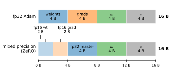
Figure 5.2.1 lays the two conventions side by side, byte for byte: the moments (right half of each bar) line up exactly, and the only disagreement is how the weights and gradients themselves are stored.
5.2.4 Tied Parameters
One tensor can serve several roles in a model. The standard example is the two ends of a language model. The input embedding is a \(|V| \times d\) table mapping each of \(|V|\) tokens to a \(d\)-dimensional vector; the output projection maps a \(d\)-dimensional hidden state to \(|V|\) logits, and its weight matrix has the same shape and an analogous meaning: one vector per token. Tying the two roles to a single tensor saves \(|V| \times d\) parameters. The cited studies also found lower language-model perplexity in their experimental settings (Press and Wolf 2017; Inan et al. 2017). The savings are large: in GPT-2 (Radford et al. 2019) the shared \(50257 \times 768\) matrix is about 38.6 million of the model’s 124 million parameters, roughly 31%.
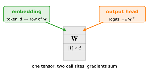
Figure 5.2.2 sketches the picture behind the two call sites.
A miniature version shows the mechanics. Tying is one assignment, and it is aliasing, not copying:
A miniature version shows the mechanics. Keras has no tying flag, so we say it in code: a small head layer that creates no variables of its own and instead multiplies by the transpose of the embedding table it is handed. One variable, two call sites:
A miniature version shows the mechanics. nnx.Embed provides attend, which multiplies a hidden state by the transpose of the embedding table, exactly the output projection. Calling it reuses the module’s one kernel, so the tying is visible in the state itself: no head matrix exists.
A miniature version shows the mechanics. gluon stores a Dense weight as (outputs, inputs), so the head’s weight has shape \((|V|, d)\): the embedding table’s shape exactly, no transpose required. Tying is share_parameters, which re-points the head’s 'weight' slot at the embedding’s Parameter, matched by name; it is aliasing, not copying:
class TinyLM(nn.Module):
    def __init__(self, vocab_size, d, tied=True):
        super().__init__()
        self.emb = nn.Embedding(vocab_size, d)
        self.body = nn.Linear(d, d)
        self.head = nn.Linear(d, vocab_size, bias=False)
        if tied:
            self.head.weight = self.emb.weight   # one tensor, two roles

    def forward(self, tokens):
        return self.head(torch.relu(self.body(self.emb(tokens))))

lm = TinyLM(vocab_size=100, d=16)
lm.head.weight is lm.emb.weightTrueclass TiedLMHead(tf.keras.layers.Layer):
def __init__(self, emb):
super().__init__()
self.emb = emb # reuse the embedding layer; create nothing
def call(self, h):
return tf.matmul(h, self.emb.embeddings, transpose_b=True)
class TinyLM(tf.keras.Model):
def __init__(self, vocab_size, d, tied=True):
super().__init__()
self.emb = tf.keras.layers.Embedding(vocab_size, d)
self.body = tf.keras.layers.Dense(d)
self.head = (TiedLMHead(self.emb) if tied else
tf.keras.layers.Dense(vocab_size, use_bias=False))
def call(self, tokens):
return self.head(tf.nn.relu(self.body(self.emb(tokens))))
lm = TinyLM(vocab_size=100, d=16)
tokens = tf.random.uniform((2, 8), 0, 100, dtype=tf.int32)
_ = lm(tokens) # build
[(v.path, tuple(v.shape)) for v in lm.weights][('tiny_lm/embedding/embeddings', (100, 16)),
('tiny_lm/dense_7/kernel', (16, 16)),
('tiny_lm/dense_7/bias', (16,))]class TinyLM(nnx.Module):
def __init__(self, vocab_size, d, tied=True, rngs=None):
rngs = nnx.Rngs(0) if rngs is None else rngs
self.tied = tied
self.emb = nnx.Embed(vocab_size, d, rngs=rngs)
self.body = nnx.Linear(d, d, rngs=rngs)
self.head = None if tied else nnx.Linear(
d, vocab_size, use_bias=False, rngs=rngs)
def __call__(self, tokens):
h = nnx.relu(self.body(self.emb(tokens)))
if self.tied:
return self.emb.attend(h) # the embedding table, used as the head
return self.head(h)
lm = TinyLM(vocab_size=100, d=16)
tokens = jax.random.randint(jax.random.key(1), (2, 8), 0, 100)
[(path, value.shape)
for path, value in nnx.state(lm, nnx.Param).flat_state()][(('body', 'bias'), (16,)),
(('body', 'kernel'), (16, 16)),
(('emb', 'embedding'), (100, 16))]class TinyLM(nn.Block):
def __init__(self, vocab_size, d):
super().__init__()
self.emb = nn.Embedding(vocab_size, d)
self.body = nn.Dense(d, flatten=False)
self.head = nn.Dense(vocab_size, use_bias=False, flatten=False)
def forward(self, tokens):
return self.head(npx.relu(self.body(self.emb(tokens))))
lm = TinyLM(vocab_size=100, d=16)
lm.initialize()
lm.head.share_parameters(lm.emb.collect_params()) # one tensor, two roles
tokens = np.random.randint(0, 100, (2, 8))
lm(tokens)
lm.head.weight is lm.emb.weightTrueThe module system understands the aliasing. Parameter traversal reports the shared tensor once, so the count below reflects the \(|V| \times d\) saving and the optimizer updates the tensor once per step:
Because the head created no variable, there is no aliasing bookkeeping to get right: the traversal reports the table once and no head matrix exists. The parameter count reflects the \(|V| \times d\) saving, and the optimizer updates the table once per step:
There is no aliasing bookkeeping to get right, because the state contains the table once. The parameter count reflects the \(|V| \times d\) saving, and an optimizer updates the table once per step:
The two blocks now hold one Parameter between them. collect_params() keeps both names pointing at it, so a naive sum over the dictionary would count the table twice; deduplicating by identity shows the \(|V| \times d\) saving. The Trainer deduplicates the same way internally and updates the table once per step:
untied = TinyLM(vocab_size=100, d=16, tied=False)
(sum(p.numel() for p in lm.parameters()),
 sum(p.numel() for p in untied.parameters()))
(1872, 3472)untied = TinyLM(vocab_size=100, d=16, tied=False)
_ = untied(tokens)
(lm.count_params(), untied.count_params())(1872, 3472)untied = TinyLM(vocab_size=100, d=16, tied=False)
(sum(x.size for x in jax.tree.leaves(nnx.state(lm, nnx.Param))),
sum(x.size for x in jax.tree.leaves(nnx.state(untied, nnx.Param))))(1872, 3472)untied = TinyLM(vocab_size=100, d=16) # no share_parameters: separate head
untied.initialize()
untied(tokens)
def n_unique(net):
unique = {id(p): p for p in net.collect_params().values()}
return sum(p.data().size for p in unique.values())
(n_unique(lm), n_unique(untied))(1872, 3472)The state dict, by contrast, keeps both names, emb.weight and head.weight, pointing at the same storage. That is deliberate: a checkpoint saved from a tied model then loads into either a tied or an untied one.
A checkpoint of the tied model stores the table once, because the head owns nothing to store. The flip side is that tied and untied checkpoints differ in structure: the untied model carries one extra kernel, so loading one into the other is a mismatch to resolve explicitly, not a silent aliasing decision.
A checkpoint of the tied model stores the table once, because the checkpoint selects the model state. The flip side is that tied and untied checkpoints differ in structure: the tied one has no head kernel, so loading it into an untied module is a structural mismatch to resolve explicitly, not a silent aliasing decision.
Keeping both names is deliberate: save_parameters writes the tensor under each name it appears under (pass deduplicate=True to store it once), so a checkpoint saved from a tied model loads into either a tied or an untied one.
sd = lm.state_dict()
(sd['emb.weight'].data_ptr() == sd['head.weight'].data_ptr(),
 [name for name, _ in lm.named_parameters()])
(True, ['emb.weight', 'body.weight', 'body.bias'])cp = lm.collect_params()
(cp['emb.weight'] is cp['head.weight'], list(cp))(True, ['emb.weight', 'body.weight', 'body.bias', 'head.weight'])What about gradients? During backpropagation each use of the tensor contributes a gradient, and the contributions accumulate into the gradient of the single shared tensor. We can verify this against the untied twin: load the tied model’s values into it, run the same backward pass through both, and the tied gradient equals the sum of the untied model’s two gradients.
untied.load_state_dict(lm.state_dict())   # same values, separate tensors
tokens = torch.randint(0, 100, (2, 8))
lm(tokens).sum().backward()
untied(tokens).sum().backward()
torch.allclose(lm.emb.weight.grad,
untied.emb.weight.grad + untied.head.weight.grad)Trueuntied.set_weights(lm.get_weights() # tied values, head kernel materialized
+ [tf.transpose(lm.emb.embeddings)])
with tf.GradientTape() as tape:
loss = tf.reduce_sum(lm(tokens))
g_tied = tape.gradient(loss, lm.emb.embeddings)
with tf.GradientTape() as tape:
loss = tf.reduce_sum(untied(tokens))
g_emb, g_head = tape.gradient(loss, [untied.emb.embeddings, untied.head.kernel])
g_emb = tf.convert_to_tensor(g_emb) # densify the embedding-lookup gradient
bool(tf.reduce_max(tf.abs(g_tied - (g_emb + tf.transpose(g_head)))) < 1e-5)Trueuntied.emb.embedding[...] = lm.emb.embedding
untied.body.kernel[...] = lm.body.kernel
untied.body.bias[...] = lm.body.bias
untied.head.kernel[...] = lm.emb.embedding.T
g_tied = nnx.grad(lambda model: model(tokens).sum())(lm)
g_untied = nnx.grad(lambda model: model(tokens).sum())(untied)
jnp.allclose(g_tied['emb']['embedding'],
g_untied['emb']['embedding'] + g_untied['head']['kernel'].T)Array(True, dtype=bool)up = untied.collect_params()
for name, p in lm.collect_params().items():
up[name].set_data(p.data()) # same values, separate tensors
with autograd.record():
lm(tokens).sum().backward()
with autograd.record():
untied(tokens).sum().backward()
bool(np.abs(lm.emb.weight.grad()
- (untied.emb.weight.grad()
+ untied.head.weight.grad())).max() < 1e-6)True5.2.5 Freezing Parameters
Every fine-tuning recipe (Section 20.2) rests on one primitive: setting requires_grad = False prevents a parameter from accumulating a .grad value. Backpropagation can still pass through operations involving that tensor to reach trainable inputs or earlier parameters. With no gradient to apply, the weight stays put. The typical pattern freezes a pretrained backbone and trains only a new head. On a fresh copy of our residual MLP, freezing everything but the output layer leaves 650 of 18,634 parameters trainable:
Every fine-tuning recipe (Section 20.2) rests on one primitive, and in Keras it sits on the layer: setting layer.trainable = False moves the layer’s variables from trainable_weights to non_trainable_weights, the split a training step consults. (One caveat for the compile-and-fit workflow: Keras documents that a change to trainable takes effect at the next compile. The manual steps below read the split live.) The typical pattern freezes a pretrained backbone and trains only a new head. On a fresh copy of our residual MLP, freezing everything but the output layer leaves 650 of 18,634 parameters trainable:
Every fine-tuning recipe (Section 20.2) rests on one primitive, and in NNX it lives in the optimizer: a leaf is frozen exactly when no update reaches it. optax.multi_transform routes each leaf to a transformation chosen by a label, and optax.set_to_zero() is the transformation that freezes, turning every gradient it handles into a zero update. The typical pattern freezes a pretrained backbone and trains only a new head. On a fresh copy of our residual MLP, labeling everything but the output layer 'freeze' leaves 650 of 18,634 parameters trainable:
Every fine-tuning recipe (Section 20.2) rests on one primitive, and in gluon it is the switch we have already met: set a parameter’s grad_req to 'null' and backpropagation skips it, so the Trainer has nothing to apply and the weight stays put (gluon even frees the gradient buffer on the spot). It is the same mechanism that makes a Constant constant, applied at fine-tuning time, and Block.setattr flips it in bulk on any subtree. The typical pattern freezes a pretrained backbone and trains only a new head. On a fresh copy of our residual MLP, freezing everything but the output layer leaves 650 of 18,634 parameters trainable:
finetune = nn.Sequential(nn.Linear(20, 64), ResidualBlock(64),
                         ResidualBlock(64), nn.Linear(64, 10))
for p in finetune[:-1].parameters():
    p.requires_grad = False

(sum(p.numel() for p in finetune.parameters() if p.requires_grad),
 sum(p.numel() for p in finetune.parameters()))
(650, 18634)finetune = tf.keras.Sequential([tf.keras.layers.Dense(64), ResidualBlock(64),
ResidualBlock(64), tf.keras.layers.Dense(10)])
_ = finetune(X) # build
for layer in finetune.layers[:-1]:
layer.trainable = False
(sum(int(tf.size(v)) for v in finetune.trainable_weights),
finetune.count_params())(650, 18634)rngs = nnx.Rngs(3)
finetune = nnx.Sequential(nnx.Linear(20, 64, rngs=rngs),
ResidualBlock(64, rngs),
ResidualBlock(64, rngs),
nnx.Linear(64, 10, rngs=rngs))
ft_params = nnx.state(finetune, nnx.Param)
def labels(params):
return jax.tree_util.tree_map_with_path(
lambda path, _: ('train' if "['layers'][3]" in
jax.tree_util.keystr(path) else 'freeze'), params)
pure_params = nnx.to_pure_dict(ft_params)
pure_labels = labels(pure_params)
n_train = sum(x.size for x, l in zip(jax.tree_util.tree_leaves(pure_params),
jax.tree_util.tree_leaves(pure_labels))
if l == 'train')
(n_train, sum(x.size for x in jax.tree_util.tree_leaves(pure_params)))(650, 18634)finetune = nn.Sequential()
finetune.add(nn.Dense(64), ResidualBlock(64),
ResidualBlock(64), nn.Dense(10))
finetune.initialize()
finetune(X)
finetune[:-1].setattr('grad_req', 'null')
(sum(p.data().size for p in finetune.collect_params().values()
if p.grad_req == 'write'),
sum(p.data().size for p in finetune.collect_params().values()))(650, 18634)Here the optimizer receives only the trainable parameters. One gradient step then moves the head and nothing else:
The tape differentiates with respect to the variables you hand it, and trainable_weights is now exactly the head. One gradient step then moves the head and nothing else:
The optimizer receives the whole tree plus the labels, and the partition does the rest: Adam applies to the leaves labeled 'train', set_to_zero to the others. One gradient step then moves the head and nothing else:
The Trainer can receive the whole dictionary: it reads each parameter’s grad_req and skips the frozen ones, so the freeze lives on the model and every consumer respects it. One gradient step then moves the head and nothing else:
head_opt = torch.optim.SGD(
    (p for p in finetune.parameters() if p.requires_grad), lr=0.1)
before = [p.clone() for p in finetune.parameters()]
finetune(X).sum().backward()
head_opt.step()
[not torch.equal(b, p) for b, p in zip(before, finetune.parameters())]
[False,
False,
False,
False,
False,
False,
False,
False,
False,
False,
True,
True]head_opt = tf.keras.optimizers.SGD(learning_rate=0.1)
before = [tf.identity(v) for v in finetune.weights]
with tf.GradientTape() as tape:
loss = tf.reduce_sum(finetune(X))
head_opt.apply_gradients(zip(tape.gradient(loss, finetune.trainable_weights),
finetune.trainable_weights))
[not bool(tf.reduce_all(b == v)) for b, v in zip(before, finetune.weights)][False,
False,
False,
False,
False,
False,
False,
False,
False,
False,
True,
True]tx = optax.multi_transform(
{'train': optax.adam(0.1), 'freeze': optax.set_to_zero()}, labels)
optimizer = nnx.Optimizer(finetune, tx, wrt=nnx.Param)
before = nnx.to_pure_dict(nnx.state(finetune, nnx.Param))
grads = nnx.grad(lambda model: model(X).sum())(finetune)
optimizer.update(finetune, grads)
stepped = nnx.to_pure_dict(nnx.state(finetune, nnx.Param))
jax.tree_util.tree_map(lambda a, b: bool((a != b).any()), before, stepped){'layers': {0: {'bias': False, 'kernel': False},
1: {'body': {'layers': {0: {'bias': False, 'kernel': False},
2: {'bias': False, 'kernel': False}}}},
2: {'body': {'layers': {0: {'bias': False, 'kernel': False},
2: {'bias': False, 'kernel': False}}}},
3: {'bias': True, 'kernel': True}}}head_trainer = gluon.Trainer(finetune.collect_params(), 'sgd',
{'learning_rate': 0.1})
before = {name: p.data().copy()
for name, p in finetune.collect_params().items()}
with autograd.record():
loss = finetune(X).sum()
loss.backward()
head_trainer.step(batch_size=1)
{name: bool((p.data() != before[name]).any())
for name, p in finetune.collect_params().items()}{'0.weight': False,
'0.bias': False,
'1.body.0.weight': False,
'1.body.0.bias': False,
'1.body.1.weight': False,
'1.body.1.bias': False,
'2.body.0.weight': False,
'2.body.0.bias': False,
'2.body.1.weight': False,
'2.body.1.bias': False,
'3.weight': True,
'3.bias': True}Only the last two entries, the head’s weight and bias, changed. Two additional effects require attention because neither raises an error.
Only the last two entries, the head’s kernel and bias, changed. Two effects require attention: optimizer memory and batch-normalization state. Keras handles the latter specially.
Only the two leaves under layers[3], the head’s kernel and bias, changed. Freezing also affects optimizer memory and batch-normalization state. NNX makes both effects visible in the explicit state tree.
Only the two leaves under 3, the head’s weight and bias, changed. Two effects require attention: optimizer memory and batch-normalization state.
for p in net[:-1].parameters():
    p.requires_grad = False   # frozen, but Adam's moments remain allocated
moments = sum(t.numel() for s in adam.state.values()
              for t in s.values() if torch.is_tensor(t) and t.ndim > 0)
moments == 2 * nTruefor layer in net.layers[:-1]:
layer.trainable = False # frozen, but Adam's moments remain allocated
moments = sum(int(tf.size(v)) for v in adam.variables if v.ndim > 0)
moments == 2 * nTruemoments = sum(x.size for x in jax.tree_util.tree_leaves(optimizer.opt_state)
if hasattr(x, 'ndim') and x.ndim > 0)
moments == 2 * n_trainTruenet[:-1].setattr('grad_req', 'null') # frozen, but Adam's moments remain
trainer.save_states('adam.states')
os.path.getsize('adam.states') == state_bytesTrueSecond, freezing governs parameters only, and batch normalization carries state that is not a parameter. Its running statistics are buffers, updated by the forward pass whenever the layer is in training mode. Freeze a BatchNorm layer’s weight and bias and its running mean keeps drifting anyway:
Second, batch normalization. Its running statistics are non-trainable weights that the forward pass recomputes in training mode. In other frameworks this requires explicit care: freeze the layer’s scale and shift and the statistics drift anyway, since they never pass through the optimizer. Keras special-cases exactly this: setting trainable = False on a BatchNormalization layer also switches its forward pass to inference mode, so the statistics hold still even when the layer is called with training=True:
Second, freezing governs nnx.Param state only. Batch normalization keeps its running statistics as nnx.BatchStat variables and updates them during a training-mode forward pass. Freeze the layer’s scale and bias and the statistics still drift because they never pass through the optimizer:
Second, freezing governs gradients only, and batch normalization carries state that no gradient ever touches. Its running mean and variance are themselves parameters with grad_req='null' hardwired, updated by the forward pass whenever it runs in training mode, which in gluon means inside an autograd.record() scope. Freeze a BatchNorm layer’s scale and shift and its running mean keeps drifting anyway:
bn = nn.BatchNorm1d(4)
for p in bn.parameters():
    p.requires_grad = False
before = bn.running_mean.clone()
bn(torch.randn(8, 4) + 3)          # train mode: stats update regardless
torch.allclose(bn.running_mean, before)Falsebn = tf.keras.layers.BatchNormalization()
_ = bn(tf.zeros((8, 4)), training=True) # build, then freeze
bn.trainable = False
before = tf.identity(bn.moving_mean)
_ = bn(tf.random.normal((8, 4)) + 3, training=True)
bool(tf.reduce_all(bn.moving_mean == before))Truebn = nnx.BatchNorm(4, use_running_average=False, momentum=0.9,
rngs=nnx.Rngs(4))
before = bn.mean[...]
bn(jax.random.normal(jax.random.key(5), (8, 4)) + 3)
bool(jnp.allclose(bn.mean, before))Falsebn = nn.BatchNorm()
bn.initialize()
bn(np.zeros((8, 4))) # first call builds the deferred shapes
bn.gamma.grad_req = 'null'
bn.beta.grad_req = 'null'
before = bn.running_mean.data().copy()
x = np.random.normal(0, 1, (8, 4)) + 3
x.attach_grad() # a leaf for autograd: every Parameter is frozen
with autograd.record():
bn(x).sum().backward() # train mode: stats update regardless
bool((bn.running_mean.data() == before).all())Falserequires_grad and .eval() are orthogonal switches: the first stops gradients, the second stops the behaviors tied to training mode, such as running-statistics updates and dropout. To pin a BatchNorm layer during fine-tuning you need both.
This courtesy is specific to BatchNormalization. Everywhere else, trainable and the training call argument are orthogonal switches: the first governs which variables receive updates, the second governs training-mode behaviors, and a frozen dropout layer still drops when called with training=True. To pin any other stateful layer during fine-tuning, set both.
The optimizer labels and use_running_average are orthogonal switches. The first stops parameter updates; the second stops the forward pass from updating running statistics. To pin a BatchNorm layer during fine-tuning you need both. nnx.view(model, use_running_average=True) changes the mode on a view of the full model.
grad_req and the recording scope are orthogonal switches: the first stops gradients, the second decides whether a forward pass runs in training mode, with everything that entails, batch statistics and dropout alike. To pin a BatchNorm layer during fine-tuning you need both: freeze its parameters and hold its statistics still, either by keeping it out of record() or by constructing it with use_global_stats=True.
Freezing whole tensors is one form of partial training. Parameter-efficient methods instead add small trainable low-rank corrections next to frozen weights; the linear algebra behind them is developed in Section 24.3. A related idea maintains derived, non-trained state: an exponential moving average (EMA) of the weights kept alongside the trained ones and used for evaluation. Whether it improves on the final iterate depends on its decay and the training schedule; controlled examples appear in Section 7.6. Like BatchNorm statistics, the average is state updated outside backpropagation.
PyTorch ships the mechanism in torch.optim.swa_utils: AveragedModel clones the model once and, given the EMA averaging function, blends the live weights into the copy after every optimizer step; evaluation then uses the averaged clone. Continuing the fine-tuning above, the average trails the moving head:
Keras builds the average into the optimizer. Adam(use_ema=True) maintains an exponential moving average of every variable it updates, alongside its moments, and finalize_variable_values copies the averages back into the model, the usual last step before evaluation or saving. Continuing the fine-tuning above, the swapped-in average sits measurably behind the last raw iterate of the moving head:
In optax the average is one more piece of explicit state. optax.ema is a transformation like any other: feed it the weights after each step, in place of gradients, and its state carries an accumulator and a step count. With the default debiasing, ema.update returns the corrected average. Continuing the fine-tuning loop above, the average trails the moving head:
gluon has no built-in weight averaging, but with all state reachable through one dictionary it is a short loop: copy the trainable leaves once, then blend the new weights in after each step. Continuing the fine-tuning above, the average trails the moving head:
ema_model = torch.optim.swa_utils.AveragedModel(
    finetune, multi_avg_fn=torch.optim.swa_utils.get_ema_multi_avg_fn(0.9))
for _ in range(5):
    finetune(X).sum().backward()
    head_opt.step()
    head_opt.zero_grad()
    ema_model.update_parameters(finetune)
float((ema_model.module[3].bias - finetune[3].bias).detach().abs().max())0.6190201640129089ema_opt = tf.keras.optimizers.Adam(learning_rate=0.1, use_ema=True,
ema_momentum=0.9)
for _ in range(5):
with tf.GradientTape() as tape:
loss = tf.reduce_sum(finetune(X))
ema_opt.apply_gradients(zip(tape.gradient(loss, finetune.trainable_weights),
finetune.trainable_weights))
raw = tf.identity(finetune.layers[-1].bias) # the last raw iterate
ema_opt.finalize_variable_values(finetune.trainable_weights) # swap in averages
float(tf.reduce_max(tf.abs(finetune.layers[-1].bias - raw)))0.3095071613788605ema = optax.ema(decay=0.9)
ema_state = ema.init(stepped)
for _ in range(5):
grads = nnx.grad(lambda model: model(X).sum())(finetune)
optimizer.update(finetune, grads)
current = nnx.to_pure_dict(nnx.state(finetune, nnx.Param))
avg, ema_state = ema.update(current, ema_state)
float(jnp.abs(avg['layers'][3]['bias']
- current['layers'][3]['bias']).max())0.17902737855911255ema = {name: p.data().copy()
for name, p in finetune.collect_params().items()
if p.grad_req == 'write'}
for _ in range(5):
with autograd.record():
loss = finetune(X).sum()
loss.backward()
head_trainer.step(batch_size=1)
cp = finetune.collect_params()
for name in ema: # weights in, average out
ema[name] = 0.9 * ema[name] + 0.1 * cp[name].data()
float(np.abs(ema['3.bias'] - finetune[3].bias.data()).max())0.73711806535720835.2.6 Summary
A model’s state is a named object graph of tensors. named_parameters() walks the trainable leaves; the state_dict adds buffers, tensors that persist and move with the model but receive no gradients, such as BatchNorm running statistics. Training with Adam in fp32 costs 16 bytes per parameter (4 weights, 4 gradients, 8 optimizer state) before activations. Mixed-precision totals depend on the dtypes and copies the implementation keeps. Assigning one parameter to two modules ties them: one entry in named_parameters(), gradients summed over its uses. Setting requires_grad = False freezes a parameter, but reclaims no optimizer state already allocated and does not stop buffer updates in training mode.
A model’s state is one list of variables, each named by the path of the layers that own it. A per-variable flag splits the list into trainable_weights and non_trainable_weights; weights created with add_weight(trainable=False) persist and are saved but receive no updates, and every variable’s device is fixed at creation. Training with Adam in fp32 costs 16 bytes per parameter (4 weights, 4 gradients, 8 optimizer state) before activations. Mixed-precision totals depend on the dtypes and copies the implementation keeps. Tying is a head layer that owns no variables and reuses the embedding table at a second call site: one entry in weights, gradients summed over its uses. Setting layer.trainable = False freezes a layer but reclaims no optimizer state already allocated; BatchNormalization alone also stops updating its statistics when frozen, and Adam(use_ema=True) keeps a weight average as part of the optimizer.
A model owns a typed state tree. nnx.Param marks trainable leaves; nnx.BatchStat and custom Variable subclasses hold persistent state that receives no optimizer updates. Filters select each view, and checkpoints can save the whole tree. Training with Adam in fp32 costs 16 bytes per parameter (4 weights, 4 gradients, 8 optimizer state) before activations. Mixed-precision totals depend on the dtypes and copies the implementation keeps. nnx.Embed.attend ties the embedding and the output head structurally: one leaf in the tree, gradients summed over its uses. Freezing is an optimizer-side partition, optax.multi_transform with set_to_zero; it allocates no state for frozen leaves, but it does not stop nnx.BatchStat updates in a training step.
A model’s state is one dictionary of Parameters keyed by path, returned by collect_params(), and every consumer, whether Trainer, checkpoint, or debugger, walks it. Each entry carries its own grad_req switch; a Constant is a Parameter with grad_req='null' hardwired, so persistent non-trained state and freezing are one mechanism. Training with Adam in fp32 costs 16 bytes per parameter (4 weights, 4 gradients, 8 optimizer state) before activations. Mixed-precision totals depend on the dtypes and copies the implementation keeps (multi_precision=True adds an fp32 master copy). share_parameters ties two layers to one Parameter: two names in the dictionary, one tensor, gradients summed over its uses, updated once per step. Setting grad_req='null' freezes a parameter and frees its gradient buffer, but reclaims no optimizer state already allocated and does not stop running-statistics updates in training mode.
5.2.7 Exercises
[code] Memory footprint. Write a helper that reports, for each top-level block of
net, its number of state entries and its bytes under fp32 Adam training with every parameter trained.- Which block dominates? At what output width would the output layer overtake one residual block?
- Insert a batch normalization layer over the 64 hidden features between the two residual blocks. Extend the helper so that it costs the layer’s running statistics correctly, and report each block’s bytes per entry. For which blocks is the share of the total bytes larger than the share of the total entries, and for which is it smaller? Explain both directions.
[code] Running statistics. In training mode a batch normalization layer normalizes with the minibatch mean \(\hat{\boldsymbol{\mu}}_{\mathcal{B}}\) and variance, and each training step updates the running mean \(\bar{\boldsymbol{\mu}}\) by
\[\bar{\boldsymbol{\mu}} \leftarrow \rho\, \bar{\boldsymbol{\mu}} + (1 - \rho)\, \hat{\boldsymbol{\mu}}_{\mathcal{B}}. \tag{5.2.1}\]
- A fresh layer starts from \(\bar{\boldsymbol{\mu}} = \mathbf{0}\). Predict \(\bar{\boldsymbol{\mu}}\) after the layer has processed \(k\) batches in training mode, each with minibatch mean exactly 3 in every feature. Check the prediction for \(k = 1, 5, 20\) on a fresh layer over 4 features, without any optimizer step, and read off the value of \(\rho\) the layer uses by default.
- Suppose you registered \(\bar{\boldsymbol{\mu}}\) as a trainable parameter and removed the update above. What gradient does the training loss send to \(\bar{\boldsymbol{\mu}}\)? How do the training loss and the evaluation accuracy then compare with those of an unmodified model?
- Find a loss in \(\bar{\boldsymbol{\mu}}\) alone whose gradient step with learning rate \(\eta\) on each minibatch reproduces the removed update, and state the \(\eta\) that matches \(\rho\).
- [code] Tied parameters. Copy the tied
lmwithcopy.deepcopy, asAveragedModeldoes when it clones a model for weight averaging. Check withiswhether the head and the embedding of the copy share one tensor, and whether that tensor is the original’s. Explain both results. Then cast the original withlm.to(torch.float64)and check again whether its head and embedding share one tensor. - [code] Tying and freezing. Consider the tied
TinyLMof this section.- Freeze
lm.emb.weightbut leavelm.headalone. How many trainable parameters remain, and what does this show about the interaction between tying and freezing? - Starting from the values of
lm, build a model whose embedding stays fixed while its head adapts, and verify both properties after one optimizer step. How many parameters does it store and how many does it train, compared with a fully trainablelm?
- Freeze
- [code] Tied parameters. Perturb
untied.head.kernelso that the two tables of the untied twin no longer agree. Then build a tiedTinyLMand fill it fromuntiedwithset_weights. Which values must the conversion discard or combine? Compare the logits of the converted model ontokenswith those ofuntied, and state when the converted model reproducesuntiedexactly. - [code] Tying and freezing. Consider the tied
TinyLMof this section.- Set
lm.emb.trainable = Falsebut leavelm.headalone. How many trainable parameters remain, and can the head still adapt? What does this show about the interaction between tying and freezing? - Starting from the values of
lm, build a model whose embedding stays fixed while its head adapts, and verify both properties after one optimizer step. How many parameters does it store and how many does it train, compared with a fully trainablelm?
- Set
- [code] Tied parameters. Perturb
untied.head.kernelso that the two tables of the untied twin no longer agree. Then build a tiedTinyLMand fill it with values fromuntied. Which values must the conversion discard or combine? Compare the logits of the converted model ontokenswith those ofuntied, and state when the converted model reproducesuntiedexactly. - [code] Tying and freezing. Consider the tied
TinyLMof this section.- Label the embedding table
'freeze'and every other leaf'train'inoptax.multi_transform. How many parameters are trained, and can the head still adapt? What does this show about the interaction between tying and freezing? - Starting from the values of
lm, build a model whose embedding stays fixed while its head adapts, and verify both properties after one update. How many parameters does it store and how many does it train, compared with a fully trainablelm?
- Label the embedding table
- [code] Tied parameters. Round-trip the tied model through
save_parametersandload_parameters(Section 5.6), once withdeduplicate=Falseand once withdeduplicate=True. Compare the file sizes, and check which of the two files loads into the untied twin. Where, if anywhere, is the tying recorded? Then cast the tied model withlm.cast('float64'): do both names still point at oneParameter? - [code] Tying and freezing. Consider the tied
TinyLMof this section.- Set
lm.emb.weight.grad_req = 'null'. What happened to the head, and how many trainable parameters remain? What does this show about the interaction between tying and freezing? - Starting from the values of
lm, build a model whose embedding stays fixed while its head adapts, and verify both properties after one optimizer step. How many parameters does it store and how many does it train, compared with a fully trainablelm?
- Set
- State census. Section 5.2.2 distinguishes trained parameters from non-trained buffers within a model’s state. State a one-line rule that classifies every entry of a model’s state as one or the other, and check it against the state listing of
whitenin Section 5.2.2 and against the batch normalization layerbnof Section 5.2.5.