%matplotlib inline
from d2l import torch as d2l
import math
import random
import time
import torch
from torch import nn
from torch.nn import functional as F8.5 Implementing RNN Language Models
This section implements the RNN language model of Section 8.4 first with tensor operations and then with a framework recurrent layer. We train both versions on The Time Machine, tokenized into the 1,024-token byte-pair-encoding (BPE) vocabulary of Section 8.2 and served as minibatches of shifted input and target windows by the pipeline of Section 8.3. The training procedure also introduces gradient clipping and autoregressive generation.
%matplotlib inline
from d2l import tensorflow as d2l
import math
import random
import time
import tensorflow as tf%matplotlib inline
from d2l import jax as d2l
from flax import nnx
import jax
from jax import numpy as jnp
import math
import random
import time%matplotlib inline
from d2l import mxnet as d2l
import math
import random
import time
from mxnet import autograd, gluon, init, np, npx
from mxnet.gluon import nn
npx.set_np()8.5.1 An RNN Language Model from Scratch
The model has three parts, and we implement each as its own class or method: a recurrent cell that updates the hidden state one time step at a time, an embedding that turns token ids into the vectors the cell consumes, and an output layer that maps each hidden state to a vector of logits over the vocabulary.
8.5.1.1 The Recurrent Cell
The RNNScratch class holds the three parameters of the recurrence Equation 8.4.4: the input-to-hidden weights \(\mathbf{W}_{\textrm{xh}}\), the hidden-to-hidden weights \(\mathbf{W}_{\textrm{hh}}\), and the bias \(\mathbf{b}_\textrm{h}\). The number of hidden units num_hiddens is a tunable hyperparameter, and num_inputs is the width of the vectors arriving at each step, which will shortly be the embedding dimension.
class RNNScratch(d2l.Module):
    """The RNN model implemented from scratch."""
    def __init__(self, num_inputs, num_hiddens, sigma=0.01):
        super().__init__()
        self.save_hyperparameters()
        self.W_xh = nn.Parameter(
            d2l.randn(num_inputs, num_hiddens) * sigma)
        self.W_hh = nn.Parameter(
            d2l.randn(num_hiddens, num_hiddens) * sigma)
        self.b_h = nn.Parameter(d2l.zeros(num_hiddens))
class RNNScratch(d2l.Module):
"""The RNN model implemented from scratch."""
def __init__(self, num_inputs, num_hiddens, sigma=0.01):
super().__init__()
self.save_hyperparameters()
self.W_xh = tf.Variable(d2l.normal(
(num_inputs, num_hiddens)) * sigma)
self.W_hh = tf.Variable(d2l.normal(
(num_hiddens, num_hiddens)) * sigma)
self.b_h = tf.Variable(d2l.zeros(num_hiddens))class RNNScratch(nnx.Module):
"""The RNN model implemented from scratch."""
def __init__(self, num_inputs, num_hiddens, sigma=0.01, rngs=None):
rngs = nnx.Rngs(0) if rngs is None else rngs
self.num_inputs, self.num_hiddens = num_inputs, num_hiddens
self.sigma = sigma
self.W_xh = nnx.Param(
rngs.params.normal((num_inputs, num_hiddens)) * sigma)
self.W_hh = nnx.Param(
rngs.params.normal((num_hiddens, num_hiddens)) * sigma)
self.b_h = nnx.Param(jnp.zeros(num_hiddens))class RNNScratch(d2l.Module):
"""The RNN model implemented from scratch."""
def __init__(self, num_inputs, num_hiddens, sigma=0.01):
super().__init__()
self.save_hyperparameters()
self.W_xh = d2l.randn(num_inputs, num_hiddens) * sigma
self.W_hh = d2l.randn(
num_hiddens, num_hiddens) * sigma
self.b_h = d2l.zeros(num_hiddens)The forward computation loops over the outermost axis of inputs, whose shape is (num_steps, batch_size, num_inputs), applying the recurrence Equation 8.4.4 once per time step and collecting the hidden state at every step. When no initial state is supplied we start from zeros. The explicit Python loop is the deliberately readable teaching form, and we keep it in every tab including JAX; the gated cells of Chapter 12 swap the JAX loop for jax.lax.scan, trading that clarity for acceptable JIT compilation time.
@d2l.add_to_class(RNNScratch)
def forward(self, inputs, state=None):
    if state is None:
        # Initial state with shape: (batch_size, num_hiddens)
        state = d2l.zeros((inputs.shape[1], self.num_hiddens),
                          device=inputs.device)
    outputs = []
    for X in inputs:  # Shape of inputs: (num_steps, batch_size, num_inputs)
        state = d2l.tanh(d2l.matmul(X, self.W_xh) +
                         d2l.matmul(state, self.W_hh) + self.b_h)
        outputs.append(state)
return outputs, state@d2l.add_to_class(RNNScratch)
def forward(self, inputs, state=None):
if state is None:
# Initial state with shape: (batch_size, num_hiddens)
state = tf.zeros((tf.shape(inputs)[1], self.num_hiddens))
outputs = []
for X in tf.unstack(inputs): # Shape: (num_steps, batch_size, num_inputs)
state = d2l.tanh(d2l.matmul(X, self.W_xh) +
d2l.matmul(state, self.W_hh) + self.b_h)
outputs.append(state)
return outputs, state@d2l.add_to_class(RNNScratch)
def __call__(self, inputs, state=None):
if state is None:
# Initial state with shape: (batch_size, num_hiddens)
state = jnp.zeros((inputs.shape[1], self.num_hiddens))
outputs = []
for X in inputs: # Shape of inputs: (num_steps, batch_size, num_inputs)
state = d2l.tanh(d2l.matmul(X, self.W_xh) +
d2l.matmul(state, self.W_hh) + self.b_h)
outputs.append(state)
return outputs, state@d2l.add_to_class(RNNScratch)
def forward(self, inputs, state=None):
if state is None:
# Initial state with shape: (batch_size, num_hiddens)
state = d2l.zeros((inputs.shape[1], self.num_hiddens),
ctx=inputs.ctx)
outputs = []
for X in inputs: # Shape of inputs: (num_steps, batch_size, num_inputs)
state = d2l.tanh(d2l.matmul(X, self.W_xh) +
d2l.matmul(state, self.W_hh) + self.b_h)
outputs.append(state)
return outputs, stateWe can feed a minibatch of input sequences into the cell as follows.
batch_size, num_inputs, num_hiddens, num_steps = 2, 16, 32, 100
rnn = RNNScratch(num_inputs, num_hiddens)
X = d2l.ones((num_steps, batch_size, num_inputs))
outputs, state = rnn(X)
Let’s check that the cell produces results of the correct shapes, so that the dimensionality of the hidden state indeed remains unchanged from step to step.
def check_len(a, n):
    """Check the length of a list."""
    assert len(a) == n, f'list\'s length {len(a)} != expected length {n}'

def check_shape(a, shape):
    """Check the shape of a tensor."""
    assert a.shape == shape, \
            f'tensor\'s shape {a.shape} != expected shape {shape}'

check_len(outputs, num_steps)
check_shape(outputs[0], (batch_size, num_hiddens))
check_shape(state, (batch_size, num_hiddens))
8.5.1.2 From Token IDs to Embeddings
The cell consumes vectors, but our data pipeline delivers integer token ids. Older treatments bridged the gap with a one-hot encoding: token \(i\) becomes the length-\(|\mathcal{V}|\) vector with a single 1 in position \(i\), and the input weights multiply that vector. With a vocabulary of 27 characters this is harmless. With our BPE vocabulary of over a thousand tokens it is wasteful: each step would multiply a 1,024-wide vector that is zero everywhere but one entry, and the “input” would carry no learnable information about the token itself.
As introduced in Section 8.4, we instead use an embedding lookup. We store a trainable matrix \(\mathbf{W}_\textrm{e} \in \mathbb{R}^{|\mathcal{V}| \times d}\) and represent token \(i\) by its \(i\)-th row, a dense \(d\)-dimensional vector that gradient descent shapes along with every other parameter. Note that multiplying a one-hot vector by \(\mathbf{W}_\textrm{e}\) selects a row of \(\mathbf{W}_\textrm{e}\), so an embedding lookup computes exactly a one-hot matrix product, just without materializing the zeros. One-hot encoding is thus the special case of an embedding whose table is frozen at the identity; the embedding generalizes it by letting the model choose what each token looks like.
The RNNLMScratch class assembles the full language model around a cell rnn: the embedding table W_e on the input side and an output projection (W_hq, b_q) on the output side. The embedding dimension is read off the cell’s num_inputs, since the cell consumes what the embedding produces. We initialize the embedding rows at unit scale, taking over the role the one-hot 1s used to play, while the output projection starts near zero, so the initial next-token distribution is close to uniform, with perplexity near \(|\mathcal{V}|\) before the first update. Since we evaluate with perplexity (Section 8.3.4), the training and validation steps plot it in place of raw loss.
The compiled training and validation steps (see Section 2.4) return the raw loss, so we override the _report_train and _report_val hooks that the trainer calls with those values, plotting perplexity instead of loss.
The training and validation steps run inside @nnx.jit and only return the mean loss: plotting from inside them would hand the board a JAX tracer. Trainer.fit_epoch plots the materialized loss eagerly outside jit, and we override plot to relabel that value as perplexity for parity with the other tabs.
class RNNLMScratch(d2l.Classifier):
    """The RNN-based language model implemented from scratch."""
    def __init__(self, rnn, vocab_size, lr=0.01):
        super().__init__()
        self.save_hyperparameters()
        self.init_params()

    def init_params(self):
        self.W_e = nn.Parameter(
            d2l.randn(self.vocab_size, self.rnn.num_inputs))
        self.W_hq = nn.Parameter(
            d2l.randn(
                self.rnn.num_hiddens, self.vocab_size) * self.rnn.sigma)
        self.b_q = nn.Parameter(d2l.zeros(self.vocab_size))

    def training_step(self, batch):
        l = self.loss(self(*batch[:-1]), batch[-1])
        self.plot('ppl', d2l.exp(l), train=True)
        return l

    def validation_step(self, batch):
        l = self.loss(self(*batch[:-1]), batch[-1])
        self.plot('ppl', d2l.exp(l), train=False)
class RNNLMScratch(d2l.Classifier):
"""The RNN-based language model implemented from scratch."""
def __init__(self, rnn, vocab_size, lr=0.01):
super().__init__()
self.save_hyperparameters()
self.init_params()
def init_params(self):
self.W_e = tf.Variable(d2l.normal(
(self.vocab_size, self.rnn.num_inputs)))
self.W_hq = tf.Variable(d2l.normal(
(self.rnn.num_hiddens, self.vocab_size)) * self.rnn.sigma)
self.b_q = tf.Variable(d2l.zeros(self.vocab_size))
def _report_train(self, loss):
self.plot('ppl', d2l.exp(loss), train=True)
def _report_val(self, y_hat, batch):
self.plot('ppl', d2l.exp(self.loss(y_hat, batch[-1])), train=False)class RNNLMScratch(d2l.Classifier):
"""The RNN-based language model implemented from scratch."""
def __init__(self, rnn, vocab_size, lr=0.01, rngs=None):
super().__init__()
self.save_hyperparameters(ignore=['rnn', 'rngs'])
self.rnn = rnn
rngs = nnx.Rngs(1) if rngs is None else rngs
self.W_e = nnx.Param(
rngs.params.normal((vocab_size, rnn.num_inputs)))
self.W_hq = nnx.Param(rngs.params.normal(
(rnn.num_hiddens, vocab_size)) * rnn.sigma)
self.b_q = nnx.Param(jnp.zeros(vocab_size))
def training_step(self, batch):
return self.loss(self(*batch[:-1]), batch[-1])
def validation_step(self, batch):
return self.loss(self(*batch[:-1]), batch[-1])
def plot(self, key, value, train):
# The train/val steps run inside `@nnx.jit` and only return the mean
# loss: plotting a tracer from there would crash the board's drawing
# thread. `Trainer.fit_epoch` instead calls this with the materialized
# loss (outside jit), which we relabel as perplexity for parity with
# the other tabs.
if key == 'loss':
key, value = 'ppl', d2l.exp(value)
super().plot(key, value, train)class RNNLMScratch(d2l.Classifier):
"""The RNN-based language model implemented from scratch."""
def __init__(self, rnn, vocab_size, lr=0.01):
super().__init__()
self.save_hyperparameters()
self.init_params()
def init_params(self):
self.W_e = d2l.randn(self.vocab_size, self.rnn.num_inputs)
self.W_hq = d2l.randn(
self.rnn.num_hiddens, self.vocab_size) * self.rnn.sigma
self.b_q = d2l.zeros(self.vocab_size)
for param in self.get_scratch_params():
param.attach_grad()
def training_step(self, batch):
l = self.loss(self(*batch[:-1]), batch[-1])
self.plot('ppl', d2l.exp(l), train=True)
return l
def validation_step(self, batch):
l = self.loss(self(*batch[:-1]), batch[-1])
self.plot('ppl', d2l.exp(l), train=False)The minibatches sampled by our data pipeline have shape (batch_size, num_steps). The embedding method looks up each id and transposes the result to (num_steps, batch_size, num_inputs), the layout whose outermost axis the cell’s forward loop walks over.
@d2l.add_to_class(RNNLMScratch)
def embedding(self, X):
    # Output shape: (num_steps, batch_size, num_inputs)
return self.W_e[X.T]@d2l.add_to_class(RNNLMScratch)
def embedding(self, X):
# Output shape: (num_steps, batch_size, num_inputs)
return tf.gather(self.W_e, tf.transpose(X))@d2l.add_to_class(RNNLMScratch)
def embedding(self, X):
# Output shape: (num_steps, batch_size, num_inputs)
return self.W_e[X.T]@d2l.add_to_class(RNNLMScratch)
def embedding(self, X):
# Output shape: (num_steps, batch_size, num_inputs)
return self.W_e[X.T]To confirm the equivalence claimed above, we check on a toy five-token vocabulary that multiplying one-hot vectors into a table picks out the same rows that indexing does.
W, ids = d2l.randn(5, 3), d2l.tensor([0, 2])
torch.allclose(F.one_hot(ids, 5).float() @ W, W[ids])TrueW, ids = d2l.normal((5, 3)), d2l.tensor([0, 2])
tf.reduce_all(tf.one_hot(ids, 5) @ W == tf.gather(W, ids))<tf.Tensor: shape=(), dtype=bool, numpy=True>W, ids = jax.random.normal(d2l.get_key(), (5, 3)), d2l.tensor([0, 2])
jnp.allclose(jax.nn.one_hot(ids, 5) @ W, W[ids])Array(True, dtype=bool)W, ids = d2l.randn(5, 3), d2l.tensor([0, 2], dtype=d2l.int64)
(d2l.matmul(npx.one_hot(ids, 5), W) == W[ids]).all()array(True)8.5.1.3 The Output Layer
The language model applies a fully connected output layer to the hidden state at every time step, producing one vector of \(|\mathcal{V}|\) logits per step, and stacks them into a (batch_size, num_steps, vocab_size) tensor that lines up with the target array. The forward method chains the three parts together.
@d2l.add_to_class(RNNLMScratch)
def output_layer(self, rnn_outputs):
    outputs = [d2l.matmul(H, self.W_hq) + self.b_q for H in rnn_outputs]
    return d2l.stack(outputs, 1)

@d2l.add_to_class(RNNLMScratch)
def forward(self, X, state=None):
    embs = self.embedding(X)
    rnn_outputs, _ = self.rnn(embs, state)
    return self.output_layer(rnn_outputs)
Let’s check that the forward computation produces outputs with the correct shape, using a vocabulary of 1,024 tokens like the one we are about to train on.
model = RNNLMScratch(rnn, vocab_size=1024)
outputs = model(d2l.ones((batch_size, num_steps), dtype=d2l.int64))
check_shape(outputs, (batch_size, num_steps, 1024))
model = RNNLMScratch(rnn, vocab_size=1024)
outputs = model(d2l.ones((batch_size, num_steps), dtype=d2l.int64))
check_shape(outputs, (batch_size, num_steps, 1024))model = RNNLMScratch(rnn, vocab_size=1024)
outputs = model(d2l.ones((batch_size, num_steps), dtype=d2l.int32))
check_shape(outputs, (batch_size, num_steps, 1024))model = RNNLMScratch(rnn, vocab_size=1024)
outputs = model(d2l.ones((batch_size, num_steps), dtype=d2l.int64))
check_shape(outputs, (batch_size, num_steps, 1024))8.5.2 Gradient Clipping
While you are already used to thinking of neural networks as “deep” in the sense that many layers separate input from output within a single time step, the length of the sequence introduces a new notion of depth. Backpropagating through \(T\) time steps produces a chain of matrix products of length \(\mathcal{O}(T)\), and as Section 4.4 warned, such products can make gradients explode or vanish depending on the weight matrices. We analyze this phenomenon carefully in Section 8.6; vanishing gradients motivate the architectures of Chapter 12. Exploding gradients, however, have a blunt and ubiquitous remedy that we need right now, because even this small model will diverge without it.
To see what a large gradient threatens, suppose the objective \(f\) is \(L\)-Lipschitz, so that \(|f(\mathbf{x}) - f(\mathbf{y})| \leq L \|\mathbf{x} - \mathbf{y}\|\) for any \(\mathbf{x}\) and \(\mathbf{y}\). A gradient step with learning rate \(\eta\) then changes the objective by at most
\[|f(\mathbf{x}) - f(\mathbf{x} - \eta\mathbf{g})| \leq L \eta\|\mathbf{g}\|. \tag{8.5.1}\]
If \(\|\mathbf{g}\|\) spikes, a single update can be violent enough to undo thousands of steps of progress, and training diverges or proceeds through massive loss spikes. Shrinking \(\eta\) until even the rare spike is safe would slow every step to protect against a few. Gradient clipping instead caps the norm on the occasions it is too large, projecting \(\mathbf{g}\) onto a ball of radius \(\theta\):
\[\mathbf{g} \leftarrow \min\left(1, \frac{\theta}{\|\mathbf{g}\|}\right) \mathbf{g}. \tag{8.5.2}\]
The clipped gradient never exceeds norm \(\theta\) and keeps its original direction. It also limits the influence any single minibatch can exert on the parameters, a crude form of robustness. To be clear, clipping means we do not always follow the true gradient, and reasoning analytically about its side effects is hard. It is a hack, but a nearly universal one: virtually every recurrent (and, at scale, transformer) training loop runs with some form of gradient clipping. Below we compute the norm over all model parameters concatenated into one giant vector.
The method below attaches to the d2l.Trainer class (see Section 2.4): whenever a positive gradient_clip_val is set, fit_epoch invokes it after the backward pass and before the parameter update, rescaling each parameter’s gradient in place.
The method below attaches to the d2l.Trainer class (see Section 2.4): whenever a positive gradient_clip_val is set, the compiled training step invokes it between taping the gradients and applying them, and the returned (possibly rescaled) gradients are handed to the optimizer.
In the JAX trainer, clipping is not a separate method call: fit chains optax.clip_by_global_norm(gradient_clip_val) in front of the optimizer, so every update is clipped inside the jitted training step. The method below implements the same projection explicitly. The trainer never calls it; we show it so you can see, in the same style as the other tabs, exactly what the optax transformation computes.
The method below attaches to the d2l.Trainer class (see Section 2.4): whenever a positive gradient_clip_val is set, fit_epoch invokes it after the backward pass and before the parameter update, rescaling each parameter’s gradient in place.
@d2l.add_to_class(d2l.Trainer)
def clip_gradients(self, grad_clip_val, model):
    params = [p for p in model.parameters() if p.requires_grad]
    norm = torch.sqrt(sum(torch.sum((p.grad ** 2)) for p in params))
    if norm > grad_clip_val:
        for param in params:
param.grad[:] *= grad_clip_val / norm@d2l.add_to_class(d2l.Trainer)
def clip_gradients(self, grad_clip_val, grads):
grad_clip_val = tf.constant(grad_clip_val, dtype=tf.float32)
new_grads = [tf.convert_to_tensor(grad) if isinstance(
grad, tf.IndexedSlices) else grad for grad in grads]
norm = tf.math.sqrt(sum((tf.reduce_sum(grad ** 2)) for grad in new_grads))
scale = tf.minimum(1.0, grad_clip_val / norm)
return [grad * scale for grad in new_grads]@d2l.add_to_class(d2l.Trainer)
def clip_gradients(self, grad_clip_val, grads):
grad_leaves, _ = jax.tree_util.tree_flatten(grads)
norm = jnp.sqrt(sum(jnp.vdot(x, x) for x in grad_leaves))
clip = lambda grad: jnp.where(norm < grad_clip_val,
grad, grad * (grad_clip_val / norm))
return jax.tree_util.tree_map(clip, grads)@d2l.add_to_class(d2l.Trainer)
def clip_gradients(self, grad_clip_val, model):
params = model.parameters()
if not isinstance(params, list):
params = [p.data() for p in params.values()]
norm = math.sqrt(sum((p.grad ** 2).sum() for p in params))
if norm > grad_clip_val:
for param in params:
param.grad[:] *= grad_clip_val / norm8.5.3 Training
The d2l.TimeMachine pipeline of Section 8.3 downloads the corpus, trains the BPE tokenizer on it, and serves minibatches of token-id windows together with their shift-by-one targets. The corpus is about 66,000 BPE tokens long; its default split reserves only the first 10,000 windows for training, which suits quick demonstrations but starves a real model (an exercise asks you to watch what goes wrong). We therefore train on 50,000 windows, most of the novella, and validate on the following 5,000.
data = d2l.TimeMachine(batch_size=1024, num_steps=32,
                       num_train=50000, num_val=5000)
One subtlety of this pipeline deserves a name before we train on it. Every window is num_steps tokens long and every forward pass starts from a fresh zero state, so gradients flow backward through at most 32 steps: the dependency chain is truncated at the window boundary. The model can still learn longer-range structure only insofar as it helps within a window. This is the standard practical compromise, called truncated backpropagation through time, and Section 8.6 analyzes what the truncation costs. A common variant for very long sequences carries the final state across consecutive minibatch chunks instead of resetting it; in that case the carried state must be detached from the autograd graph (for instance with state.detach() in PyTorch or jax.lax.stop_gradient in JAX), since otherwise the graph, and the cost of the backward pass, would grow with every chunk processed.
Now we train the model, a cell with 128 hidden units under an embedding of dimension 64, for ten epochs, clipping gradients to norm 1. Recall from Section 8.4 that training is teacher-forced: every step conditions on the true prefix from the corpus. We time the run for a comparison to come.
rnn = RNNScratch(num_inputs=64, num_hiddens=128)
model = RNNLMScratch(rnn, vocab_size=len(data.vocab), lr=4)
with d2l.try_gpu():
rnn = RNNScratch(num_inputs=64, num_hiddens=128)
model = RNNLMScratch(rnn, vocab_size=len(data.vocab), lr=4)
rnn = RNNScratch(num_inputs=64, num_hiddens=128)
model = RNNLMScratch(rnn, vocab_size=len(data.vocab), lr=4)rnn = RNNScratch(num_inputs=64, num_hiddens=128)
model = RNNLMScratch(rnn, vocab_size=len(data.vocab), lr=4)trainer = d2l.Trainer(max_epochs=10, gradient_clip_val=1, num_gpus=1)
model.board.yscale = 'log' # perplexity spans orders of magnitude
t0 = time.time()
trainer.fit(model, data)
t_scratch = time.time() - t0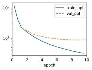
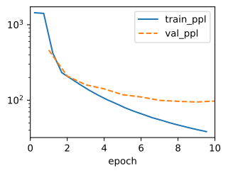
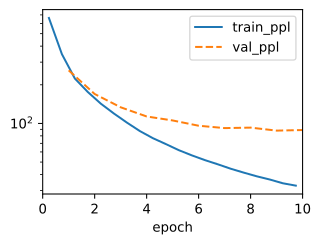
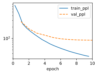
Since perplexity ranges over orders of magnitude during training, we plot it on a logarithmic axis. The curve starts near the vocabulary size, exactly the near-uniform initial model we constructed, and falls fast; at this aggressive learning rate the first few updates can transiently overshoot (clipping keeps the overshoot from becoming divergence, as an exercise invites you to verify). Let’s read off the final validation perplexity.
ppl_scratch = float(model.board.data['val_ppl'][-1].y)
print(f'validation perplexity {ppl_scratch:.1f}')
validation perplexity 98.3ppl_scratch = float(model.board.data['val_ppl'][-1].y)
print(f'validation perplexity {ppl_scratch:.1f}')validation perplexity 94.6total_loss = num_tokens = 0
for X_val, y_val in data.val_dataloader():
losses = model.loss(model(X_val), y_val, averaged=False)
total_loss += float(losses.sum())
num_tokens += losses.size
ppl_scratch = math.exp(total_loss / num_tokens)
print(f'validation perplexity {ppl_scratch:.1f}')validation perplexity 97.9ppl_scratch = float(model.board.data['val_ppl'][-1].y)
print(f'validation perplexity {ppl_scratch:.1f}')validation perplexity 91.2A perplexity in the tens-to-hundreds may look alarming next to the single-digit perplexities of the character-level models earlier in this chapter. Both numbers are correct, and the comparison is meaningless: our model chooses among 1,024 BPE tokens per step, a character model among 27 characters, and per-token perplexity cannot compare models with different tokenizers. This is precisely why Section 8.3 introduced bits per byte. Each of our tokens covers several bytes of text, so we convert: dividing the per-token surprisal \(\log_2(\textrm{ppl})\) by the average number of bytes per token gives the price in bits of each byte of validation text.
ids = d2l.numpy(data.X[data.num_train:data.num_train+data.num_val, 0]).tolist()
bytes_per_token = len(data.tokenizer.decode(ids).encode('utf-8')) / len(ids)
print(f'{bytes_per_token:.2f} bytes/token, '
f'{math.log2(ppl_scratch) / bytes_per_token:.2f} bits per byte')2.78 bytes/token, 2.38 bits per byte2.78 bytes/token, 2.36 bits per byte2.78 bytes/token, 2.38 bits per byte2.78 bytes/token, 2.34 bits per byteBack in Section 8.3, the character-tokenized trigram scored 2.68 bits per byte on this same text. Our BPE-level model, despite a per-token perplexity more than ten times larger, comes in below that, compressing the same text better. The lesson carries beyond this comparison: whenever two language models tokenize differently, compare bits per byte, never perplexity.
8.5.4 Generating Text
Once trained, the language model can do what Section 8.4 promised: continue a prefix. The predict method below first warms up on the user-supplied prefix, feeding its tokens one at a time to build up a hidden state without emitting anything. It then generates num_tokens new tokens, each time turning the current logits into a choice of next token and feeding that choice back in as the next input.
How should logits become a choice? The method offers the two simplest strategies. With temperature=0 it is greedy: always take the highest-scoring token. Otherwise it samples from the model’s next-token distribution after scaling the logits by \(1/T\) for temperature \(T\): values below 1 sharpen the distribution toward greedy behavior, values above 1 flatten it toward uniform randomness.
@d2l.add_to_class(RNNLMScratch)
@torch.no_grad()  # inference only: no autograd graph needed
def predict(self, prefix, num_tokens, tok, device=None, temperature=0.0,
            rng=None):
    outputs, state = tok.encode(prefix), None
    for i in range(len(outputs) - 1):  # Warm up on the prefix
        X = d2l.tensor([[outputs[i]]], device=device)
        _, state = self.rnn(self.embedding(X), state)
    rng = random.Random() if rng is None else rng
    for _ in range(num_tokens):  # Generate num_tokens continuation tokens
        X = d2l.tensor([[outputs[-1]]], device=device)
        rnn_outputs, state = self.rnn(self.embedding(X), state)
        logits = d2l.numpy(self.output_layer(rnn_outputs))[0, 0]
        if temperature == 0:
            outputs.append(int(logits.argmax()))
        else:
            weights = [math.exp(l) for l in
                       (logits - logits.max()) / temperature]
            outputs.append(rng.choices(range(len(weights)), weights)[0])
return tok.decode(outputs)@d2l.add_to_class(RNNLMScratch)
def predict(self, prefix, num_tokens, tok, device=None, temperature=0.0,
rng=None):
outputs, state = tok.encode(prefix), None
for i in range(len(outputs) - 1): # Warm up on the prefix
X = d2l.tensor([[outputs[i]]])
_, state = self.rnn(self.embedding(X), state)
rng = random.Random() if rng is None else rng
for _ in range(num_tokens): # Generate num_tokens continuation tokens
X = d2l.tensor([[outputs[-1]]])
rnn_outputs, state = self.rnn(self.embedding(X), state)
logits = d2l.numpy(self.output_layer(rnn_outputs))[0, 0]
if temperature == 0:
outputs.append(int(logits.argmax()))
else:
weights = [math.exp(l) for l in
(logits - logits.max()) / temperature]
outputs.append(rng.choices(range(len(weights)), weights)[0])
return tok.decode(outputs)@d2l.add_to_class(RNNLMScratch)
def predict(self, prefix, num_tokens, tok, device=None, temperature=0.0,
rng=None):
model = nnx.view(self, deterministic=True, use_running_average=True,
raise_if_not_found=False)
outputs, state = tok.encode(prefix), None
for i in range(len(outputs) - 1): # Warm up on the prefix
X = d2l.tensor([[outputs[i]]])
_, state = model.rnn(model.embedding(X), state)
rng = random.Random() if rng is None else rng
for _ in range(num_tokens): # Generate num_tokens continuation tokens
X = d2l.tensor([[outputs[-1]]])
rnn_outputs, state = model.rnn(model.embedding(X), state)
logits = d2l.numpy(model.output_layer(rnn_outputs))[0, 0]
if temperature == 0:
outputs.append(int(logits.argmax()))
else:
weights = [math.exp(l) for l in
(logits - logits.max()) / temperature]
outputs.append(rng.choices(range(len(weights)), weights)[0])
return tok.decode(outputs)@d2l.add_to_class(RNNLMScratch)
def predict(self, prefix, num_tokens, tok, device=None, temperature=0.0,
rng=None):
outputs, state = tok.encode(prefix), None
for i in range(len(outputs) - 1): # Warm up on the prefix
X = d2l.tensor([[outputs[i]]], ctx=device)
_, state = self.rnn(self.embedding(X), state)
rng = random.Random() if rng is None else rng
for _ in range(num_tokens): # Generate num_tokens continuation tokens
X = d2l.tensor([[outputs[-1]]], ctx=device)
rnn_outputs, state = self.rnn(self.embedding(X), state)
logits = d2l.numpy(self.output_layer(rnn_outputs))[0, 0]
if temperature == 0:
outputs.append(int(logits.argmax()))
else:
weights = [math.exp(l) for l in
(logits - logits.max()) / temperature]
outputs.append(rng.choices(range(len(weights)), weights)[0])
return tok.decode(outputs)Greedy decoding first. Note that the prefix is real text, not token ids: the tokenizer trained by the pipeline (data.tokenizer) encodes it on the way in and decodes the generated ids on the way out.
d2l.print_wrapped(repr(model.predict('the time traveller', 50,
                                     data.tokenizer, d2l.try_gpu())))
'the time traveller. I had the same. I was not beenred, and the same. I was
not beenred, and the same. I was not beenred, and the same. I was not
beenred, and the same. I was not been'd2l.print_wrapped(repr(model.predict('the time traveller', 50,
data.tokenizer)))"the time traveller. I had not a line of the Time Traveller. 'I'm\nthe
simple the Time Traveller. I had not a line of the Time Traveller.
'I'm\nthe simple the Time Traveller. I"d2l.print_wrapped(repr(model.predict('the time traveller', 50,
data.tokenizer)))"the time traveller had\ndeerved in\ntheset of the\nside of\nthem.\n\n'Ined
the Time Traveller.\n\n'Ined the Time Traveller.\n\n'Ined the Time
Traveller"d2l.print_wrapped(repr(model.predict('the time traveller', 50,
data.tokenizer, d2l.try_gpu())))'the time traveller, I saw the\nside\nfeet, I\nface, I saw the\nside\nfeet,
I\nface, I saw the\nside\nfeet, I\nface, I'The continuation is locally plausible Wells, but it does not stay interesting for long. Greedy decoding is deterministic, and it tends to fall into repetition: once the hidden state drifts into a high-probability neighborhood, the same phrases recur again and again. Sampling with temperature breaks such loops at the price of occasional strange choices, and lowering the temperature interpolates back toward the greedy behavior.
for T in (1.0, 0.5):
    d2l.print_wrapped(model.predict('the time traveller', 30, data.tokenizer,
                                    d2l.try_gpu(), temperature=T,
                                    rng=random.Random(0)))
the time travellerions move it was sensle of the Lil of an with the L Space
this curesivity of the little peoplepeove
the time traveller of the Time Traveller. 'I wonderful of the great
diffto the Morlocks, and I could see the panelightfor T in (1.0, 0.5):
d2l.print_wrapped(model.predict('the time traveller', 30, data.tokenizer,
temperature=T, rng=random.Random(0)))the time travellerred phating of the increes of impachin. Filbyare got
tooild of my imagine, in itressves
the time travellers. The
man. I had nothing of the bronze of the daylight, and then I had
delsidefor T in (1.0, 0.5):
d2l.print_wrapped(model.predict('the time traveller', 30, data.tokenizer,
temperature=T, rng=random.Random(0)))the time travellerom his sanil to disacal meerely I must have a sudden
muchions of fant Machineveral
well useping
the time traveller had
dorsson which
these form of the
first on of the
telling of
these wastefor T in (1.0, 0.5):
d2l.print_wrapped(model.predict('the time traveller', 30, data.tokenizer,
d2l.try_gpu(), temperature=T,
rng=random.Random(0)))the time travellerook vightdle. It was anse acley this leed even might like
workelftagge
wellso sat
the time traveller, I had
wellt the
sideer, I saw a vivident in the
surmit. At firstNeither knob fixes the underlying problem: repetition, incoherence, and the trade-off between them are properties of how we choose tokens, not just of the model. Choosing well is a rich topic with a modern toolkit of its own, and Section 8.7 is devoted to it. For now we have what we need: a trained model and a way to watch it write.
8.5.5 Concise Implementation
Implementing the RNN from scratch was instructive, but frameworks ship recurrent layers that bundle the cell and the time loop into one optimized call. The RNN class below wraps the framework layer while keeping exactly the interface of RNNScratch: it consumes a (num_steps, batch_size, num_inputs) tensor and an optional state, and returns per-step hidden states plus the final state.
Flax NNX provides SimpleCell for a vanilla recurrent cell. Unlike a layer that processes an entire sequence at once, the cell consumes one time step and an explicit hidden state; nnx.RNN scans it over the input sequence.
class RNN(d2l.Module):
    """The RNN model implemented with high-level APIs."""
    def __init__(self, num_inputs, num_hiddens):
        super().__init__()
        self.save_hyperparameters()
        self.rnn = nn.RNN(num_inputs, num_hiddens)

    def forward(self, inputs, H=None):
        return self.rnn(inputs, H)
class RNN(d2l.Module):
"""The RNN model implemented with high-level APIs."""
def __init__(self, num_inputs, num_hiddens):
super().__init__()
self.save_hyperparameters()
self.rnn = tf.keras.layers.SimpleRNN(
num_hiddens, return_sequences=True, return_state=True)
def forward(self, inputs, H=None):
# The keras layer is batch-major: transpose in and out
outputs, H = self.rnn(tf.transpose(inputs, perm=[1, 0, 2]), H)
return tf.transpose(outputs, perm=[1, 0, 2]), Hclass RNN(nnx.Module):
"""The RNN model implemented with high-level APIs."""
def __init__(self, num_inputs, num_hiddens, rngs=None):
rngs = nnx.Rngs(0) if rngs is None else rngs
self.num_inputs, self.num_hiddens = num_inputs, num_hiddens
self.rnn = nnx.RNN(
nnx.SimpleCell(num_inputs, num_hiddens, rngs=rngs),
time_major=True, return_carry=True, rngs=rngs)
def __call__(self, inputs, H=None):
H, outputs = self.rnn(inputs, initial_carry=H)
return outputs, Hclass RNN(d2l.Module):
"""The RNN model implemented with high-level APIs."""
def __init__(self, num_inputs, num_hiddens):
super().__init__()
self.save_hyperparameters()
self.rnn = gluon.rnn.RNN(num_hiddens)
def forward(self, inputs, H=None):
if H is None:
H, = self.rnn.begin_state(inputs.shape[1], ctx=inputs.ctx)
outputs, (H, ) = self.rnn(inputs, (H, ))
return outputs, HBecause the interface is unchanged, the language model wrapper carries over by inheritance: RNNLM subclasses RNNLMScratch and merely swaps the hand-rolled embedding table and output projection for the framework’s embedding and dense layers. Training, evaluation, and predict are all inherited. One detail deserves attention: several frameworks initialize embedding tables at the small scale appropriate for dense-layer weights, which starves the recurrence of input signal on this task, so where needed we request the unit-normal initialization that embeddings conventionally use (and that our scratch model, and PyTorch’s nn.Embedding, already default to).
class RNNLM(d2l.RNNLMScratch):
    """The RNN-based language model implemented with high-level APIs."""
    def init_params(self):
        self.emb = nn.Embedding(self.vocab_size, self.rnn.num_inputs)
        self.linear = nn.LazyLinear(self.vocab_size)

    def embedding(self, X):
        return self.emb(X.T)

    def output_layer(self, hiddens):
        return d2l.swapaxes(self.linear(hiddens), 0, 1)
class RNNLM(d2l.RNNLMScratch):
"""The RNN-based language model implemented with high-level APIs."""
def init_params(self):
self.emb = tf.keras.layers.Embedding(
self.vocab_size, self.rnn.num_inputs,
embeddings_initializer=tf.keras.initializers.RandomNormal(
stddev=1))
self.linear = tf.keras.layers.Dense(self.vocab_size)
def embedding(self, X):
return self.emb(tf.transpose(X))
def output_layer(self, hiddens):
return d2l.transpose(self.linear(hiddens), (1, 0, 2))class RNNLM(d2l.RNNLMScratch):
"""The RNN-based language model implemented with high-level APIs."""
def __init__(self, rnn, vocab_size, lr=0.01, rngs=None):
d2l.Classifier.__init__(self)
self.save_hyperparameters(ignore=['rnn', 'rngs'])
self.rnn = rnn
rngs = nnx.Rngs(2) if rngs is None else rngs
self.emb = nnx.Embed(vocab_size, rnn.num_inputs,
embedding_init=nnx.initializers.normal(1.0),
rngs=rngs)
self.linear = nnx.Linear(rnn.num_hiddens, vocab_size, rngs=rngs)
def embedding(self, X):
return self.emb(X.T)
def output_layer(self, hiddens):
return d2l.swapaxes(self.linear(hiddens), 0, 1)class RNNLM(d2l.RNNLMScratch):
"""The RNN-based language model implemented with high-level APIs."""
def init_params(self):
self.emb = nn.Embedding(self.vocab_size, self.rnn.num_inputs,
weight_initializer=init.Normal(1))
self.linear = nn.Dense(self.vocab_size, flatten=False)
self.initialize()
def embedding(self, X):
return self.emb(X.T)
def output_layer(self, hiddens):
return d2l.swapaxes(self.linear(hiddens), 0, 1)Before training, let’s make a prediction with the randomly initialized model. Since the network has learned nothing, the continuation is byte soup; the replacement characters appear where generated ids decode to bytes that do not form valid UTF-8. It is still a useful check that the wiring, from tokenizer through model and back, is sound.
rnn = RNN(num_inputs=64, num_hiddens=128)
model = RNNLM(rnn, vocab_size=len(data.vocab), lr=4)
with d2l.try_gpu():
rnn = RNN(num_inputs=64, num_hiddens=128)
model = RNNLM(rnn, vocab_size=len(data.vocab), lr=4)
rnn = RNN(num_inputs=64, num_hiddens=128)
model = RNNLM(rnn, vocab_size=len(data.vocab), lr=4)rnn = RNN(num_inputs=64, num_hiddens=128)
model = RNNLM(rnn, vocab_size=len(data.vocab), lr=4)model.predict('it has', 20, data.tokenizer)'it has>oratoryV part eyes� blackhed le mind�pp downultJ Man black seemed were8''it has kind could� comeher� d\x0eill might two�ence cle diff awaylfDileead''it has m\x1d e5asause sornessare ex( lab� Thenhing�imes now strange''it has\x1aning diffreat o wentous anotherreatreat o wentous anotherreatreat o wentous another'Training is the same call as before, with the same hyperparameters.
trainer = d2l.Trainer(max_epochs=10, gradient_clip_val=1, num_gpus=1)
model.board.yscale = 'log'
t0 = time.time()
trainer.fit(model, data)
t_concise = time.time() - t0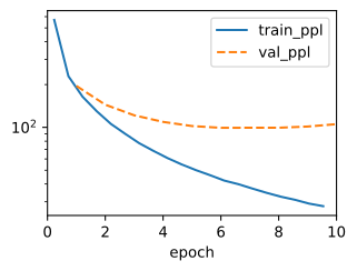
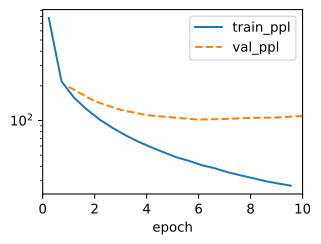
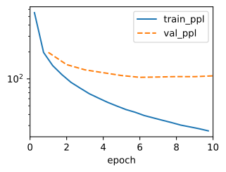
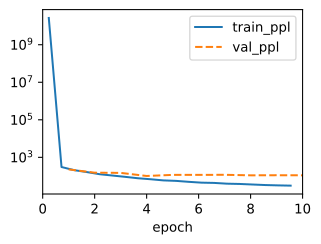
The trained model reaches a validation perplexity in the same range as the from-scratch implementation, somewhat higher in some frameworks, and its samples read the same.
ppl_concise = float(model.board.data['val_ppl'][-1].y)
pred = model.predict('the time traveller', 30, data.tokenizer, d2l.try_gpu())
d2l.print_wrapped(f'perplexity {ppl_concise:.1f}, {pred!r}')
perplexity 101.1, "the time traveller.\nThe Time Traveller'ser--
aitsie.\n\n'Incendly, and\nwere was a f"ppl_concise = float(model.board.data['val_ppl'][-1].y)
pred = model.predict('the time traveller', 30, data.tokenizer)
d2l.print_wrapped(f'perplexity {ppl_concise:.1f}, {pred!r}')perplexity 104.1, "the time traveller had\nafter heard the\nface,
and\ntoolailed to\nmonze.\n\n'I was"total_loss = num_tokens = 0
for X_val, y_val in data.val_dataloader():
losses = model.loss(model(X_val), y_val, averaged=False)
total_loss += float(losses.sum())
num_tokens += losses.size
ppl_concise = math.exp(total_loss / num_tokens)
pred = model.predict('the time traveller', 30, data.tokenizer)
d2l.print_wrapped(f'perplexity {ppl_concise:.1f}, {pred!r}')perplexity 109.1, 'the time traveller of the Time Traveller, and, I had not
been\nfast or four\nshelposs\ntime. I could'ppl_concise = float(model.board.data['val_ppl'][-1].y)
pred = model.predict('the time traveller', 30, data.tokenizer, d2l.try_gpu())
d2l.print_wrapped(f'perplexity {ppl_concise:.1f}, {pred!r}')perplexity 132.4, "the time travellerzy.\nThe Time Traveller's face.\n\n'I
was a lineervitution.\n\n'I was a"8.5.5.1 Scratch versus Concise, Measured
Since we timed both training runs, we can put the comparison in a small table rather than assert it.
print(f'{"model":>8} {"time (s)":>9} {"val ppl":>8}')
for name, t, p in [('scratch', t_scratch, ppl_scratch),
                   ('concise', t_concise, ppl_concise)]:
print(f'{name:>8} {t:>9.1f} {p:>8.1f}') model time (s) val ppl
scratch 16.9 98.3
concise 6.5 101.1 model time (s) val ppl
scratch 56.0 94.6
concise 41.6 104.1 model time (s) val ppl
scratch 18.5 97.9
concise 14.2 109.1 model time (s) val ppl
scratch 88.6 91.2
concise 32.3 132.4The framework layer wins by a wide margin. The reason is kernel fusion: our scratch loop launches several small GPU operations per time step from Python, and at this model size the per-launch overhead dwarfs the arithmetic, while nn.RNN executes the whole unrolled recurrence inside one fused library kernel.
The margin here is smaller than in the PyTorch tab, and it moves around from run to run. The reason is that Keras provides no fused GPU kernel for the vanilla SimpleRNN (only its LSTM and GRU layers have one), so both versions execute as tf.function-compiled graphs of per-step operations, and neither enjoys a fused advantage. Fused kernels win when they exist; the LSTM and GRU layers of Chapter 12 show the speedup this layer is missing.
The gap is modest here because both versions are JIT-compiled end to end: our scratch loop is unrolled and fused by XLA just like the library cell, and the remaining difference is mostly compilation and dispatch overhead. The comparison is starker in eager frameworks, where the scratch loop pays a Python-level launch cost at every time step.
The framework layer wins by a comfortable margin. The reason is kernel fusion: our scratch loop launches several small GPU operations per time step from Python, and at this model size the per-launch overhead dwarfs the arithmetic, while rnn.RNN executes the whole unrolled recurrence inside one fused library kernel.
At this model size the absolute difference is seconds. At the scale of Chapter 12’s gated cells, with more parameters per step, deeper stacks, and longer sequences, the same per-step overhead multiplies, and the fused layer becomes the only sensible choice. We will keep the scratch idiom for exposition and the framework layer for every model we actually train at length.
8.5.6 Summary
We implemented an RNN language model twice. The from-scratch version makes the anatomy explicit: an embedding lookup replaces the wasteful one-hot encoding (it is the same linear map, with trainable rows), a recurrent cell carries a fixed-size state across time steps, and a shared output layer produces next-token logits at every step. Training with gradient clipping bounds the damage any one exploding gradient can do, though it does nothing for vanishing gradients. Because each minibatch window starts from a fresh state, backpropagation is truncated at the window length, a compromise that Section 8.6 examines. Perplexities measured over different vocabularies are incomparable, so we converted to bits per byte to see that our BPE-level model genuinely improves on a character-level one. Finally, the trained model generates text: greedy decoding is fluent but circles, temperature sampling trades repetition for noise, and doing better is the subject of Section 8.7. The concise implementation collapses all of this into framework layers with the same interface and, where fused kernels exist, meaningfully better speed.
8.5.7 Exercises
- [code] Gradient clipping ablation.
d2l.Trainerapplies the projection Equation 8.5.2 whenevergradient_clip_valis positive.- Train
RNNLMScratchwithgradient_clip_val=0atlr=4. Then halve the learning rate until the unclipped run no longer diverges. How does the validation perplexity of that run after ten epochs compare with that of the clipped run atlr=4? - Replace \(\tanh\) by ReLU in
RNNScratchand train again, with and without clipping. Is clipping still needed? Explain the difference from the \(\tanh\) cell in terms of the range of the hidden state.
- Train
- [code] Usable history. Every training window starts from a zero state, so the model is never trained to use more than
num_stepstokens of context.predict, by contrast, carries the state across the whole prefix and every generated token. Evaluate the trained model on 512 consecutive validation tokens in two ways: resetting the state to zero every 32 tokens as in training, and carrying the state across all 512 tokens. Compare the average cross-entropy of the two. Does the carried state help, hurt, or make no difference, and what does the answer say about the states the model reaches beyond its training horizon? - [code] Hyperparameters and data budget.
- Adjust the number of epochs, hidden units, embedding dimension,
num_steps, and learning rate to lower the validation perplexity. What is the lowest value you reach? How does the relative improvement in bits per byte compare with the relative improvement in perplexity, and why? - Restore the pipeline default
num_train=10000and train for 100 epochs. Compare the training and validation perplexity curves and explain what you see. Consecutive windows overlap by 31 tokens, so how many parameters does the model have per distinct training token in this regime?
- Adjust the number of epochs, hidden units, embedding dimension,
- [code] Vocabulary size and bits per byte. ● Rebuild the dataset with
vocab_sizeset to 512, 1,024, 2,048, and 4,096 ind2l.TimeMachineand retrain with the same architecture and training procedure. The number of windowslen(data.X)depends on the vocabulary size, so replace the fixed split of 50,000 training and 5,000 validation windows by a fractional one. After building each dataset, setdata.num_traintoint(0.8 * len(data.X))anddata.num_valtolen(data.X) - data.num_train. Every model then trains and validates on about the same stretch of text. The per-token perplexities of these models are not comparable, so compare them by bits per byte.- Which vocabulary size gives the lowest bits per byte?
- How do the parameter counts of the embedding table and the output layer, and the length of the corpus in tokens, change with the vocabulary size? Which of these effects best explains the trend you measured?
- Weight tying savings. Weight tying sets the embedding dimension equal to the number of hidden units and uses \(\mathbf{W}_\textrm{e}^\top\) as the output projection in place of \(\mathbf{W}_{\textrm{hq}}\) (Press and Wolf 2017; Inan et al. 2017). How many parameters does tying save at \(|\mathcal{V}| = 1{,}024\) with 128 hidden units? GPT-2 small ties its \(50{,}257 \times 768\) token embedding to its output layer. How many parameters would untying add there, and what fraction of the model’s roughly 124 million parameters is that?
- [code] Weight tying. ● Set the embedding dimension equal to the number of hidden units, 128, and use \(\mathbf{W}_\textrm{e}^\top\) as the output projection in place of \(\mathbf{W}_{\textrm{hq}}\) in
RNNLMScratch.RNNLMScratchinitializes \(\mathbf{W}_\textrm{e}\) at unit scale and \(\mathbf{W}_{\textrm{hq}}\) at scalesigma. What happens to the initial perplexity once the two are tied, and how do you restore a near-uniform initial prediction?- Train the tied model and an untied model with a 128-dimensional embedding and 128 hidden units, and compare their validation perplexities.
- [code] Cross-book generalization. ● Subclass
d2l.TimeMachineand override_downloadto return the text of a different H. G. Wells novel, such as The War of the Worlds (Project Gutenberg ebook 36). Train the tokenizer and the model on it.- Evaluate the model on held-out text of its own novel and on The Time Machine, encoding both with the new novel’s tokenizer. Report perplexity and bits per byte for both.
- Write \(s = \log_2(\textrm{ppl})\) for the per-token surprisal and \(b\) for the bytes per token of an evaluated text, so that bits per byte is \(s / b\). The ratio of bits per byte on The Time Machine (TM) to bits per byte on the held-out text of the new novel (own) factors as \[\frac{s_\textrm{TM}}{s_\textrm{own}} \cdot \frac{b_\textrm{own}}{b_\textrm{TM}}.\] The first factor reflects the model’s predictions and the second the tokenizer’s compression. Measure both factors. Which lies further from one?
- [code] Scratch versus concise timing.
t_scratchandt_concisetime ten epochs ofRNNLMScratchandRNNLMwith 128 hidden units, 32-token windows, and a batch size of 1,024.- Vary
num_hiddensover 32, 128, and 512 andnum_stepsover 16, 32, and 128, and tabulate the ratiot_scratch / t_concisefor each setting. In which direction does the ratio move with each hyperparameter? - Repeat the default setting with a batch size of 64. Explain the changes you measure: which of per-step launch overhead, arithmetic per step, and compilation dominates in each regime?
- Vary