import os

os.makedirs(os.path.join('..', 'data'), exist_ok=True)
data_file = os.path.join('..', 'data', 'house_tiny.csv')
with open(data_file, 'w') as f:
    f.write('''NumRooms,RoofType,Area,Price
3,Slate,1500,210000
,Tile,2100,290000
2,,850,127500
4,Slate,1940,258000
,,1200,168000
3,Tile,1650,225000
5,Slate,2600,375000
2,,900,142000
,Tile,1750,240000
4,,2050,295000''')1.2 Data Preprocessing
So far, our synthetic data has arrived as ready-made tensors. Real tabular datasets usually require several preprocessing decisions: how to represent missing values, how to encode categories, and whether to rescale numerical features. These decisions determine what information the model receives.
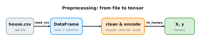
The pandas library (McKinney 2010) provides convenient tools for loading, inspecting, cleaning, and encoding tabular data. This section applies those tools to a small dataset and then converts the result to tensors. For a broader treatment, see the official tutorial. Figure 1.2.1 previews the steps in this section.
1.2.1 Load and Inspect
1.2.1.1 Reading the Dataset
Comma-separated values (CSV) files are ubiquitous for storing tabular (spreadsheet-like) data. Each line is one record of several comma-separated fields, e.g., “Albert Einstein,March 14 1879,Ulm,Federal polytechnic school”. To demonstrate, we write a small dataset of homes to ../data/house_tiny.csv. Each row is a home; the columns are the number of rooms (NumRooms), the roof type (RoofType), the floor area in square feet (Area), and the sale price (Price). An empty field denotes a missing entry.
Now we import pandas and load the dataset with read_csv.
import pandas as pd

data = pd.read_csv(data_file)
data
NumRooms RoofType Area Price
0 3.0 Slate 1500 210000
1 NaN Tile 2100 290000
2 2.0 NaN 850 127500
3 4.0 Slate 1940 258000
4 NaN NaN 1200 168000
5 3.0 Tile 1650 225000
6 5.0 Slate 2600 375000
7 2.0 NaN 900 142000
8 NaN Tile 1750 240000
9 4.0 NaN 2050 295000pandas has replaced the empty fields with a special NaN (not a number) marker. These are missing values, and dealing with them is one of the central chores of data preprocessing.
1.2.1.2 Knowing Your Data
Inspect the data before transforming it. The shape tells you how much data you have; the dtypes tell you how pandas interpreted each column: numeric (int64/float64) versus non-numeric strings (str/object, i.e. categorical or text); and describe summarizes the numeric columns, surfacing ranges and obvious outliers at a glance.
data.dtypesNumRooms float64
RoofType str
Area int64
Price int64
dtype: objectNumRooms came in as float64 (not int) precisely because it contains a NaN; RoofType is a string column, our cue that it is categorical and will need encoding. The numeric summary:
data.describe() NumRooms Area Price
count 7.000000 10.000000 10.000000
mean 3.285714 1654.000000 233050.000000
std 1.112697 556.421104 76128.710455
min 2.000000 850.000000 127500.000000
25% 2.500000 1275.000000 178500.000000
50% 3.000000 1700.000000 232500.000000
75% 4.000000 2022.500000 282000.000000
max 5.000000 2600.000000 375000.000000The three numeric columns live on very different scales: rooms in the single digits, area in the thousands, price in the hundred-thousands. Keep that in mind; it returns below.
1.2.1.3 Separating Inputs and Targets
In supervised learning we predict a target from a set of inputs. The first step is to split the columns accordingly so that we only ever preprocess the inputs, never peeking at or transforming the target as if it were a feature. Here the last column, Price, is the target; the rest are inputs. We select by integer position with iloc (selecting by column name works too, and is often clearer):
inputs, targets = data.iloc[:, :3], data.iloc[:, 3]
inputs
NumRooms RoofType Area
0 3.0 Slate 1500
1 NaN Tile 2100
2 2.0 NaN 850
3 4.0 Slate 1940
4 NaN NaN 1200
5 3.0 Tile 1650
6 5.0 Slate 2600
7 2.0 NaN 900
8 NaN Tile 1750
9 4.0 NaN 20501.2.2 Clean and Encode
1.2.2.1 Handling Missing Values
Missing values are unavoidable in real datasets, and how we handle them can change what a model learns. First, measure the problem: how many values are missing, and where?
inputs.isna().sum()NumRooms 3
RoofType 4
Area 0
dtype: int64There are three broad ways to respond, each with a cost:
- Deletion: drop rows (or columns) that contain a
NaN. Simple, but it throws data away and can bias the result if values are not missing at random. - Imputation: fill each
NaNwith an estimate (a column statistic, or a model’s prediction). Keeps every row, but injects assumptions and shrinks the data’s variance. - Indicator: add a boolean “was-missing” column so the model can learn from the fact that a value was absent.
Deletion is tempting but expensive on small data. Dropping every row with any missing entry here leaves only a fraction of the dataset:
len(inputs.dropna()), len(inputs)(4, 10)Only four of ten rows remain, so we impute instead. For a numerical column the simplest estimate is the column mean (use the median when the column is skewed). fillna applies it. We impute the numerical columns now and leave the categorical RoofType for the next section, where treating “missing” as its own category is the natural fix.
inputs = inputs.fillna(inputs.mean(numeric_only=True))
inputs
NumRooms RoofType Area
0 3.000000 Slate 1500
1 3.285714 Tile 2100
2 2.000000 NaN 850
3 4.000000 Slate 1940
4 3.285714 NaN 1200
5 3.000000 Tile 1650
6 5.000000 Slate 2600
7 2.000000 NaN 900
8 3.285714 Tile 1750
9 4.000000 NaN 2050NumRooms and Area are now filled with their column means; RoofType’s missing entries remain, to be handled by encoding.
1.2.2.2 Encoding Categorical Features
Models consume numbers, so the RoofType strings must be encoded. The standard choice for a nominal category (one with no inherent order) is one-hot encoding: one new 0/1 column per category. We avoid mapping categories to integers like Slate=0, Tile=1, because that invents a false ordering and magnitude the model would wrongly exploit. pd.get_dummies does the conversion; dummy_na=True adds a column for the missing category, which is exactly the indicator strategy from the previous section, applied to a categorical column:
inputs = pd.get_dummies(inputs, dummy_na=True, dtype=float)
inputs
NumRooms Area RoofType_Slate RoofType_Tile RoofType_nan
0 3.000000 1500 1.0 0.0 0.0
1 3.285714 2100 0.0 1.0 0.0
2 2.000000 850 0.0 0.0 1.0
3 4.000000 1940 1.0 0.0 0.0
4 3.285714 1200 0.0 0.0 1.0
5 3.000000 1650 0.0 1.0 0.0
6 5.000000 2600 1.0 0.0 0.0
7 2.000000 900 0.0 0.0 1.0
8 3.285714 1750 0.0 1.0 0.0
9 4.000000 2050 0.0 0.0 1.0RoofType has become three columns (RoofType_Slate, RoofType_Tile, and RoofType_nan); the already-imputed numerical columns pass through untouched. Every column is now numeric.
One caveat: one-hot encoding a high-cardinality column (thousands of distinct values, such as ZIP codes) explodes the feature count and is rarely useful. Such columns call for embeddings, which we meet in Section 18.5.
1.2.3 Scale and Convert
1.2.3.1 Numerical Features
Every entry is now numeric and complete. As promised when describe first surfaced it, though, the continuous columns still span very different scales (NumRooms ≈ 3, Area ≈ 1700). Left as-is, the large-magnitude feature dominates distances and gradients, making optimization ill-conditioned: gradient descent zig-zags along the large-scale direction instead of heading straight for the minimum (Section 26.5 treats conditioning in depth). The standard fix is standardization: subtract the mean and divide by the standard deviation, so each continuous feature has roughly zero mean and unit variance. (We leave the one-hot columns alone; they are already 0/1.)
continuous = ['NumRooms', 'Area']
inputs[continuous] = (inputs[continuous] - inputs[continuous].mean()) \
                     / inputs[continuous].std()
inputs
NumRooms Area RoofType_Slate RoofType_Tile RoofType_nan
0 -0.314485 -0.276769 1.0 0.0 0.0
1 0.000000 0.801551 0.0 1.0 0.0
2 -1.415185 -1.444949 0.0 0.0 1.0
3 0.786214 0.513999 1.0 0.0 0.0
4 0.000000 -0.815929 0.0 0.0 1.0
5 -0.314485 -0.007189 0.0 1.0 0.0
6 1.886913 1.700151 1.0 0.0 0.0
7 -1.415185 -1.355089 0.0 0.0 1.0
8 0.000000 0.172531 0.0 1.0 0.0
9 0.786214 0.711691 0.0 0.0 1.0A subtlety to flag now and revisit later: the statistics used to impute (the column means earlier) and to standardize (mean and standard deviation) must be computed on the training data only, then reused for validation and test data. Computing them over the whole dataset leaks information about the test set into training and inflates your reported performance. We return to training/validation/test splits in Section 2.6 and practice leak-free preprocessing on a real dataset in Section 4.7.
1.2.3.2 Conversion to Tensor Format
Now that inputs and targets are entirely numeric, we can load them into tensors (recall Section 1.1). Pandas hands off to NumPy via to_numpy, and the tensor constructor wraps that array. Deep learning typically uses 32-bit floats; to_numpy(dtype=float) gives 64-bit, so in real pipelines you would cast down to float32 to save memory and match the framework defaults.
import torch

X = torch.tensor(inputs.to_numpy(dtype=float))
y = torch.tensor(targets.to_numpy(dtype=float))
X, y
(tensor([[-0.3145, -0.2768, 1.0000, 0.0000, 0.0000],
[ 0.0000, 0.8016, 0.0000, 1.0000, 0.0000],
[-1.4152, -1.4449, 0.0000, 0.0000, 1.0000],
[ 0.7862, 0.5140, 1.0000, 0.0000, 0.0000],
[ 0.0000, -0.8159, 0.0000, 0.0000, 1.0000],
[-0.3145, -0.0072, 0.0000, 1.0000, 0.0000],
[ 1.8869, 1.7002, 1.0000, 0.0000, 0.0000],
[-1.4152, -1.3551, 0.0000, 0.0000, 1.0000],
[ 0.0000, 0.1725, 0.0000, 1.0000, 0.0000],
[ 0.7862, 0.7117, 0.0000, 0.0000, 1.0000]], dtype=torch.float64),
tensor([210000., 290000., 127500., 258000., 168000., 225000., 375000., 142000.,
240000., 295000.], dtype=torch.float64))import tensorflow as tf
X = tf.constant(inputs.to_numpy(dtype=float))
y = tf.constant(targets.to_numpy(dtype=float))
X, y(<tf.Tensor: shape=(10, 5), dtype=float64, numpy=
array([[-0.31448545, -0.2767688 , 1. , 0. , 0. ],
[ 0. , 0.80155119, 0. , 1. , 0. ],
[-1.41518453, -1.44494879, 0. , 0. , 1. ],
[ 0.78621363, 0.5139992 , 1. , 0. , 0. ],
[ 0. , -0.81592879, 0. , 0. , 1. ],
[-0.31448545, -0.0071888 , 0. , 1. , 0. ],
[ 1.88691271, 1.70015119, 1. , 0. , 0. ],
[-1.41518453, -1.35508879, 0. , 0. , 1. ],
[ 0. , 0.1725312 , 0. , 1. , 0. ],
[ 0.78621363, 0.71169119, 0. , 0. , 1. ]])>,
<tf.Tensor: shape=(10,), dtype=float64, numpy=
array([210000., 290000., 127500., 258000., 168000., 225000., 375000.,
142000., 240000., 295000.])>)from jax import numpy as jnp
X = jnp.array(inputs.to_numpy(dtype=float))
y = jnp.array(targets.to_numpy(dtype=float))
X, y(Array([[-0.31448546, -0.2767688 , 1. , 0. , 0. ],
[ 0. , 0.8015512 , 0. , 1. , 0. ],
[-1.4151845 , -1.4449488 , 0. , 0. , 1. ],
[ 0.78621364, 0.5139992 , 1. , 0. , 0. ],
[ 0. , -0.8159288 , 0. , 0. , 1. ],
[-0.31448546, -0.0071888 , 0. , 1. , 0. ],
[ 1.8869127 , 1.7001512 , 1. , 0. , 0. ],
[-1.4151845 , -1.3550888 , 0. , 0. , 1. ],
[ 0. , 0.1725312 , 0. , 1. , 0. ],
[ 0.78621364, 0.7116912 , 0. , 0. , 1. ]], dtype=float32),
Array([210000., 290000., 127500., 258000., 168000., 225000., 375000.,
142000., 240000., 295000.], dtype=float32))from mxnet import np
X = np.array(inputs.to_numpy(dtype=float))
y = np.array(targets.to_numpy(dtype=float))
X, y(array([[-0.31448546, -0.2767688 , 1. , 0. , 0. ],
[ 0. , 0.8015512 , 0. , 1. , 0. ],
[-1.4151845 , -1.4449488 , 0. , 0. , 1. ],
[ 0.78621364, 0.5139992 , 1. , 0. , 0. ],
[ 0. , -0.8159288 , 0. , 0. , 1. ],
[-0.31448546, -0.0071888 , 0. , 1. , 0. ],
[ 1.8869127 , 1.7001512 , 1. , 0. , 0. ],
[-1.4151845 , -1.3550888 , 0. , 0. , 1. ],
[ 0. , 0.1725312 , 0. , 1. , 0. ],
[ 0.78621364, 0.7116912 , 0. , 0. , 1. ]]),
array([210000., 290000., 127500., 258000., 168000., 225000., 375000.,
142000., 240000., 295000.]))Subsequent sections use these tensors for model computation and differentiation.
1.2.4 Discussion
The main preprocessing steps are to inspect the data, separate inputs from targets, handle missing values, encode categorical variables, scale numerical variables when appropriate, and convert the result to tensors. A larger example appears in Section 4.7.
Rather than a single CSV, a dataset may be spread across many files pulled from a relational database (customer addresses in one table, purchases in another) that must be joined first. Beyond categorical and numeric fields, practitioners face text, images, audio, and point clouds, each needing its own pipeline (we meet these in the computer vision and natural language processing chapters). For data that does not fit in memory, pandas is the wrong tool; columnar formats like Parquet and out-of-core engines take over. And throughout, watch data quality: outliers and recording errors must be caught before training, and plotting a column with a library such as matplotlib is often the fastest way to spot them. For the transforms in this section (imputation, encoding, scaling) and for chaining them into reproducible pipelines, see sklearn.impute and sklearn.preprocessing.
1.2.5 Exercises
[code] Inspecting a real dataset. Load a dataset from the UCI Machine Learning Repository, for example Abalone, and inspect it with
dtypes,describe, andisna. Report what fraction of the values are missing and what fraction of the columns are numerical, categorical, or text, and state which of the preprocessing steps of this section the dataset actually needs.[code] Indexing by name. This section splits
databy position withdata.iloc[:, :3]anddata.iloc[:, 3]. Suppose a new version ofhouse_tiny.csvadds a columnYearBuiltbetweenAreaandPrice.- State what the positional split then puts into
inputsandtargets, and whether any later line of the section’s code raises an error. - Rewrite the split with column names so that
targetsholdsPriceandinputsholds every other column, for the new file and for the original one. The pandas user guide on indexing lists the options.
- State what the positional split then puts into
[code] Imputation strategies. Fill the missing values in
NumRoomsin three ways: with the column mean, with the column median, and with the column mean plus a “was-missing” indicator column.- For the mean fill and the median fill, compute the mean and the standard deviation of the filled column, compare them with those of the observed values, and explain the direction of each change.
- Suppose that in a larger dataset
NumRoomsis missing mostly for large homes. State what a model sees for those homes after mean imputation alone. Then explain how a model that predicts the price as a weighted sum of its features plus a constant can use the indicator column to correct its predictions for them. - State what each of the three treatments assumes about why the values are missing.
Adapted from Kaggle Learn, Intermediate Machine Learning, Exercise 2.
[code] Where leakage hides. This section fills the missing
NumRoomsentries with the mean of all observed values and standardizesNumRoomsandAreawith the mean and standard deviation of all ten rows. Treat the first eight rows ofdataas training data and the last two as test data.- Redo the imputation and the standardization with statistics computed on the training rows only and applied unchanged to the test rows. Compare the standardized test rows with those of the whole-dataset recipe.
- Explain what the whole-dataset recipe lets the model learn about the test rows that the training-only recipe does not.
- Suppose a feature is constant on the training rows but not on the test rows. State what the training-only recipe produces for that feature on each split, and propose a fix.
[code] Memory per row. Use
data.memory_usage(deep=True)to find how many bytes per row theRoofTypecolumn and theAreacolumn ofdataoccupy in memory. Compare each with the average number of bytes the same field takes inhouse_tiny.csv.[code] Scaling limits. ● Estimate how many rows of a table with the columns of
house_tiny.csvyou can load withpd.read_csvon your machine. Write synthetic CSV files with the four columns ofhouse_tiny.csvand \(10^5\), \(10^6\), and \(10^7\) random rows. For each file, timepd.read_csvand record the memory of the resulting DataFrame. Extrapolate both measurements linearly. Find the number of rows at which the DataFrame would fill your machine’s memory and the number at which loading would take ten minutes, and state which limit comes first.High-cardinality categories. One-hot encoding turns a categorical column with \(k\) distinct values into \(k\) columns, plus one more with
dummy_na=True.- A table of \(n = 10^6\) homes has a
ZipCodecolumn with no missing entries and \(k = 10^4\) distinct values. Compute how many bytes its one-hot columns occupy when stored densely asfloat64, and how many of their entries are nonzero. - A column
ListingIDholds a value unique to each row. Consider three treatments: one-hot encoding, an embedding (a learned vector for each distinct value), and dropping the column. For each, state what a model could learn about a home whoseListingIDdoes not occur in the training data, and choose one treatment.
Adapted from Kaggle Learn, Intermediate Machine Learning, Exercise 3.
- A table of \(n = 10^6\) homes has a
[code] Pandas alternatives, tried once. NumPy and Pillow load data without pandas.
- Save
datawithnumpy.saveand reload it withnumpy.load. Report what happens whennumpy.loadruns with its default arguments, the dtype of the array once it loads, and which information indatathe array no longer carries. - Load a photograph with Pillow, convert it with
numpy.asarray, and report the shape and dtype of the result. Explain why a DataFrame of rows and named columns is a poor container for this array.
- Save
[extended] A real messy dataset, end to end. Take a messy public dataset, for example the San Francisco restaurant-inspection data used in Berkeley’s Data 100. Run the full pipeline this section teaches: detect a non-standard missing-value sentinel (a value such as
-9999rather than a blank field), choose and justify a handling strategy, encode at least one categorical column with an explicit cardinality judgment, standardize the numeric columns, and convert the result to a tensor. Report the shape and dtype of the final tensor.Adapted from UC Berkeley Data 100, homework 2A “Food Safety”.