import torch4.3 Forward Propagation, Backward Propagation, and Computational Graphs
Our implementations use minibatch stochastic gradient descent, with automatic differentiation supplying the parameter gradients. To understand the cost and behavior of this calculation, we examine how a network evaluates its outputs and propagates derivatives backward.
The automatic calculation of gradients simplifies the implementation of deep learning algorithms. Before automatic differentiation, even small changes to complicated models required recalculating complicated derivatives by hand. Surprisingly often, academic papers had to allocate numerous pages to deriving update rules. Automatic differentiation remains the practical implementation, but its forward and backward computations determine memory use and numerical behavior.
This section describes backward propagation (backpropagation) using basic matrix calculus and computational graphs. We focus on a one-hidden-layer MLP with weight decay (\(\ell_2\) regularization, introduced in Section 2.7).
import tensorflow as tfimport jax
from jax import numpy as jnpfrom mxnet import autograd, np, npx
npx.set_np()4.3.1 Forward Propagation
Forward propagation (or forward pass) refers to the calculation and storage of intermediate variables (including outputs) for a neural network in order from the input layer to the output layer. We work through a neural network with one hidden layer, recording the intermediate quantities required by the backward pass.
For clarity, consider one input \(\mathbf{x}\in \mathbb{R}^d\) and omit the hidden bias. This section writes examples as columns so that a forward step has the form \(\mathbf{W}\mathbf{x}\). Relative to the row-batch convention in Section 4.1, the correspondence is \(\mathbf{x}\leftrightarrow\mathbf{X}^{\mathsf T}\) and \(\mathbf{W}^{(l)}_{\mathrm{here}}\leftrightarrow (\mathbf{W}^{(l)}_{\mathrm{there}})^{\mathsf T}\). The column form keeps each chain-rule product in forward order; the computed derivatives are otherwise identical. Here the intermediate variable is:
\[\mathbf{z}= \mathbf{W}^{(1)} \mathbf{x}, \tag{4.3.1}\]
where \(\mathbf{W}^{(1)} \in \mathbb{R}^{h \times d}\) is the weight parameter of the hidden layer. After running the intermediate variable \(\mathbf{z}\in \mathbb{R}^h\) through the activation function \(\phi\) we obtain our hidden activation vector of length \(h\):
\[\mathbf{h}= \phi (\mathbf{z}). \tag{4.3.2}\]
The hidden layer output \(\mathbf{h}\) is also an intermediate variable. Assuming that the parameters of the output layer possess only a weight of \(\mathbf{W}^{(2)} \in \mathbb{R}^{q \times h}\), we can obtain an output layer variable with a vector of length \(q\):
\[\mathbf{o}= \mathbf{W}^{(2)} \mathbf{h}. \tag{4.3.3}\]
Assuming that the loss function is \(l\) and the example label is \(y\), we can then calculate the loss term for a single data example,
\[L = l(\mathbf{o}, y). \tag{4.3.4}\]
Recall the \(\ell_2\) regularization term (Section 2.7): given the hyperparameter \(\lambda\), the regularization term is
\[s = \frac{\lambda}{2} \left(\|\mathbf{W}^{(1)}\|_\textrm{F}^2 + \|\mathbf{W}^{(2)}\|_\textrm{F}^2\right), \tag{4.3.5}\]
where the Frobenius norm of the matrix is the \(\ell_2\) norm applied after flattening the matrix into a vector. Finally, the model’s regularized loss on a given data example is:
\[J = L + s.\]
We refer to \(J\) as the objective function in the following discussion.
4.3.2 Computational Graph of Forward Propagation
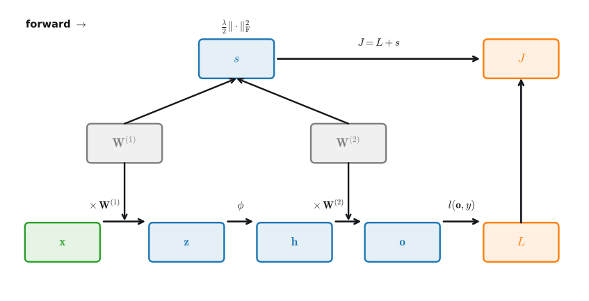
Plotting computational graphs helps us visualize the dependencies of operators and variables within the calculation. Figure 4.3.1 contains the graph associated with the simple network described above, where squares denote variables and circles denote operators. The lower-left corner signifies the input and the upper-right corner is the output. Notice that the directions of the arrows (which illustrate data flow) are primarily rightward and upward.
4.3.3 Backpropagation
Backpropagation refers to the method of calculating the gradient of neural network parameters. In short, the method traverses the network in reverse order, from the output to the input layer, according to the chain rule from calculus (Chapter 25). The algorithm stores any intermediate variables (partial derivatives) required while calculating the gradient with respect to some parameters. Assume that we have functions \(\mathsf{Y}=f(\mathsf{X})\) and \(\mathsf{Z}=g(\mathsf{Y})\), in which the input and the output \(\mathsf{X}, \mathsf{Y}, \mathsf{Z}\) are tensors of arbitrary shapes. By using the chain rule, we can compute the derivative of \(\mathsf{Z}\) with respect to \(\mathsf{X}\) via
\[\frac{\partial \mathsf{Z}}{\partial \mathsf{X}} = \textrm{prod}\left(\frac{\partial \mathsf{Z}}{\partial \mathsf{Y}}, \frac{\partial \mathsf{Y}}{\partial \mathsf{X}}\right). \tag{4.3.6}\]
Here we use the \(\textrm{prod}\) operator to multiply its arguments after the necessary operations, such as transposition and swapping input positions, have been carried out. For vectors, this is straightforward: it is matrix–matrix multiplication. For higher dimensional tensors, we use the appropriate counterpart. The operator \(\textrm{prod}\) hides all the notational overhead; what it computes is made precise as vector–Jacobian products in Section 25.3.
Recall that the simple network with one hidden layer, whose computational graph is in Figure 4.3.1, has parameters \(\mathbf{W}^{(1)}\) and \(\mathbf{W}^{(2)}\). The objective of backpropagation is to calculate the gradients \(\partial J/\partial \mathbf{W}^{(1)}\) and \(\partial J/\partial \mathbf{W}^{(2)}\). To accomplish this, we apply the chain rule and calculate, in turn, the gradient of each intermediate variable and parameter. The order of calculations is reversed relative to those performed in forward propagation, since we need to start with the outcome of the computational graph and work our way towards the parameters. The first step is to calculate the gradients of the objective function \(J=L+s\) with respect to the loss term \(L\) and the regularization term \(s\):
\[\frac{\partial J}{\partial L} = 1 \; \textrm{and} \; \frac{\partial J}{\partial s} = 1. \tag{4.3.7}\]
Next, we compute the gradient of the objective function with respect to the output-layer variable \(\mathbf{o}\) according to the chain rule:
\[ \frac{\partial J}{\partial \mathbf{o}} = \textrm{prod}\left(\frac{\partial J}{\partial L}, \frac{\partial L}{\partial \mathbf{o}}\right) = \frac{\partial L}{\partial \mathbf{o}} \in \mathbb{R}^q. \]
Next, we calculate the gradients of the regularization term with respect to both parameters:
\[\frac{\partial s}{\partial \mathbf{W}^{(1)}} = \lambda \mathbf{W}^{(1)} \; \textrm{and} \; \frac{\partial s}{\partial \mathbf{W}^{(2)}} = \lambda \mathbf{W}^{(2)}. \tag{4.3.8}\]
We can therefore calculate the gradient \(\partial J/\partial \mathbf{W}^{(2)} \in \mathbb{R}^{q \times h}\) of the model parameters closest to the output layer. Using the chain rule yields:
\[\frac{\partial J}{\partial \mathbf{W}^{(2)}}= \textrm{prod}\left(\frac{\partial J}{\partial \mathbf{o}}, \frac{\partial \mathbf{o}}{\partial \mathbf{W}^{(2)}}\right) + \textrm{prod}\left(\frac{\partial J}{\partial s}, \frac{\partial s}{\partial \mathbf{W}^{(2)}}\right)= \frac{\partial J}{\partial \mathbf{o}} \mathbf{h}^\top + \lambda \mathbf{W}^{(2)}. \tag{4.3.9}\]
The “+” in Equation 4.3.9 encodes a general rule: when a variable reaches the output along several paths, its gradient is the sum of the gradients arriving along each path. Here \(\mathbf{W}^{(2)}\) affects \(J\) twice, through the prediction path \(J \leftarrow L \leftarrow \mathbf{o} \leftarrow \mathbf{W}^{(2)}\) and through the regularizer path \(J \leftarrow s \leftarrow \mathbf{W}^{(2)}\), and the two contributions add. Forgetting to accumulate at such forks (overwriting instead of adding) is among the most common bugs in hand-written backward passes.
To obtain the gradient with respect to \(\mathbf{W}^{(1)}\) we need to continue backpropagation along the output layer to the hidden layer. The gradient with respect to the hidden layer output \(\partial J/\partial \mathbf{h} \in \mathbb{R}^h\) is given by
\[ \frac{\partial J}{\partial \mathbf{h}} = \textrm{prod}\left(\frac{\partial J}{\partial \mathbf{o}}, \frac{\partial \mathbf{o}}{\partial \mathbf{h}}\right) = {\mathbf{W}^{(2)}}^\top \frac{\partial J}{\partial \mathbf{o}}. \]
Since the activation function \(\phi\) applies elementwise, calculating the gradient \(\partial J/\partial \mathbf{z} \in \mathbb{R}^h\) of the intermediate variable \(\mathbf{z}\) requires that we use the elementwise multiplication operator, which we denote by \(\odot\):
\[ \frac{\partial J}{\partial \mathbf{z}} = \textrm{prod}\left(\frac{\partial J}{\partial \mathbf{h}}, \frac{\partial \mathbf{h}}{\partial \mathbf{z}}\right) = \frac{\partial J}{\partial \mathbf{h}} \odot \phi'\left(\mathbf{z}\right). \]
Finally, we can obtain the gradient \(\partial J/\partial \mathbf{W}^{(1)} \in \mathbb{R}^{h \times d}\) of the model parameters closest to the input layer. According to the chain rule, we get
\[ \frac{\partial J}{\partial \mathbf{W}^{(1)}} = \textrm{prod}\left(\frac{\partial J}{\partial \mathbf{z}}, \frac{\partial \mathbf{z}}{\partial \mathbf{W}^{(1)}}\right) + \textrm{prod}\left(\frac{\partial J}{\partial s}, \frac{\partial s}{\partial \mathbf{W}^{(1)}}\right) = \frac{\partial J}{\partial \mathbf{z}} \mathbf{x}^\top + \lambda \mathbf{W}^{(1)}. \]
4.3.3.1 A Worked Example
A numerical example makes each backpropagation operation explicit. We apply the local rule that produced every equation above: at each node, multiply the gradient arriving from downstream by the node’s local derivative.
Start with the simplest non-trivial graph, \(e = (a + b)\,c\), evaluated at \(a = 2\), \(b = 1\), \(c = -3\). The forward pass computes the intermediate \(d = a + b = 3\) and then \(e = d\,c = -9\). For the backward pass we seed \(\partial e/\partial e = 1\) and walk back. The multiply node \(e = d\,c\) has local derivatives \(\partial e/\partial d = c = -3\) and \(\partial e/\partial c = d = 3\). The add node \(d = a + b\) has \(\partial d/\partial a = \partial d/\partial b = 1\), so it passes its incoming gradient unchanged to both inputs. Chaining,
\[\frac{\partial e}{\partial a} = \frac{\partial e}{\partial d}\frac{\partial d}{\partial a} = -3,\quad \frac{\partial e}{\partial b} = -3,\quad \frac{\partial e}{\partial c} = 3. \tag{4.3.10}\]
This small graph illustrates the algorithm: add nodes broadcast the upstream gradient unchanged, multiply nodes scale it by the other input. Every backward equation in this section is an instance of this local calculation.
Apply the same calculation to the preceding network, reduced to \(d = h = 2\) inputs and hidden units, \(q = 1\) output, with ReLU activation \(\phi(z) = \max(0, z)\) and (for clarity) no regularization, \(\lambda = 0\). Take
\[ \mathbf{x} = \begin{bmatrix} 1 \\ 2 \end{bmatrix},\quad \mathbf{W}^{(1)} = \begin{bmatrix} 1 & -1 \\ 0 & \phantom{-}1 \end{bmatrix},\quad \mathbf{W}^{(2)} = \begin{bmatrix} 2 & -1 \end{bmatrix},\quad y = 0, \tag{4.3.11}\]
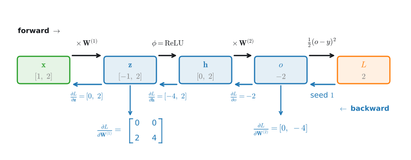
and squared-error loss \(L = \tfrac12 (o - y)^2\). The forward pass gives \(\mathbf{z} = \mathbf{W}^{(1)}\mathbf{x} = [-1,\ 2]^\top\), so \(\mathbf{h} = \phi(\mathbf{z}) = [0,\ 2]^\top\) (the first unit is dead), \(o = \mathbf{W}^{(2)}\mathbf{h} = -2\), and \(L = \tfrac12(-2)^2 = 2\). For the backward pass, \(\partial L/\partial o = o - y = -2\), and then, reading the section’s equations top to bottom,
\[\frac{\partial L}{\partial \mathbf{W}^{(2)}} = \frac{\partial L}{\partial o}\,\mathbf{h}^\top = -2\,[0,\ 2] = [0,\ -4],\]
\[\frac{\partial L}{\partial \mathbf{h}} = {\mathbf{W}^{(2)}}^\top \frac{\partial L}{\partial o} = [-4,\ 2]^\top,\qquad \frac{\partial L}{\partial \mathbf{z}} = \frac{\partial L}{\partial \mathbf{h}} \odot \phi'(\mathbf{z}) = [-4,\ 2]^\top \odot [0,\ 1]^\top = [0,\ 2]^\top, \tag{4.3.12}\]
using \(\phi'(z) = \mathbf{1}[z > 0]\), so the inactive first unit has zero derivative and blocks the gradient. Finally,
\[\frac{\partial L}{\partial \mathbf{W}^{(1)}} = \frac{\partial L}{\partial \mathbf{z}}\,\mathbf{x}^\top = \begin{bmatrix} 0 \\ 2 \end{bmatrix}[1,\ 2] = \begin{bmatrix} 0 & 0 \\ 2 & 4 \end{bmatrix}. \tag{4.3.13}\]
Figure 4.3.2 traces these numbers through the graph, forward in black and backward in blue. Notice that the row of \(\partial L/\partial \mathbf{W}^{(1)}\) feeding the dead unit is entirely zero: no gradient means no learning signal, a concrete instance of the “dying ReLU” we met in Section 4.1. You can confirm every number here in a few lines of automatic differentiation (Section 1.5): rebuild the same tensors with gradient tracking, run the forward pass, sweep back through the graph, and compare against the manually derived gradients. The arithmetic is framework-independent; the frameworks differ only in how they expose the gradients at interior nodes of the graph. PyTorch retains them on request, TensorFlow’s tape can differentiate with respect to any tensor it recorded, JAX differentiates the tail function that consumes the node, and MXNet replays the tail of the graph with the node as an input.
x, y = torch.tensor([1., 2.]), 0
W1 = torch.tensor([[1., -1.], [0., 1.]], requires_grad=True)
W2 = torch.tensor([[2., -1.]], requires_grad=True)
z = W1 @ x
h = torch.relu(z)
o = W2 @ h
for v in (z, h): v.retain_grad()  # keep gradients of non-leaf tensors
L = ((o - y) ** 2).sum() / 2
L.backward()
print(f'L = {L.item()}, dL/dW2 = {W2.grad}, dL/dh = {h.grad}')
print(f'dL/dz = {z.grad}, dL/dW1 =\n{W1.grad}')
L = 2.0, dL/dW2 = tensor([[-0., -4.]]), dL/dh = tensor([-4., 2.])
dL/dz = tensor([0., 2.]), dL/dW1 =
tensor([[0., 0.],
[2., 4.]])x, y = tf.constant([1., 2.]), 0
W1 = tf.Variable([[1., -1.], [0., 1.]])
W2 = tf.Variable([[2., -1.]])
with tf.GradientTape() as tape:
z = tf.linalg.matvec(W1, x)
h = tf.nn.relu(z)
o = tf.linalg.matvec(W2, h)
L = tf.reduce_sum((o - y) ** 2) / 2
# the tape can differentiate with respect to interior tensors directly
dW1, dW2, dz, dh = tape.gradient(L, [W1, W2, z, h])
print(f'L = {L.numpy()}, dL/dW2 = {dW2.numpy()}, dL/dh = {dh.numpy()}')
print(f'dL/dz = {dz.numpy()}, dL/dW1 =\n{dW1.numpy()}')L = 2.0, dL/dW2 = [[-0. -4.]], dL/dh = [-4. 2.]
dL/dz = [-0. 2.], dL/dW1 =
[[-0. -0.]
[ 2. 4.]]x, y = jnp.array([1., 2.]), 0
W1 = jnp.array([[1., -1.], [0., 1.]])
W2 = jnp.array([[2., -1.]])
z, h = W1 @ x, jax.nn.relu(W1 @ x)
loss = lambda W1, W2: ((W2 @ jax.nn.relu(W1 @ x) - y) ** 2).sum() / 2
L, (dW1, dW2) = jax.value_and_grad(loss, argnums=(0, 1))(W1, W2)
# the gradient at an interior node is the gradient of the tail function
# of the graph that consumes it
dh = jax.grad(lambda h: ((W2 @ h - y) ** 2).sum() / 2)(h)
dz = jax.grad(lambda z: ((W2 @ jax.nn.relu(z) - y) ** 2).sum() / 2)(z)
print(f'L = {L}, dL/dW2 = {dW2}, dL/dh = {dh}')
print(f'dL/dz = {dz}, dL/dW1 =\n{dW1}')L = 2.0, dL/dW2 = [[-0. -4.]], dL/dh = [-4. 2.]
dL/dz = [0. 2.], dL/dW1 =
[[0. 0.]
[2. 4.]]x, y = np.array([1., 2.]), 0
W1 = np.array([[1., -1.], [0., 1.]])
W2 = np.array([[2., -1.]])
for v in (W1, W2): v.attach_grad()
with autograd.record():
z = np.dot(W1, x)
h = npx.relu(z)
o = np.dot(W2, h)
L = ((o - y) ** 2).sum() / 2
L.backward()
# the replay below also writes W1.grad and W2.grad, so copy them out first
dW1, dW2 = W1.grad.copy(), W2.grad.copy()
# attach_grad() on an interior node would detach it from the graph, so
# rebuild z and h as leaves and replay the tail of the graph from each
z, h = np.dot(W1, x), npx.relu(np.dot(W1, x))
for v in (z, h): v.attach_grad()
with autograd.record():
Lz = ((np.dot(W2, npx.relu(z)) - y) ** 2).sum() / 2
Lh = ((np.dot(W2, h) - y) ** 2).sum() / 2
Ltail = Lz + Lh
Ltail.backward()
print(f'L = {L}, dL/dW2 = {dW2}, dL/dh = {h.grad}')
print(f'dL/dz = {z.grad}, dL/dW1 =\n{dW1}')L = 2.0, dL/dW2 = [[ 0. -4.]], dL/dh = [-4. 2.]
dL/dz = [-0. 2.], dL/dW1 =
[[0. 0.]
[2. 4.]]Every printed gradient matches the hand computation, down to the zeroed-out row for the dead unit. (The \(-0\) in \(\partial L/\partial \mathbf{W}^{(2)}\) is floating point’s signed zero, an artifact of multiplying \(h_1 = 0\) by the negative upstream gradient; it compares equal to \(0\).)
4.3.3.2 From the Chain Rule to Autograd
A deep learning framework performs the same operations when computing gradients: it records the computational graph during the forward pass, seeds a gradient of \(1\) at the scalar objective, and sweeps the graph in reverse, multiplying the local derivative at each node (our \(\textrm{prod}\)) to accumulate the gradient with respect to every parameter in a single pass. This output-to-input sweep is reverse-mode automatic differentiation, and it is cheap exactly when there are many parameters and one scalar loss, the deep learning regime. We use it throughout the book, and Section 1.5 develops its mechanics, including when the opposite forward mode is preferable. Section 25.3 gives the full theory, expressing both modes as Jacobian products and working out the memory trade-offs they imply.
4.3.4 Training Neural Networks
When training neural networks, forward and backward propagation depend on each other. In particular, for forward propagation, we traverse the computational graph in the direction of dependencies and compute all the variables on its path. These are then used for backpropagation where the compute order on the graph is reversed.
Take the aforementioned simple network as an illustrative example. On the one hand, computing the regularization term Equation 4.3.5 during forward propagation depends on the current values of model parameters \(\mathbf{W}^{(1)}\) and \(\mathbf{W}^{(2)}\). They are given by the optimization algorithm according to backpropagation in the most recent iteration. On the other hand, the gradient calculation for the parameter Equation 4.3.9 during backpropagation depends on the current value of the hidden layer output \(\mathbf{h}\), which is given by forward propagation.
Therefore when training neural networks, once model parameters are initialized, we alternate forward propagation with backpropagation, updating model parameters using gradients given by backpropagation. Note that backpropagation reuses the stored intermediate values from forward propagation to avoid duplicate calculations. One of the consequences is that we need to retain the intermediate values until backpropagation is complete. This is also one of the reasons why training requires significantly more memory than plain prediction. Besides, the size of such intermediate values is roughly proportional to the number of network layers and the batch size. Thus, training deeper networks using larger batch sizes more easily leads to out-of-memory errors.
4.3.5 Summary
Forward propagation sequentially calculates and stores intermediate variables within the computational graph defined by the neural network. It proceeds from the input to the output layer. Backpropagation sequentially calculates and stores the gradients of intermediate variables and parameters within the neural network in the reversed order. When training deep learning models, forward propagation and backpropagation are interdependent, and training requires significantly more memory than prediction.
4.3.6 Exercises
- Jacobian of a layer. The gradient of the scalar \(J\) with respect to \(\mathbf{W}^{(2)} \in \mathbb{R}^{q \times h}\) has the shape of \(\mathbf{W}^{(2)}\). The derivative of the vector \(\mathbf{o} = \mathbf{W}^{(2)} \mathbf{h} \in \mathbb{R}^q\) with respect to \(\mathbf{W}^{(2)}\) is a larger object.
- Give the shape of \(\partial \mathbf{o}/\partial \mathbf{W}^{(2)}\) and the largest number of nonzero entries it can have.
- Evaluate \(\textrm{prod}(\partial J/\partial \mathbf{o}, \partial \mathbf{o}/\partial \mathbf{W}^{(2)})\) entry by entry to recover the term \((\partial J/\partial \mathbf{o})\mathbf{h}^\top\) of Equation 4.3.9. Explain why backpropagation never needs to store \(\partial \mathbf{o}/\partial \mathbf{W}^{(2)}\).
- Hidden-layer bias. Add a bias to the hidden layer of the model described in this section (you do not need to include the bias in the regularization term).
- Draw the corresponding computational graph.
- Derive the forward and backward propagation equations.
- Modified activation. The first hidden unit of the network in Equation 4.3.11 receives the pre-activation \(z_1 = -1\), so the ReLU derivative \(\phi'(z_1) = 0\) blocks the gradient of every weight feeding this unit. Replace the activation of this unit alone by the leaky variant \(\phi_1(z) = \max(0, z) + 0.1 \min(0, z)\); the second unit keeps its ReLU.
- Write the backward equation for \(\partial J/\partial \mathbf{z}\) when hidden unit \(i\) has its own activation \(\phi_i\).
- Redo the forward and backward passes, and give \(\partial L/\partial \mathbf{W}^{(2)}\), \(\partial L/\partial \mathbf{z}\), and \(\partial L/\partial \mathbf{W}^{(1)}\). Which of these gradients differ from the all-ReLU case even though the equations that produce them are unchanged, and why?
- Memory footprint. Train the model described in this section by minibatch stochastic gradient descent on minibatches of \(n\) examples, with input dimension \(d\), \(h\) hidden units, and output dimension \(q\).
- List the forward-pass quantities that a training step must keep until the backward pass has used them. Count their values together with the values of the parameters and of their gradients.
- Prediction can discard each intermediate value as soon as the next operation has consumed it. Count the largest number of values that prediction on the same minibatch holds at any moment.
- For which minibatch sizes \(n\) do the kept forward-pass quantities outnumber the parameters and their gradients together?
- Second derivatives. Automatic differentiation obtains second derivatives by differentiating the backward pass, so the operations of the backward pass become nodes of a larger computational graph. Extend Figure 4.3.1 with the backward-pass nodes that compute \(\partial J/\partial \mathbf{W}^{(1)}\), and mark which forward-pass variables each new node reads.
- Hessian of a ReLU network. ● ReLU has \(\phi''(z) = 0\) for \(z \neq 0\). For the network in Equation 4.3.11, derive the \(4 \times 4\) Hessian of \(L\) with respect to the entries of \(\mathbf{W}^{(1)}\), show that it has rank at most one, and evaluate it at the given values.
- Graph partitioning. Assume that the computational graph is too large for the memory of a single GPU.
- Propose two different strategies for splitting training across two GPUs. For each, state what every GPU stores and what the two GPUs must communicate.
- For each strategy, name one advantage and one disadvantage relative to training on a single GPU with a smaller minibatch.
- [code] Batched backprop. This section’s forward and backward equations process one example \(\mathbf{x}\) at a time.
- Rewrite them to process a minibatch of \(n\) examples, stored as the columns of \(\mathbf{X} \in \mathbb{R}^{d \times n}\), using matrix operations only, with the loss averaged over the batch. Track the shape of every intermediate quantity.
- Implement the batched equations and verify that the resulting gradients match the average of the \(n\) per-example gradients computed by automatic differentiation.
- Forward mode. Backpropagation seeds \(\partial J/\partial J = 1\) at the output and sweeps the graph backward. Forward-mode differentiation instead seeds \(\partial w/\partial w = 1\) at one chosen scalar parameter \(w\) and sweeps forward: each node computes the derivative of its value with respect to \(w\) from the derivatives of its inputs.
- Use forward mode to recompute \(\partial L/\partial \mathbf{W}^{(1)}\) for the network in Equation 4.3.11, one sweep per entry of \(\mathbf{W}^{(1)}\).
- How many sweeps does each mode need to obtain all six parameter gradients of this network? Which factors does forward mode multiply again in every sweep that reverse mode multiplies only once?
- [extended] Autograd engine. ● Build a miniature autograd engine and use it to re-derive the gradients of the network in
Equation 4.3.11.
- Write a scalar
Valueclass that records, for each result, its inputs and the operation that produced it (the computational graph), supporting+,*, andrelu. (Hint: implement__add__and__mul__so that each returns a newValueholding references to its parents and a small function that propagates the gradient one step.) - Implement
backward(): topologically sort the graph, seed the output’s gradient with \(1\), and sweep the nodes in reverse order, letting each node pass its gradient to its parents. Make sure gradients accumulate (+=, not=) when a value is used more than once (the fork rule from Equation 4.3.9). - Reproduce the calculation for Equation 4.3.11 with your engine (unroll the matrix products into scalars), and compare its values of \(\partial L/\partial \mathbf{W}^{(2)}\), \(\partial L/\partial \mathbf{h}\), \(\partial L/\partial \mathbf{z}\), and \(\partial L/\partial \mathbf{W}^{(1)}\) with those derived in this section.
- Consider the chain in which the input \(x\) produces \(y_i = f_i(x)\) for \(i = 1, 2, 3\), the intermediate value \(u = y_1 + y_2 + y_3\), the values \(z_k = g_k(u)\) for \(k = 1, 2, 3\), and the loss \(L = z_1 + z_2 + z_3\). Write \(a_i = f_i'(x)\) and \(b_k = g_k'(u)\). The sum-over-paths view of the chain rule enumerates \(3 \times 3 = 9\) paths from \(x\) to \(L\), each contributing the product \(a_i b_k\). Show that your engine instead computes \((a_1 + a_2 + a_3)(b_1 + b_2 + b_3)\) by accumulating the gradient at \(u\) once, and explain why this sharing is what makes backpropagation affordable in deep networks.
micrograd/engine.py. - Write a scalar