w, x, y, z = 1, 1, -2, 1
# Forward pass: node values
a, b = (w + x + y + z)**2, (w + x - y - z)**2
u, v = (a + b)**2, (a - b)**2
f = (u + v)**2
print('a, b, u, v, f =', a, b, u, v, f)

# Edge derivatives
df_du, df_dv = 2*(u + v), 2*(u + v)
du_da, du_db, dv_da, dv_db = 2*(a + b), 2*(a + b), 2*(a - b), -2*(a - b)
da_dw, db_dw = 2*(w + x + y + z), 2*(w + x - y - z)

# Forward mode: push the dependence on w through the graph
du_dw, dv_dw = du_da*da_dw + du_db*db_dw, dv_da*da_dw + dv_db*db_dw
df_dw = df_du*du_dw + df_dv*dv_dw
print('df/dw =', df_dw)34.3 The Chain Rule on Computational Graphs
Every training step in this book began with one call, backward() or grad, and that one call returned the slope of the loss with respect to every weight. Section 34.2 said what these slopes mean: together they form the gradient, the vector that predicts the effect of any small joint move. It did not say how a program finds a million of them for the price of a few evaluations of the network. The obvious method, nudging one weight and running the network again, needs one run per weight.
The chain rule does much better, and the reason can be stated before any algebra. A network is a long composition of simple functions, and the derivatives with respect to its many weights share most of their work, since every one of them has to pass through the last layer. A formula for the composition hides this sharing. A graph shows it: draw a node for each intermediate value and an edge for each direct dependence. On the graph the chain rule is a sum over paths, and the shared work becomes a choice of how to group the sum. If we group the paths from the output backward, one pass yields the slope with respect to every input. This grouping is backpropagation.
We work the idea out on graphs of scalars that are small enough to compute by hand, with integer values throughout, so that every claim can be checked. The section needs one fact from Section 34.2: near a point, a differentiable function changes by the dot product of the step with its gradient, the linear model Equation 34.2.3. Layers that map vectors to vectors, and the cost of the method on a real network, come in the two sections that follow.
34.3.1 The Chain Rule as a Sum over Paths
34.3.1.1 A Graph of Scalars
Our first example is a toy: four inputs \(w, x, y, z\) flow through intermediate quantities to a scalar output,
\[ \begin{aligned} f(u, v) & = (u+v)^{2}, \\ u(a, b) & = (a+b)^{2}, \qquad v(a, b) = (a-b)^{2}, \\ a(w, x, y, z) & = (w+x+y+z)^{2}, \qquad b(w, x, y, z) = (w+x-y-z)^2. \end{aligned} \tag{34.3.1}\]
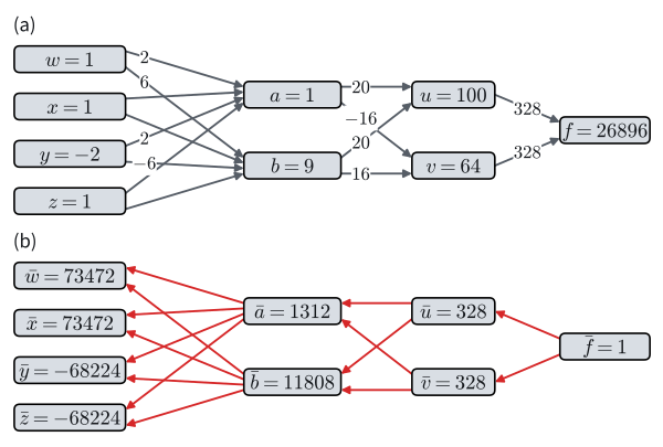
The dependencies form a graph (Figure 34.3.1): each node is a value, and each edge a direct functional dependence. Nothing about the squares is special; they keep the numbers whole. Throughout the section \(f\) denotes the output of the graph at hand.

34.3.1.2 Two Paths through One Step
Take the last composite step, \(f(u(a,b), v(a,b))\), and perturb \(a\) by a small \(\epsilon\). Each intermediate moves by its partial derivative, \(u \to u + \epsilon\frac{\partial u}{\partial a}\) and \(v \to v + \epsilon\frac{\partial v}{\partial a}\). Feeding these moves into the first-order expansion Equation 34.2.3 of \(f\) gives
\[ f\!\left(u + \epsilon\tfrac{\partial u}{\partial a},\, v + \epsilon\tfrac{\partial v}{\partial a}\right) \approx f(u, v) + \epsilon\left[\frac{\partial f}{\partial u}\frac{\partial u}{\partial a} + \frac{\partial f}{\partial v}\frac{\partial v}{\partial a}\right]. \]
The coefficient of \(\epsilon\) is the derivative of the composite with respect to \(a\), and the result is the multivariable chain rule,
\[ \frac{\mathrm{d} f}{\mathrm{d} a} = \frac{\partial f}{\partial u}\frac{\partial u}{\partial a} + \frac{\partial f}{\partial v}\frac{\partial v}{\partial a}. \]
The two kinds of \(d\) are deliberate, and this chapter keeps them apart from here on. The symbol \(\partial\) is reserved for the derivative of one node’s function with respect to one of its arguments, the others held fixed. The total derivative \(\mathrm{d}f/\mathrm{d}a\) lets everything downstream of \(a\) respond. (For an input, the total is the ordinary partial derivative of \(f\) regarded as a function of the inputs alone.) There are two paths by which \(a\) influences \(f\), \(a \to u \to f\) and \(a \to v \to f\). Each path contributes the product of the derivatives along its edges, and the total is the sum over the paths.
The argument is the one-variable proof of the chain rule again (Section 34.1.2): feed the change of the inner functions into the linear model of the outer one. Note, however, that it feeds two simultaneous moves into one linear expansion. That needs \(f\) to be differentiable, not merely to have partial derivatives. For the counterexample \(2xy/(x^2+y^2)\) of Section 34.2.1.2 along the line \(x = y = t\), the rule would predict derivative \(0\) at \(t = 0\) from the two zero partials, yet the function jumps from \(0\) to \(1\) there.
34.3.1.3 Edge Derivatives and Total Derivatives
The rule extends to any graph. Call the edge derivative of a node with respect to one of its parents the partial derivative of the node’s function with respect to that parent, holding its other parents fixed. Then for an output \(f\) and an input \(x\),
\[ \frac{\mathrm{d} f}{\mathrm{d} x} = \sum_{\text{directed paths } x \to \cdots \to f} \;\; \prod_{\text{edges on the path}} (\text{edge derivative}). \tag{34.3.2}\]
Each path multiplies the local rates along its edges, and the paths add. A graph in which one node feeds the output both directly and through a later node shows why edge derivatives must be kept apart from totals. Consider
\[ \begin{aligned} p(x, y) & = x + y, \qquad q(x, y) = x - y, \\ r(p) & = p^2, \qquad s(q) = q^2, \\ f(r, p, s) & = r + p + s. \end{aligned} \tag{34.3.3}\]
The output \(f\) depends on \(r\), on \(s\), and also directly on \(p\), a skip edge (Figure 34.3.2). The input \(y\) reaches \(f\) by three paths, \(y \to p \to r \to f\), \(y \to p \to f\), and \(y \to q \to s \to f\). The edge derivatives are \(\partial f/\partial r = \partial f/\partial p = \partial f/\partial s = 1\), \(\partial r/\partial p = 2p\), \(\partial s/\partial q = 2q\), \(\partial p/\partial y = 1\), and \(\partial q/\partial y = -1\), so
\[ \frac{\mathrm{d} f}{\mathrm{d} y} = \underbrace{1 \cdot 2p \cdot 1}_{y \to p \to r \to f} + \underbrace{1 \cdot 1}_{y \to p \to f} + \underbrace{1 \cdot 2q \cdot (-1)}_{y \to q \to s \to f} = 2p + 1 - 2q = 1 + 4y. \]
Direct substitution, \(f = (x+y)^2 + (x+y) + (x-y)^2\), confirms the sum \(1 + 4y\). At \((x, y) = (1, 2)\), \(p = 3\) and \(q = -1\), and the paths contribute \(6 + 1 + 2 = 9 = 1 + 4 \cdot 2\). The edge derivative \(\partial f/\partial p\) is \(1\), but the total derivative \(\mathrm{d}f/\mathrm{d}p\), through the skip edge and through \(r\), is \(2p + 1 = 7\). Confusing the two is the usual way to get the multivariable chain rule wrong.

The sum over paths is how gradients flow through a network. Architectural choices that open or close paths, such as the gates of an LSTM (Section 12.1) or the skip connections of a residual block (Section 7.4), shape learning by controlling which paths carry gradient.
34.3.2 Backpropagation
As a formula the sum over paths is complete: it gives every derivative of every graph. As an algorithm it is hopeless, because the number of paths grows quickly with depth. A chain of \(m\) stages with two parallel nodes per stage already has \(2^m\) paths from end to end. Luckily the paths share edges, and a product that many paths share needs to be computed only once. The way we group the shared products decides the cost.
34.3.2.1 Forward Mode
We compare two groupings on the four-input function Equation 34.3.1 at \((w, x, y, z) = (1, 1, -2, 1)\). A forward pass evaluates the nodes in order: \(a = 1^2 = 1\), \(b = 3^2 = 9\), \(u = 10^2 = 100\), \(v = (-8)^2 = 64\), and \(f = 164^2 = 26896\). The edge derivatives at these values are
\[ \begin{aligned} \frac{\partial f}{\partial u} = \frac{\partial f}{\partial v} &= 2(u+v) = 328, \\ \frac{\partial u}{\partial a} = \frac{\partial u}{\partial b} &= 2(a+b) = 20, \qquad \frac{\partial v}{\partial a} = 2(a-b) = -16, \qquad \frac{\partial v}{\partial b} = -2(a-b) = 16, \\ \frac{\partial a}{\partial w} = \frac{\partial a}{\partial x} = \frac{\partial a}{\partial y} = \frac{\partial a}{\partial z} &= 2(w+x+y+z) = 2, \\ \frac{\partial b}{\partial w} = \frac{\partial b}{\partial x} = 2(w+x-y-z) &= 6, \qquad \frac{\partial b}{\partial y} = \frac{\partial b}{\partial z} = -6. \end{aligned} \]
Every edge derivative is a number we can compute locally, from the values of a node and its parents.
The four paths from \(w\) to \(f\) go through \(a\) or \(b\) and then through \(u\) or \(v\). Pushing \(w\) forward through the graph collects them as
\[ \begin{aligned} \frac{\mathrm{d} f}{\mathrm{d} w} &= \frac{\partial f}{\partial u}\Bigl(\frac{\partial u}{\partial a}\frac{\partial a}{\partial w} + \frac{\partial u}{\partial b}\frac{\partial b}{\partial w}\Bigr) + \frac{\partial f}{\partial v}\Bigl(\frac{\partial v}{\partial a}\frac{\partial a}{\partial w} + \frac{\partial v}{\partial b}\frac{\partial b}{\partial w}\Bigr) \\ &= 328\,(20\cdot 2 + 20 \cdot 6) + 328\,(-16 \cdot 2 + 16 \cdot 6) = 328 \cdot 224 = 73472. \end{aligned} \]
The bracketed sums are \(\mathrm{d}u/\mathrm{d}w = 160\) and \(\mathrm{d}v/\mathrm{d}w = 64\), the total derivatives of the intermediates with respect to \(w\). Carrying the dependence on one input forward through the graph in this way is called forward mode. In plain Python:
a, b, u, v, f = 1 9 100 64 26896
df/dw = 73472
Forward mode returns \(\mathrm{d}f/\mathrm{d}w = 73472\), but nothing in it can be reused for \(x\), \(y\), or \(z\): \(\mathrm{d}u/\mathrm{d}w\) and \(\mathrm{d}v/\mathrm{d}w\) belong to \(w\) alone. Training needs the derivative of one loss with respect to every parameter, and this grouping computes them one input at a time.
34.3.2.2 Adjoints and the Backward Pass
The remedy is to keep the output fixed instead of the input. Forward mode asked, for one input, how every later node responds to it. We now ask, for the one output, how it responds to every earlier node. The adjoint \(\bar{n}\) of a node \(n\) is the total derivative \(\mathrm{d}f/\mathrm{d}n\) of the output with respect to that node: the sum, over all paths from \(n\) to \(f\), of the products of the edge derivatives. Every such path leaves \(n\) through one of its children \(c\), the nodes that use \(n\) directly, and the paths from \(c\) onward sum to \(\bar{c}\). Grouping the sum Equation 34.3.2 by this first edge turns it into a recursion,
\[ \bar{f} = 1, \qquad \bar{n} = \sum_{\text{children } c \text{ of } n} \bar{c}\,\frac{\partial c}{\partial n}, \tag{34.3.4}\]
in which only edge derivatives and the adjoints of later nodes appear. Starting from \(\bar f = 1\) and visiting the nodes from the output backward, each adjoint is ready when it is needed. In the skip-edge graph Equation 34.3.3 the recursion gives \(\bar r = 1\) and \(\bar p = \bar r \cdot 2p + \bar f \cdot 1 = 7\), the total found there. For the four-input graph:
- \(\bar{u} = \bar{v} = 328\);
- \(\bar{a} = \bar{u}\cdot 20 + \bar{v}\cdot(-16) = 1312\) and \(\bar{b} = \bar{u}\cdot 20 + \bar{v}\cdot 16 = 11808\);
- \(\bar{w} = \bar{x} = \bar{a}\cdot 2 + \bar{b}\cdot 6 = 73472\) and \(\bar{y} = \bar{z} = \bar{a}\cdot 2 - \bar{b}\cdot 6 = -68224\).
One backward pass gives the derivatives with respect to all four inputs (Figure 34.3.3). The code reuses the edge derivatives of the forward-mode cell.
da_dy, db_dy = 2*(w + x + y + z), -2*(w + x - y - z)  # also for x, z
# Backward pass: adjoints from the output toward the inputs
u_bar, v_bar = df_du, df_dv
a_bar = u_bar*du_da + v_bar*dv_da
b_bar = u_bar*du_db + v_bar*dv_db
print(f'adjoints: u {u_bar}, v {v_bar}, a {a_bar}, b {b_bar}')
w_bar = a_bar*da_dw + b_bar*db_dw  # x enters a, b like w
y_bar = a_bar*da_dy + b_bar*db_dy  # z enters a, b like y
print('gradient:', {'w': w_bar, 'x': w_bar, 'y': y_bar, 'z': y_bar})
adjoints: u 328, v 328, a 1312, b 11808
gradient: {'w': 73472, 'x': 73472, 'y': -68224, 'z': -68224}The derivatives with respect to \(w\) and \(x\) agree, and so do those with respect to \(y\) and \(z\), because \(f\) depends on its inputs only through \(w + x\) and \(y + z\).
Counting multiplications shows the saving. Forward mode needs six per input (two each for \(\mathrm{d}u/\mathrm{d}w\), \(\mathrm{d}v/\mathrm{d}w\), and \(\mathrm{d}f/\mathrm{d}w\)), 24 for four inputs. The backward pass needs four for \(\bar a\) and \(\bar b\) and then two per input, 12 in all: it does the work on the shared part of the graph once. A factor of two is nothing to boast of. But the saving grows with the number of inputs: each further input costs forward mode a whole pass and the backward pass two multiplications.
34.3.2.3 Backpropagation in a Framework
Computing derivatives from the output back toward the inputs is backpropagation (Rumelhart et al. 1986), which Section 4.3 applies to a multilayer perceptron. Each framework’s automatic differentiation runs the same two passes: it records values and edge derivatives on the way forward and accumulates adjoints on the way back. Here it is on the same four inputs.
wxyz = torch.tensor([1., 1., -2., 1.], requires_grad=True)
w, x, y, z = wxyz
a, b = (w + x + y + z)**2, (w + x - y - z)**2
u, v = (a + b)**2, (a - b)**2
f = (u + v)**2
f.backward()  # one backward pass
print(wxyz.grad)
tensor([ 73472., 73472., -68224., -68224.])wxyz = tf.Variable([1., 1., -2., 1.])
with tf.GradientTape() as t:
w, x, y, z = tf.unstack(wxyz)
a, b = (w + x + y + z)**2, (w + x - y - z)**2
u, v = (a + b)**2, (a - b)**2
f = (u + v)**2
print(t.gradient(f, wxyz).numpy()) # one backward pass[ 73472. 73472. -68224. -68224.]def f_graph(wxyz):
w, x, y, z = wxyz
a, b = (w + x + y + z)**2, (w + x - y - z)**2
u, v = (a + b)**2, (a - b)**2
return (u + v)**2
print(jax.grad(f_graph)(jnp.array([1., 1., -2., 1.]))) # one backward pass[ 73472. 73472. -68224. -68224.]wxyz = mnp.array([1., 1., -2., 1.])
wxyz.attach_grad()
with autograd.record():
w, x, y, z = wxyz[0], wxyz[1], wxyz[2], wxyz[3]
a, b = (w + x + y + z)**2, (w + x - y - z)**2
u, v = (a + b)**2, (a - b)**2
f = (u + v)**2
f.backward() # one backward pass
print(wxyz.grad)[ 73472. 73472. -68224. -68224.]The library returns \((73472, 73472, -68224, -68224)\), the adjoints of our hand computation. The agreement is exact, not approximate: all the numbers involved are integers below \(2^{24}\), which single precision represents without rounding.
Every node here was a scalar, and we counted multiplications on a graph that fits on a napkin. A layer of a network maps a vector to a vector. Its edge derivatives are matrices, and the order in which matrices are multiplied matters far more than the order of numbers. Section 34.4 takes that step.
34.3.3 Summary
The derivative of an output with respect to an input is the sum, over the paths between them, of the products of the edge derivatives. The adjoint of a node, the total derivative of the output with respect to it, collects all paths leaving the node. Grouping them by their first edge gives a recursion that, run from the output backward, yields every adjoint in one pass. This is backpropagation. Carrying one input forward instead gives that input’s derivative alone, so a loss with many inputs is differentiated backward.
34.3.4 Exercises
[code] Backward pass for two tanh units. A network with one input \(x\), two hidden units, and one output computes, for a target \(t\),
\[h_i = \tanh(w_i x + b_i) \quad (i = 1, 2), \qquad f = v_1 h_1 + v_2 h_2, \qquad \ell = \tfrac12 (f - t)^2.\]
- Draw the dependency graph of \(\ell\). In plain Python, write a forward pass that stores every intermediate value and a backward pass that returns the partial derivatives of \(\ell\) with respect to all six parameters \(w_1, b_1, w_2, b_2, v_1, v_2\). Check them against automatic differentiation at \(x = 1.5\), \(t = 0.5\), and \((w_1, b_1, w_2, b_2, v_1, v_2) = (0.5, 0, -1, 0.2, 1, -0.5)\). Which intermediate derivative does every one of the six partials reuse?
- Set \(w_1 = 5\) and \(x = 2\), keeping the other values. Compute \(\partial \ell / \partial w_1\) with the plain-Python backward pass and explain its size from the product of edge derivatives along its path. Compare it with the value that automatic differentiation returns in single precision, and explain the difference. What does this imply for training a unit whose pre-activation is large?
- Set \(w_1 = w_2\), \(b_1 = b_2\), and \(v_1 = v_2\). Show from the backward pass that both units receive identical gradients, so that gradient descent keeps them identical at every step. What does this imply for the initialization of hidden units?
Paths through a residual stack. ● In a one-dimensional model of the residual networks of Section 7.4, scalar blocks compute \(x_{l+1} = x_l + g_l(x_l)\) for \(l = 0, \ldots, m-1\) with differentiable functions \(g_l\).
- Use the chain rule to write \(\partial x_m / \partial x_0\) as a product of \(m\) factors.
- Expand the product and match each term to a directed path from \(x_0\) to \(x_m\) in the dependency graph. How many paths are there, and how many of them pass through exactly \(k\) of the functions \(g_l\)? Compare the number of paths with the number of multiplications that a backward pass needs to compute \(\partial x_m / \partial x_0\).
- For a trained network of \(m = 54\) residual blocks, Veit et al. (2016) found that almost all of the gradient flows along the paths through \(5\) to \(17\) blocks. What fraction of all paths are these? Now assume that \(g_l'(x_l) = c > 0\) for every block. Which value of \(c\) makes the paths through about \(11\) blocks contribute the most to \(\partial x_m / \partial x_0\), and what share of the derivative do the paths through \(5\) to \(17\) blocks then carry?
[code] Gradient checks in single precision. ● A gradient check compares a backward pass with the central difference \(\bigl(f(w + h, x, y, z) - f(w - h, x, y, z)\bigr) / (2h)\). Let \(f\) be the function of Equation 34.3.1, whose exact partial derivative at \((w, x, y, z) = (1, 1, -2, 1)\) is \(\partial f / \partial w = 73472\).
- Implement \(f\) in NumPy and compute the central difference at this point for \(h = 10^{-1}, 10^{-2}, \ldots, 10^{-12}\), once in
float64and once infloat32. Plot the relative error against \(h\) on log-log axes for both precisions, and read off the best \(h\) and the smallest relative error of each. - The error of the central difference is a truncation part of order \(h^2\) plus a rounding part of order \(\varepsilon_{\textrm{mach}} |f| / h\), where the machine epsilon \(\varepsilon_{\textrm{mach}}\) is about \(2.2 \times 10^{-16}\) for
float64and \(1.2 \times 10^{-7}\) forfloat32. By which factors should the best \(h\) and the smallest relative error change fromfloat64tofloat32? Compare the predicted factors with the plot. - Which tolerance on the relative error can a
float32gradient check use without rejecting a correct backward pass? Why are gradient checks run in double precision? - Why does the
float32estimate become exactly zero for the smallest values of \(h\)?
- Implement \(f\) in NumPy and compute the central difference at this point for \(h = 10^{-1}, 10^{-2}, \ldots, 10^{-12}\), once in