import math
import torch
from torch import nn5.3 Initialization
Every parameter in a network has a value before training starts: a fully connected layer mapping 512 inputs to 256 outputs brings a \(256 \times 512\) weight matrix filled with random numbers. Section 4.4 explains why the scale of those numbers decides whether a deep network trains at all, and derives the Xavier (Glorot and Bengio 2010) and He (He et al. 2015) schemes that keep signal variance stable across layers. This section examines library defaults, applies explicit schemes to a model or submodule, introduces initialization rules used in deep residual and Transformer architectures, and implements custom initializers.
import math
import tensorflow as tf
import math
import jax
from jax import numpy as jnp
from flax import nnximport math
from mxnet import init, np, npx
from mxnet.gluon import nn
npx.set_np()5.3.1 Defaults and When to Override Them
Default initializers are suitable for standard library layers at ordinary depths. Inspect or override them when activation functions, residual depth, custom parameters, or reproduction of a published model impose a specific scaling rule.
PyTorch initializes an nn.Linear the moment it is constructed: weight and bias are both drawn from the uniform distribution \(U(-b, b)\) with \(b = 1/\sqrt{n_\textrm{in}}\), where \(n_\textrm{in}\) is the number of input features. (The documentation describes the weight rule as a variant of He initialization, kaiming_uniform_ with a=math.sqrt(5); the algebra collapses to the bound above.) A uniform distribution on \([-b, b]\) has standard deviation \(b/\sqrt{3}\), so a fresh layer can verify both claims:
Keras attaches no numbers at construction either: Dense(256) fixes only the output width, and the kernel comes into existence at build time, when the layer first learns its input shape (every Keras layer is lazy in the sense of Section 5.1.4). The build draws Glorot uniform, the Xavier scheme of Section 4.4.2.2 in its uniform variant: the kernel comes from \(U(-b, b)\) with \(b = \sqrt{6/(n_\textrm{in} + n_\textrm{out})}\), and the bias starts at zero. A uniform distribution on \([-b, b]\) has standard deviation \(b/\sqrt{3}\), so a fresh layer can verify all three claims:
NNX creates parameters when nnx.Linear is constructed, using the explicit input width to determine fan-in. Its default is LeCun normal: the weight comes from a normal distribution with standard deviation \(1/\sqrt{n_\textrm{in}}\), truncated so that no entry lands in the far tails (the initializer rescales after clipping to keep the standard deviation on target, which puts the hard bound near \(2.3\) standard deviations), and the bias starts at zero. A fresh layer can verify both claims:
Gluon separates construction from initialization: nn.Dense(256) carries no numbers until you call initialize(), and when the input width is left unspecified even that call only records your choice, with the draw deferred to the first forward pass (Section 5.1.4). What it draws is the legacy exception in the table below: every weight comes from \(U(-0.07, 0.07)\) regardless of the layer’s shape, a fixed constant rather than a fan-aware bound, and the bias starts at zero. A uniform distribution on \([-b, b]\) has standard deviation \(b/\sqrt{3}\), so a fresh layer can verify all three claims (passing in_units pins the input width, so nothing is deferred here):
torch.manual_seed(0)
layer = nn.Linear(512, 256)
bound = 1 / math.sqrt(layer.in_features)
w = layer.weight
print(f'range [{w.min():.4f}, {w.max():.4f}], predicted bound {bound:.4f}')
print(f'std {w.std():.4f}, predicted {bound / math.sqrt(3):.4f}')
range [-0.0442, 0.0442], predicted bound 0.0442
std 0.0255, predicted 0.0255tf.keras.utils.set_random_seed(0)
layer = tf.keras.layers.Dense(256)
layer.build((None, 512))
w = layer.kernel.numpy()
bound = math.sqrt(6 / (512 + 256))
print(f'range [{w.min():.4f}, {w.max():.4f}], predicted bound {bound:.4f}')
print(f'std {w.std():.4f}, predicted {bound / math.sqrt(3):.4f}')
print(f'bias all zero: {bool((layer.bias.numpy() == 0).all())}')range [-0.0884, 0.0884], predicted bound 0.0884
std 0.0511, predicted 0.0510
bias all zero: Truelayer = nnx.Linear(512, 256, rngs=nnx.Rngs(0))
w = layer.kernel
print(f'std {w.std():.4f}, predicted {1 / math.sqrt(512):.4f}')
print(f'max |w| {jnp.abs(w).max():.4f}, '
f'bias all zero: {bool((layer.bias == 0).all())}')std 0.0443, predicted 0.0442
max |w| 0.1005, bias all zero: Truenp.random.seed(0)
layer = nn.Dense(256, in_units=512)
layer.initialize()
w = layer.weight.data()
print(f'range [{float(w.min()):.4f}, {float(w.max()):.4f}], '
f'predicted bound 0.0700')
print(f'std {float(w.std()):.4f}, predicted {0.07 / math.sqrt(3):.4f}')
print(f'bias all zero: {bool((layer.bias.data() == 0).all())}')range [-0.0700, 0.0700], predicted bound 0.0700
std 0.0404, predicted 0.0404
bias all zero: TrueOther libraries make different but equally fan-aware choices, with one legacy exception:
| Library | Default for a dense layer’s weight |
|---|---|
| PyTorch | \(U(-1/\sqrt{n_\textrm{in}},\, 1/\sqrt{n_\textrm{in}})\), bias likewise |
| Flax (JAX) | LeCun normal: truncated normal, std \(1/\sqrt{n_\textrm{in}}\); zero bias |
| Keras (TensorFlow) | Glorot uniform: \(U(\pm\sqrt{6/(n_\textrm{in} + n_\textrm{out})})\); zero bias |
| MXNet Gluon | \(U(-0.07, 0.07)\), not fan-aware, so override it; zero bias |
When should you override? Four situations recur: a deep network without normalization layers, where variance compounds across depth (we demonstrate this below); parameters you created by hand, since nn.Parameter(torch.empty(...)) contains whatever bytes the allocator happened to return; reproducing a paper whose results depend on its initialization recipe; and architecture-specific corrections such as the residual scaling later in this section. Note that the defaults are computed from fan-in at construction time; a lazy layer (Section 5.1.4) has no fan-in until its first forward pass, so it runs the same rule at materialization instead.
When should you override? Four situations recur: a deep network without normalization layers, where variance compounds across depth (we demonstrate this below); reproducing a paper whose results depend on its initialization recipe; architecture-specific corrections such as the residual scaling later in this section; and parameters you create by hand, where Keras quietly substitutes a default of its own, since add_weight falls back to Glorot uniform unless you pass an initializer, a sensible scale for a weight matrix and generally unsuitable for parameters with other roles. No additional construction-time rule is needed: fan-in and fan-out are read off the input shape when build runs.
When should you override? Four situations recur: a deep network without normalization layers, where variance compounds across depth (we demonstrate this below); reproducing a paper whose results depend on its initialization recipe; architecture-specific corrections such as the residual scaling later in this section; and parameters you create by hand, though here NNX forces the choice on you: construct the value explicitly and wrap it in nnx.Param. NNX layers receive their input and output widths in the constructor, and their initializers run there as well; no later init pass infers fan-in from the first input.
When should you override? Here the first candidate is the default itself: \(\pm 0.07\) was tuned for the hidden widths of an earlier era and ignores fan-in, so a layer much wider than those starts with too much variance, a much narrower one with too little, and either error compounds across depth by the analysis of Section 4.4. Beyond that, the usual situations recur: a deep network without normalization layers, where variance compounds even when each layer is right (we demonstrate this below); reproducing a paper whose results depend on its initialization recipe; and architecture-specific corrections such as the residual scaling later in this section. Deferred initialization changes the timing: with the input width unspecified, initialize() merely records which initializer to use, and the draw happens at the first forward pass, once the layer knows its fan-in.
5.3.2 Applying Initializers
To impose a scheme we do not touch layers one at a time. net.apply(fn) walks the module tree of Section 5.1 and calls fn on every submodule, children first. The function inspects each module’s type and decides what, if anything, to do with it. The routines in torch.nn.init follow PyTorch’s convention that a trailing underscore means in place: nn.init.normal_(w) overwrites w rather than returning a fresh tensor. In place is what we want here, since the parameter must remain the same tensor object the module registered; replacing it would leave net.parameters() and any existing optimizer pointing at the old one.
To impose a scheme we declare it where the layer is declared: every Keras layer accepts kernel_initializer and bias_initializer arguments, each an object mapping a shape and dtype to a tensor, and tf.keras.initializers supplies the standard menu (the string 'zeros' names the same object as tf.keras.initializers.Zeros()). The arguments are stored at construction and run at build time, so they wait for lazy shapes automatically. That covers models you are about to build. The second route, for a model that already exists, rests on the fact that a kernel is a mutable variable: iterate over model.layers, decide by type what to do with each layer, and overwrite the kernels you select in place with assign. We show both, starting with constructor arguments.
NNX affine layers such as Linear and Conv accept kernel_init and bias_init, each a function (key, shape, dtype) -> array, and nnx.initializers supplies the standard menu. These functions run in the constructor. For a model that already exists, we can walk its modules and assign new values to selected parameters. For a parameter in a custom module, call an initializer directly and wrap its result in nnx.Param. We show the first two routes here.
To impose a scheme we hand an Initializer object to the model: net.initialize(init=..., force_reinit=True) walks every parameter of the block tree of Section 5.1 and runs the initializer on it (force_reinit lifts the guard against silently clobbering a model that already has values). The object is a default, not a decree: a parameter constructed with its own initializer keeps it, and every Dense bias is constructed with zeros, which is why the normal draw below leaves the biases at zero. Dispatching by layer type, the pattern PyTorch users write, is possible (iterate over net and test isinstance), but Gluon’s native unit of selection is the subtree: every block, and every individual parameter, has an initialize method of its own. We show both, starting with the whole net.
net = nn.Sequential(nn.Linear(4, 8), nn.ReLU(), nn.Linear(8, 1))

def init_normal(module):
    if isinstance(module, nn.Linear):
        nn.init.normal_(module.weight, mean=0, std=0.01)
        nn.init.zeros_(module.bias)

net.apply(init_normal)
net[0].weight.data[0], net[0].bias.data[0]
(tensor([ 1.3090e-02, 7.2679e-03, -8.8525e-05, 9.0255e-03]), tensor(0.))init_normal = tf.keras.initializers.RandomNormal(stddev=0.01)
net = tf.keras.Sequential([
tf.keras.layers.Dense(8, kernel_initializer=init_normal,
bias_initializer='zeros'),
tf.keras.layers.ReLU(),
tf.keras.layers.Dense(1, kernel_initializer=init_normal,
bias_initializer='zeros')])
X = tf.ones((2, 4))
net(X)
net.layers[0].kernel[:, 0].numpy(), net.layers[0].bias[0].numpy()(array([ 0.01419753, 0.01572837, -0.02287325, -0.00140878], dtype=float32),
np.float32(0.0))init_normal = nnx.initializers.normal(0.01)
net = nnx.Sequential(
nnx.Linear(4, 8, kernel_init=init_normal,
bias_init=nnx.initializers.zeros, rngs=nnx.Rngs(0)),
nnx.relu,
nnx.Linear(8, 1, kernel_init=init_normal,
bias_init=nnx.initializers.zeros, rngs=nnx.Rngs(1)))
net.layers[0].kernel[:, 0], net.layers[0].bias[0](Array([0.01004014, 0.01661628, 0.00595053, 0.00908357], dtype=float32),
Array(0., dtype=float32))net = nn.Sequential()
net.add(nn.Dense(8, activation='relu'))
net.add(nn.Dense(1))
net.initialize(init=init.Normal(sigma=0.01))
X = np.ones((2, 4))
net(X) # the input width was deferred, so the draw happens here
net[0].weight.data()[0], net[0].bias.data()[0](array([ 0.00490368, 0.00765541, -0.00184343, 0.00680209]), array(0.))The isinstance dispatch is what makes the pattern compose: one function can treat nn.Linear, nn.Conv2d, and nn.Embedding differently, and it silently skips containers and activations. Because apply runs on any subtree, we can also mix schemes per block. Below we give the first layer Xavier initialization (Section 4.4.2.2) and set the last to a constant, a poor idea for training by the symmetry argument of Section 4.4, but it makes the mechanics visible:
Mixing schemes per block needs no dispatch while the model is under construction: each layer names its own initializer, so the choice sits exactly where the layer is declared. Below we give the first layer Xavier initialization (Section 4.4.2.2), which Keras spells GlorotUniform after its author, and set the last to a constant, a poor idea for training by the symmetry argument of Section 4.4, but it makes the mechanics visible:
Mixing schemes per block needs no dispatch at all: each layer names its own initializer, so the choice sits exactly where the layer is declared. Below we give the first layer Xavier initialization (Section 4.4.2.2) and set the last to a constant, a poor idea for training by the symmetry argument of Section 4.4, but it makes the mechanics visible:
Mixing schemes per block is initialize on the subtree: net[0] is a block and net[0].weight is a parameter, and both accept an initializer directly, with force_reinit=True because we are overwriting live values. Below we give the first layer Xavier initialization (Section 4.4.2.2) and set the second to a constant, a poor idea for training by the symmetry argument of Section 4.4, but it makes the mechanics visible:
def init_xavier(module):
    if isinstance(module, nn.Linear):
        nn.init.xavier_uniform_(module.weight)

def init_42(module):
    if isinstance(module, nn.Linear):
        nn.init.constant_(module.weight, 42)

net[0].apply(init_xavier)
net[2].apply(init_42)
net[0].weight.data[0], net[2].weight.data
(tensor([ 0.6055, -0.2622, -0.1840, 0.2908]),
tensor([[42., 42., 42., 42., 42., 42., 42., 42.]]))net = tf.keras.Sequential([
tf.keras.layers.Dense(
8, kernel_initializer=tf.keras.initializers.GlorotUniform()),
tf.keras.layers.ReLU(),
tf.keras.layers.Dense(
1, kernel_initializer=tf.keras.initializers.Constant(42.0))])
net(X)
net.layers[0].kernel[:, 0].numpy(), net.layers[2].kernel[:, 0].numpy()(array([ 0.22517478, -0.18920076, 0.62674755, 0.11356837], dtype=float32),
array([42., 42., 42., 42., 42., 42., 42., 42.], dtype=float32))net = nnx.Sequential(
nnx.Linear(4, 8, kernel_init=nnx.initializers.xavier_uniform(),
rngs=nnx.Rngs(0)), nnx.relu,
nnx.Linear(8, 1, kernel_init=nnx.initializers.constant(42.0),
rngs=nnx.Rngs(1)))
net.layers[0].kernel[:, 0], net.layers[2].kernel(Array([0.48410526, 0.63880914, 0.3169195 , 0.4499392 ], dtype=float32),
Param( # 8 (32 B)
value=Array([[42.],
[42.],
[42.],
[42.],
[42.],
[42.],
[42.],
[42.]], dtype=float32)
))net[0].weight.initialize(init=init.Xavier(), force_reinit=True)
net[1].initialize(init=init.Constant(42), force_reinit=True)
net[0].weight.data()[0], net[1].weight.data()(array([ 0.37153655, -0.47844273, -0.4485028 , -0.5750185 ]),
array([[42., 42., 42., 42., 42., 42., 42., 42.]]))This pattern defines the relevant API. Later chapters package it as helper functions, init_cnn for convolutional networks and init_seq2seq for encoder-decoder models, but each is just a function like init_normal handed to apply.
The second route re-initializes a model that already exists. The loop below is the whole mechanism: iterate model.layers, dispatch with isinstance so that activations and anything else without a kernel are skipped, and assign a fresh draw into each kernel. assign overwrites the variable’s buffer in place, which is what we want, since the parameter must remain the same variable the model tracks and any existing optimizer updates. The function repairs the constant-42 network from the previous cell; biases pass through untouched:
The second route walks the existing object graph. nnx.iter_modules yields each child with its path, and one fresh key per matching layer keeps the draws independent. The function below re-draws every linear kernel of the constant-42 network; biases pass through untouched:
There is no second route to learn, because force_reinit=True already is the route for a model with live values: the two cells above re-initialized the same network three times. Whole net, block, or single parameter, the call is the same, and nothing else is needed.
def reinit(model, init):
    for layer in model.layers:
        if isinstance(layer, tf.keras.layers.Dense):
            layer.kernel.assign(init(layer.kernel.shape))

reinit(net, tf.keras.initializers.GlorotUniform(seed=1))
net.layers[2].kernel[:3]
<tf.Tensor: shape=(3, 1), dtype=float32, numpy=
array([[ 0.6180687 ],
[-0.06535196],
[ 0.16377491]], dtype=float32)>def reinit(model, key, init_fn):
layers = [m for _, m in nnx.iter_modules(model)
if isinstance(m, nnx.Linear)]
for layer, subkey in zip(layers, jax.random.split(key, len(layers))):
layer.kernel[...] = init_fn(
subkey, layer.kernel.shape, layer.kernel.dtype)
reinit(net, jax.random.key(1), nnx.initializers.xavier_uniform())
net.layers[2].kernel[:3]Array([[-0.15734486],
[ 0.0798452 ],
[-0.4529283 ]], dtype=float32)5.3.3 Truncation, Depth Scaling, and Zero Initialization
Xavier and He set the variance of a single layer. The schemes below, standard in transformer codebases, adjust what happens in the distribution’s tails, across depth, and at a block’s start.
5.3.3.1 Truncated Normals
A Gaussian gets the variance right, but its tails are unbounded. That is harmless for one draw, while at scale a far-tail value is a near-certainty: among the \(10^8\) weights of a BERT-sized model, dozens land beyond five standard deviations. Large draws also consume disproportionate dynamic range once a model is cast to low precision (Section 5.5). BERT and implementations in the ViT lineage use truncated-normal initialization (Devlin et al. 2018; Dosovitskiy et al. 2021): the tails are cut off at a fixed multiple of the nominal standard deviation. Raw truncated-normal initializers do not necessarily restore the variance removed with the tails; fan-aware variance-scaling initializers often do.
nn.init.trunc_normal_ takes absolute cutoffs a and b (defaulting to \(\pm 2\), which means \(\pm 2\sigma\) only when std=1), so a clip at two standard deviations must state them explicitly:
tf.keras.initializers.TruncatedNormal fixes its cutoff at two standard deviations: draws landing outside the bound are discarded and redrawn, and no rescaling follows. Truncation also backs the fan-aware factory behind HeNormal and its relatives, which draws a truncated normal and then rescales it so the standard deviation lands on target despite the missing tails:
nnx.initializers.truncated_normal states its cutoffs in units of the standard deviation (lower=-2.0, upper=2.0 by default), so the clip at two standard deviations is what you get with no extra arguments. Truncation is the house preference throughout Flax: the variance_scaling factory behind lecun_normal, xavier_normal, and he_normal draws its normal variants truncated as well.
mxnet.init ships no truncated normal; the library does not provide this scheme. We therefore use the custom initializer interface introduced below: an initializer is a subclass of init.Initializer that fills an array inside its _init_weight method, so the missing entry costs a dozen lines. We draw normal values and redraw every entry that lands outside two standard deviations until none does, the same discard-and-redraw semantics as Keras, and keep the drawing function separate so it can double as the demonstration:
torch.manual_seed(0)
w = torch.empty(1000, 1000)
nn.init.normal_(w, std=0.02)
print(f'normal:    std {w.std():.4f}, max weight {w.abs().max():.4f}')
nn.init.trunc_normal_(w, std=0.02, a=-0.04, b=0.04)
print(f'truncated: std {w.std():.4f}, max weight {w.abs().max():.4f}')
normal: std 0.0200, max weight 0.0952
truncated: std 0.0176, max weight 0.0400init = tf.keras.initializers.RandomNormal(stddev=0.02, seed=0)
w = init((1000, 1000)).numpy()
print(f'normal: std {w.std():.4f}, max weight {abs(w).max():.4f}')
init = tf.keras.initializers.TruncatedNormal(stddev=0.02, seed=0)
w = init((1000, 1000)).numpy()
print(f'truncated: std {w.std():.4f}, max weight {abs(w).max():.4f}')normal: std 0.0200, max weight 0.1046
truncated: std 0.0176, max weight 0.0400key = jax.random.key(0)
w = nnx.initializers.normal(stddev=0.02)(key, (1000, 1000))
print(f'normal: std {w.std():.4f}, max weight {jnp.abs(w).max():.4f}')
w = nnx.initializers.truncated_normal(stddev=0.02)(key, (1000, 1000))
print(f'truncated: std {w.std():.4f}, max weight {jnp.abs(w).max():.4f}')normal: std 0.0200, max weight 0.0929
truncated: std 0.0176, max weight 0.0400def trunc_normal(sigma, shape):
w = np.random.normal(0, sigma, shape)
tails = np.abs(w) > 2 * sigma
while bool(tails.any()):
w = np.where(tails, np.random.normal(0, sigma, shape), w)
tails = np.abs(w) > 2 * sigma
return w
class TruncatedNormal(init.Initializer):
def __init__(self, sigma=0.02):
super().__init__(sigma=sigma)
self.sigma = sigma
def _init_weight(self, name, arr):
arr[:] = trunc_normal(self.sigma, arr.shape)
np.random.seed(0)
w = np.random.normal(0, 0.02, (1000, 1000))
print(f'normal: std {float(w.std()):.4f}, '
f'max weight {float(np.abs(w).max()):.4f}')
w = trunc_normal(0.02, (1000, 1000))
print(f'truncated: std {float(w.std()):.4f}, '
f'max weight {float(np.abs(w).max()):.4f}')normal: std 0.0200, max weight 0.0919
truncated: std 0.0176, max weight 0.0400A million plain-normal draws produce entries near \(5\sigma = 0.1\); the truncated version guarantees \(|w| \leq 0.04\). Its printed standard deviation dips below the nominal 0.02 because truncation removes tail mass. Fixed-standard- deviation recipes such as BERT accept this reduced realized variance; a recipe whose derivation requires a target variance should compensate for truncation.
5.3.3.2 Scaling Down Residual Branches
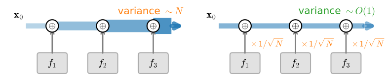
A residual network computes \(\mathbf{x}_{k+1} = \mathbf{x}_k + f_k(\mathbf{x}_k)\), so its output is the input plus the sum of \(N\) block contributions. If every block is initialized identically, each contribution has variance proportional to that of the already-inflated stream it reads, and the stream’s variance compounds geometrically with depth. This is the depth-wise cousin of the layer-wise explosion in Section 4.4. GPT-2 addresses this effect by shrinking the last linear layer of each residual branch, the output projection that writes into the stream, by a factor of \(1/\sqrt{N}\): with \(N\) roughly independent contributions each scaled down that way, the sum’s variance stays \(O(1)\) regardless of depth (Radford et al. 2019). For an \(L\)-layer transformer the published recipe is a normal with std \(0.02/\sqrt{2L}\) on the residual projections — the number of contributions is \(N = 2L\), because each layer writes to the stream twice, once from attention and once from the MLP. Unlike Xavier or He, the base 0.02 is not derived from fan-in; it is an empirical constant that worked at GPT-2’s widths and stuck.
Figure 5.3.1 draws the two regimes side by side.
5.3.3.3 Starting a Block at Zero
Zero-initializing every weight is fatal: all units in a layer compute the same output, receive the same gradient, and stay identical forever (Section 4.4). Zero-initializing just the last layer of a residual block is a different and useful move. The branch then contributes exactly nothing, each block is the identity map, and the network starts as a shallow function whose depth switches on gradually during training. Symmetry is not a problem because the branch’s earlier layers keep their random weights. On the first backward pass, the zeroed projection receives a nonzero gradient because its input is nonzero, while the earlier layers receive zero gradient through that projection. After the projection moves off zero, gradient reaches the whole branch. Keep this scheme distinct from the previous one: GPT-2 makes every residual projection small but nonzero, whereas zero-init makes one layer exactly zero so the block starts as an exact identity.
5.3.3.4 Measuring Variance across Depth
The following experiment measures variance across depth. We reuse a compact residual block (it repeats the one from Section 5.1) and stack it \(N\) deep:
class ResidualBlock(nn.Module):
    def __init__(self, d):
        super().__init__()
        self.body = nn.Sequential(nn.Linear(d, 4 * d), nn.ReLU(),
                                  nn.Linear(4 * d, d))

    def forward(self, X):
        return X + self.body(X)
class ResidualBlock(tf.keras.Model):
def __init__(self, d, out_init='he_normal'):
super().__init__()
self.body = tf.keras.Sequential([
tf.keras.layers.Dense(4 * d, kernel_initializer='he_normal'),
tf.keras.layers.ReLU(),
tf.keras.layers.Dense(d, kernel_initializer=out_init)])
def call(self, X):
return X + self.body(X)he = nnx.initializers.variance_scaling(2.0, 'fan_in', 'truncated_normal')
class ResidualBlock(nnx.Module):
def __init__(self, d, out_init=he, rngs=None):
rngs = nnx.Rngs(0) if rngs is None else rngs
self.fc1 = nnx.Linear(d, 4 * d, kernel_init=he, rngs=rngs)
self.fc2 = nnx.Linear(4 * d, d, kernel_init=out_init, rngs=rngs)
def __call__(self, X):
return X + self.fc2(nnx.relu(self.fc1(X)))he = init.MSRAPrelu(factor_type='in', slope=0.0)
class ResidualBlock(nn.Block):
def __init__(self, d, out_init=he):
super().__init__()
self.body = nn.Sequential()
self.body.add(nn.Dense(4 * d, activation='relu',
weight_initializer=he))
self.body.add(nn.Dense(d, weight_initializer=out_init))
def forward(self, X):
return X + self.body(X)Every linear layer gets He initialization, appropriate for the ReLU inside the branch. Then a named_parameters loop, the same shape as nanoGPT’s initialization code, singles out each block’s output projection and applies one of three treatments: leave it alone, scale it by \(1/\sqrt{N}\), or zero it.
Every dense layer gets He initialization, appropriate for the ReLU inside the branch; the string 'he_normal' names the same object as tf.keras.initializers.HeNormal(). The treatment is a constructor argument as well: the block takes its output projection’s initializer as a parameter, so each of the three treatments is just a different initializer. Leaving it alone means He again and zeroing is 'zeros', but scaling by \(1/\sqrt{N}\) has no menu entry, so we subclass Initializer: the instance stores the depth, and its __call__ shrinks a fresh He draw, behind the same shape-and-dtype signature everything on the menu implements.
Every dense layer gets He initialization, appropriate for the ReLU inside the branch; variance_scaling(2.0, 'fan_in', 'truncated_normal') is exactly what nnx.initializers.he_normal() expands to. The block takes its output projection’s initializer as a constructor argument, so each treatment is a different initializer. Leaving it alone means He again, scaling by \(1/\sqrt{N}\) is a closure over the depth that wraps the same three-argument signature, and zeroing is nnx.initializers.zeros.
Every dense layer gets He initialization through its weight_initializer constructor argument, which sets the per-parameter initializer that net.initialize() respects. The menu entry is init.MSRAPrelu, named after the He et al. paper’s lab: with factor_type='in' and slope=0.0 (the PReLU slope, zero for a plain ReLU) it draws a Gaussian with variance \(2/n_\textrm{in}\), exactly He normal. The treatment is a constructor argument as well: the block takes its output projection’s initializer, so each of the three treatments is just a different initializer. Leaving it alone means He again and zeroing is init.Zero(), but scaling by \(1/\sqrt{N}\) has no menu entry, so once more we subclass Initializer: the instance stores the depth, and its _init_weight shrinks a fresh He draw in place.
def init_he(module):
    if isinstance(module, nn.Linear):
        nn.init.kaiming_normal_(module.weight, nonlinearity='relu')
        nn.init.zeros_(module.bias)

def output_std(num_blocks, tweak):
    torch.manual_seed(0)
    net = nn.Sequential(*[ResidualBlock(64) for _ in range(num_blocks)])
    net.apply(init_he)
    for name, param in net.named_parameters():
        if name.endswith('body.2.weight'):  # each block's output projection
            tweak(param, num_blocks)
    torch.manual_seed(1)
    with torch.no_grad():
        return net(torch.randn(256, 64)).std().item()
class ScaledHe(tf.keras.initializers.Initializer):
def __init__(self, num_blocks):
self.num_blocks = num_blocks
def __call__(self, shape, dtype=None):
w = tf.keras.initializers.HeNormal()(shape, dtype)
return w * self.num_blocks ** -0.5
def output_std(num_blocks, out_init):
tf.keras.utils.set_random_seed(0)
net = tf.keras.Sequential(
[ResidualBlock(64, out_init=out_init(num_blocks))
for _ in range(num_blocks)])
X = tf.random.normal((256, 64), seed=1)
return float(tf.math.reduce_std(net(X)))def scaled_he(num_blocks):
def init(key, shape, dtype=jnp.float32):
return he(key, shape, dtype) * num_blocks ** -0.5
return init
def output_std(num_blocks, out_init):
rngs = nnx.Rngs(0)
net = nnx.Sequential(*[
ResidualBlock(64, out_init=out_init(num_blocks), rngs=rngs)
for _ in range(num_blocks)])
X = jax.random.normal(jax.random.key(1), (256, 64))
return net(X).std().item()class ScaledHe(init.Initializer):
def __init__(self, num_blocks):
super().__init__(num_blocks=num_blocks)
self.num_blocks = num_blocks
def _init_weight(self, name, arr):
he._init_weight(name, arr)
arr *= self.num_blocks ** -0.5
def output_std(num_blocks, out_init):
np.random.seed(0)
net = nn.Sequential()
net.add(*[ResidualBlock(64, out_init=out_init(num_blocks))
for _ in range(num_blocks)])
net.initialize() # deferred: the draws happen at the forward pass
X = np.random.normal(0, 1, (256, 64))
return float(net(X).std())One forward pass on unit-variance inputs per depth and treatment:
tweaks = {'default': lambda p, n: None,
          'scaled': lambda p, n: p.data.mul_(n ** -0.5),
          'zero': lambda p, n: nn.init.zeros_(p)}
print(f'{"N":>3}' + ''.join(f'{name:>10}' for name in tweaks))
for n in (2, 8, 32):
    stds = (output_std(n, tweak) for tweak in tweaks.values())
    print(f'{n:>3}' + ''.join(f'{s:>10.3g}' for s in stds))
N default scaled zero
2 2.81 1.91 1
8 83.5 2.38 1
32 6.37e+07 2.63 1tweaks = {'default': lambda n: 'he_normal',
'scaled': ScaledHe,
'zero': lambda n: 'zeros'}
print(f'{"N":>3}' + ''.join(f'{name:>10}' for name in tweaks))
for n in (2, 8, 32):
stds = (output_std(n, tweak) for tweak in tweaks.values())
print(f'{n:>3}' + ''.join(f'{s:>10.3g}' for s in stds)) N default scaled zero
2 3.24 1.91 1
8 99.5 2.18 1
32 7.56e+07 2.86 1tweaks = {'default': lambda n: he,
'scaled': scaled_he,
'zero': lambda n: nnx.initializers.zeros}
print(f'{"N":>3}' + ''.join(f'{name:>10}' for name in tweaks))
for n in (2, 8, 32):
stds = (output_std(n, tweak) for tweak in tweaks.values())
print(f'{n:>3}' + ''.join(f'{s:>10.3g}' for s in stds)) N default scaled zero
2 2.89 1.93 0.993
8 75.3 2.27 0.993
32 3.6e+07 2.59 0.993tweaks = {'default': lambda n: he,
'scaled': ScaledHe,
'zero': lambda n: init.Zero()}
print(f'{"N":>3}' + ''.join(f'{name:>10}' for name in tweaks))
for n in (2, 8, 32):
stds = (output_std(n, tweak) for tweak in tweaks.values())
print(f'{n:>3}' + ''.join(f'{s:>10.3g}' for s in stds)) N default scaled zero
2 2.94 1.99 0.997
8 85 2.49 0.997
32 4.75e+07 2.65 0.997The default column multiplies by a roughly constant factor per block in this unnormalized stack, reaching tens of millions by \(N=32\). Such initial activations make optimization impractical. The scaled column stays near a small constant over the depths tested: scaling cuts each branch’s variance by a factor of \(N\), following the independent-contribution approximation above. The zero column reproduces the input’s standard deviation, since every block is the identity. This forward-pass test does not prove how an optimizer will behave, but it catches an unusable initialization before training begins.
5.3.4 Custom Initializers
Some architectures require an initializer absent from the library.
In PyTorch, a custom initializer is a function that mutates a parameter.
An initializer is an object that maps (shape, dtype) to a tensor: subclass tf.keras.initializers.Initializer and implement __call__; layers then accept an instance through their initializer arguments.
In NNX, a custom initializer follows the shared (key, shape, dtype) -> array signature.
By now this is familiar: an initializer is a subclass of init.Initializer whose _init_weight method fills the array it is handed, in place, and this section has already implemented two: the truncated normal and depth-scaled He initializers.
Suppose, to make the point vividly, we want weights distributed as
\[ \begin{aligned} w \sim \begin{cases} U(5, 10) & \textrm{ with probability } \frac{1}{4} \\ 0 & \textrm{ with probability } \frac{1}{2} \\ U(-10, -5) & \textrm{ with probability } \frac{1}{4} \end{cases} \end{aligned} \]
Draw uniformly from \(U(-10, 10)\), then zero every entry of magnitude below 5:
Draw uniformly from \(U(-10, 10)\), then zero every entry of magnitude below 5. Handing an instance to kernel_initializer makes it official:
Split the key, draw a magnitude from \(U(5, 10)\), and draw a factor from \(\{-1, 0, 0, 1\}\), which zeroes the entry with probability one half and keeps either sign with probability one quarter. Handing the function to kernel_init makes it official; init gives every layer an independent key:
Draw uniformly from \(U(-10, 10)\), then zero every entry of magnitude below 5. Handing an instance to net.initialize makes it official:
def my_init(module):
    if isinstance(module, nn.Linear):
        nn.init.uniform_(module.weight, -10, 10)
        with torch.no_grad():
            module.weight *= module.weight.abs() >= 5

net.apply(my_init)
net[0].weight[:2]
tensor([[-0.0000, -0.0000, -8.7540, 0.0000],
[ 0.0000, -6.8736, 0.0000, -0.0000]], grad_fn=<SliceBackward0>)class MyInit(tf.keras.initializers.Initializer):
def __call__(self, shape, dtype=None):
w = tf.random.uniform(shape, -10, 10, dtype=dtype)
return w * tf.cast(tf.abs(w) >= 5, w.dtype)
net = tf.keras.Sequential([
tf.keras.layers.Dense(8, kernel_initializer=MyInit()),
tf.keras.layers.ReLU(),
tf.keras.layers.Dense(1)])
net(X)
net.layers[0].kernel[:2]<tf.Tensor: shape=(2, 8), dtype=float32, numpy=
array([[-0. , -5.868671, 0. , 0. , -0. , 6.156559,
-0. , 9.962585],
[ 0. , -7.492528, 0. , 0. , 0. , -0. ,
-0. , 0. ]], dtype=float32)>def my_init(key, shape, dtype=jnp.float32):
mag_key, sign_key = jax.random.split(key)
mag = jax.random.uniform(mag_key, shape, dtype, minval=5, maxval=10)
sign = jax.random.choice(sign_key, jnp.array([-1., 0., 0., 1.], dtype),
shape)
return mag * sign
net = nnx.Sequential(
nnx.Linear(4, 8, kernel_init=my_init, rngs=nnx.Rngs(0)), nnx.relu,
nnx.Linear(8, 1, rngs=nnx.Rngs(1)))
net.layers[0].kernel[:, :2]Array([[-6.4136 , 8.940486 ],
[-6.2257624, 0. ],
[ 0. , -9.485439 ],
[ 0. , 9.542628 ]], dtype=float32)class MyInit(init.Initializer):
def _init_weight(self, name, data):
data[:] = np.random.uniform(-10, 10, data.shape)
data *= np.abs(data) >= 5
net = nn.Sequential()
net.add(nn.Dense(8, activation='relu'))
net.add(nn.Dense(1))
net.initialize(MyInit())
net(X)
net[0].weight.data()[:2]array([[ 9.935757 , -0. , 0. , -7.146276 ],
[-0. , -0. , -5.6079783, -6.314646 ]])The torch.no_grad() block is required: parameters are leaf tensors that track gradients, and PyTorch rejects in-place arithmetic on them unless we declare that the mutation is not part of any computation to differentiate. (The nn.init routines run under their own no_grad internally, which is why the first line needs none.) The same context supports direct parameter edits, such as offsetting a whole matrix or assigning a single entry:
No guard is needed on the way in, because assign sits outside automatic differentiation: TensorFlow records gradients on a GradientTape, and an assignment is a write to the variable’s buffer, not an operation on the tape. The same interface supports direct parameter edits, such as offsetting a whole matrix or assigning a single entry, because slicing a variable composes with assign:
NNX parameters are mutable variables. Assignment updates the value owned by the layer while preserving the nnx.Param object that optimizers and checkpoints track. Direct parameter edits therefore use ordinary indexed assignment:
No guard is needed on the way in, because gradients are only recorded inside an autograd.record() block: outside one, indexed assignment is a plain array write. weight.data() hands back the array the parameter holds on the device, so the same interface supports direct parameter edits, such as offsetting a whole matrix or assigning a single entry:
with torch.no_grad():
    net[0].weight[:] += 1
    net[0].weight[0, 0] = 42
net[0].weight[0]
tensor([42.0000, 1.0000, -7.7540, 1.0000], grad_fn=<SelectBackward0>)w = net.layers[0].kernel
w.assign(w + 1)
w[0, 0].assign(42)
w[0]<tf.Tensor: shape=(8,), dtype=float32, numpy=
array([42. , -4.868671, 1. , 1. , 1. , 7.156559,
1. , 10.962585], dtype=float32)>net.layers[0].kernel[...] += 1
net.layers[0].kernel[0, 0] = 42
net.layers[0].kernel[0]Array([42. , 9.940486 , 1. , 1. , 1. ,
1. , -4.9630113, 1. ], dtype=float32)net[0].weight.data()[:] += 1
net[0].weight.data()[0, 0] = 42
net[0].weight.data()[0]array([42. , 1. , 1. , -6.146276])One caveat when building with lazy layers (Section 5.1.4): before the first forward pass their parameters are placeholders with no shape, so apply-based initialization and direct parameter assignment must follow the dry run that materializes them.
The ordering caveat of the lazy world (Section 5.1.4) splits by route here: a constructor initializer is stored and runs at build time, so it runs only when the variables are created. Direct assign calls require a kernel to exist and must therefore follow the first call (or an explicit build). The cells above respected that order by running net(X) before touching net.layers[0].kernel.
There is no ordering caveat: NNX parameters are created in the constructor, so both graph walks and direct assignment can run immediately.
The ordering caveat of the lazy world (Section 5.1.4) splits by route here too: initialize may run before shapes are known, since it only records which initializer to use and the draw waits for the first forward pass, but weight.data() raises a DeferredInitializationError until that pass has happened. The cells above respected the order by running net(X) before touching net[0].weight.data().
5.3.5 Summary
PyTorch initializes parameters at construction with fan-aware defaults; override them when depth, hand-made parameters, or a paper’s recipe demands it. The mechanism is one pattern: a function that dispatches on module type and mutates parameters in place with the trailing-underscore nn.init routines, walked over the model by net.apply.
Keras initializes parameters at build time, when a layer first learns its input shape, with fan-aware defaults; override them when depth or a paper’s recipe demands it. The mechanism is one pattern: an initializer is an object mapping (shape, dtype) to a tensor, handed to a layer as kernel_initializer at construction or, for a model that already exists, written into each selected kernel by a model.layers walk and assign.
NNX initializes parameters in layer constructors with fan-aware defaults; override them when depth or a paper’s recipe demands it. An initializer is a function (key, shape, dtype) -> array, handed to a layer as kernel_init at construction or run over selected modules in an existing object graph.
Gluon initializes parameters when you ask it to: initialize() records the plan, the first forward pass supplies the shapes, and the default draw, \(U(-0.07, 0.07)\), is a legacy constant rather than a fan-aware rule, so override it more readily than elsewhere. The mechanism is one pattern: an Initializer object handed to initialize on the net, a block, or a single parameter, with force_reinit=True to overwrite live values.
Beyond Xavier and He, some architectures truncate normal tails to bound outliers, scale residual output projections by \(1/\sqrt{N}\) to keep variance \(O(1)\) under the assumptions above, or zero-initialize a block’s last layer so the block initially implements the identity.
A custom scheme can be implemented with tensor operations under torch.no_grad().
A custom scheme is an Initializer subclass using tf.random code in its __call__.
A custom scheme uses jax.random behind the same three-argument signature.
A custom scheme, including truncation, is an init.Initializer subclass with a few lines of array code in its _init_weight.
5.3.6 Exercises
- [code] Layer activations across the network. Instrument the stack that
output_stdbuilds in Section 5.3.3.4 so that it records the standard deviation of the activation after every block, by running the blocks one at a time. Plot the recorded standard deviation against depth on a logarithmic axis for the default and scaled treatments at \(N=32\). - Growth per block. ● Assume that each block’s branch output is uncorrelated with the block’s input.
- Use the second-moment argument of Section 4.4.2.3 to derive the factor by which one block of the default treatment multiplies the standard deviation of the stream, and compare it with the slope of the default curve from the first exercise.
- Derive the standard deviation at the end of the scaled stack as a function of \(N\), and its limit as \(N \to \infty\).
- Zero initialization. Zero-initialize all layers of every block instead of just the output projection. The forward pass still returns the input, but what can the network learn? Work out which parameters receive a nonzero gradient, and relate the answer to the symmetry-breaking argument of Section 4.4.
- [code] Default scale. PyTorch draws both the weight and the bias of an
nn.Linearfrom \(U(-1/\sqrt{n_\textrm{in}}, 1/\sqrt{n_\textrm{in}})\).- With the biases set to zero, compute the factor by which one such layer followed by a ReLU multiplies the second moment of its input, and compare it with the factor of one that He initialization achieves (Section 4.4.2.3).
- Stack ten
nn.Linear(512, 512)layers, each followed by a ReLU, keep the default weights, zero the biases, and push unit-variance inputs through. Compare the second moment of the output, the mean of its squared entries, with your prediction. - Restore the default biases and repeat the measurement. Explain why the second moment stops shrinking after a few layers, and predict the value at which it levels off.
- [code] Default scale. Keras draws the kernel of a
Denselayer from Glorot uniform, \(U(\pm\sqrt{6/(n_\textrm{in} + n_\textrm{out})})\), and starts the bias at zero.- For a layer with \(n_\textrm{in} = n_\textrm{out}\), compute the factor by which the layer followed by a ReLU multiplies the second moment of its input, and compare it with the factor of one that He initialization achieves (Section 4.4.2.3).
- Stack ten
Dense(512)layers, each followed by a ReLU, with their default initialization, and push unit-variance inputs of width 512 through. Compare the second moment of the output, the mean of its squared entries, with your prediction.
- [code] Default scale. NNX draws the kernel of an
nnx.Linearfrom LeCun normal, a truncated normal rescaled to standard deviation \(1/\sqrt{n_\textrm{in}}\), and starts the bias at zero.- Compute the factor by which one such layer followed by a ReLU multiplies the second moment of its input, and compare it with the factor of one that He initialization achieves (Section 4.4.2.3).
- Stack ten
nnx.Linear(512, 512)layers, each followed by a ReLU, with their default initialization, and push unit-variance inputs through. Compare the second moment of the output, the mean of its squared entries, with your prediction.
- [code] Default scale. Gluon draws every
Denseweight from \(U(-0.07, 0.07)\), whatever the layer’s shape, and starts the bias at zero.- Compute, as a function of the width \(n\), the factor by which an \(n \times n\) layer followed by a ReLU multiplies the second moment of its input. At which width does it equal the factor of one that He initialization achieves (Section 4.4.2.3)?
- Stack ten
nn.Dense(n, activation='relu')layers, keep the default initialization, and push unit-variance inputs through, once for \(n = 512\) and once for \(n = 4096\). Compare the second moment of the output, the mean of its squared entries, with your predictions.
- Truncated normal. For a normal distribution truncated at \(\pm 2\sigma\): what fraction of draws does the clip discard, and by how much does it shrink the standard deviation? Neither quantity has an elementary closed form; express both in terms of the standard normal density and distribution function and evaluate them using tabulated values. Verify the standard deviation against the printed output of the demo in Section 5.3.3.1, and the discarded fraction by counting the entries of the demo’s plain normal draw that lie beyond \(\pm 2\sigma\).
- [code] Kaiming initialization. Implement the Kaiming (He) initializers of Section 4.4.2.3, uniform and normal, with an explicit
nonlinearityargument that switches the gain between'relu'and'linear'.- Check both on a \(256 \times 512\) weight by mean, standard deviation, and range: the normal initializer against the library’s He normal initializer used in Section 5.3.3.4, and the uniform initializer against its predicted bound and standard deviation. Explain any difference in range.
- Apply your normal initializer to the stack of Section 5.3.3.4, with the
'relu'gain on each block’s first layer and the'linear'gain on its output projection, and add the resulting curve to the plot of the first exercise. Does matching the per-layer gain keep the standard deviation flat across depth, and why?
- [code] Data-driven calibration. ● Initialize the stack of Section 5.3.3.4 with the default treatment, then calibrate it block by block on one mini-batch of unit-variance inputs. For each block in turn, run the mini-batch forward to that block, measure the standard deviation of its branch output \(f_k(\mathbf{x}_k)\), and rescale the block’s output projection so that this standard deviation becomes \(1/\sqrt{N}\). This adapts the layer-sequential unit-variance initialization of Mishkin and Matas (2016) to a residual stack.
- Explain why the blocks must be calibrated in order rather than all at once from a single forward pass.
- Explain why the calibration targets the branch output rather than the block output \(\mathbf{x}_k + f_k(\mathbf{x}_k)\).
- Predict the standard deviation at the end of the calibrated stack. Plot the calibrated depth-versus-standard-deviation curve next to that of the scaled treatment, and explain the difference.