%matplotlib inline
from d2l import torch as d2l
import torch
from torch.nn import functional as F10.6 What Attention Computes
Attention weights indicate how strongly each query weights each key, but do not by themselves determine the effect on the output. This section analyzes both the attention pattern and the transformed values. In an attention-only Transformer, each head factors into a QK circuit that determines attention scores and an OV circuit that transforms the attended representation. These matrices can be read directly from a checkpoint, and paths through multiple layers can be expanded algebraically. We apply this analysis to the TinyCharLM of Section 10.4 and identify a two-layer induction-head circuit on repeated random sequences (Elhage et al. 2021). The circuit is related to mechanisms observed in larger language models (Olsson et al. 2022).
%matplotlib inline
from d2l import jax as d2l
from flax import nnx
import jax
from jax import numpy as jnp
import optax
10.6.1 The Residual Stream
10.6.1.1 Residual Representations Across Layers
Write \(\mathbf{e}_{x_i} \in \mathbb{R}^d\) for the embedding of token \(x_i\) and set \(\mathbf{h}_i^{(0)} = \mathbf{e}_{x_i}\). Unrolling TinyCharLM’s forward pass, block \(\ell\) of \(L\) computes, for every position \(i\),
\[ \mathbf{h}_i^{(\ell)} = \mathbf{h}_i^{(\ell-1)} + \sum_{h=1}^{H} \sum_{j \leq i} \alpha_{ij}^{\ell h}\, \mathbf{W}_{\mathrm{OV}}^{\ell h}\, \mathbf{h}_j^{(\ell-1)}, \tag{10.6.1}\]
and the tied output head scores the final vector against every embedding, \(\mathbf{z}_i = \mathbf{E}\, \mathbf{h}_i^{(L)}\). The sequence of vectors \(\mathbf{h}_i^{(0)}, \ldots, \mathbf{h}_i^{(L)}\) is the residual stream of position \(i\). It begins with the token embedding and ends with the vector read by the output head (Figure 10.6.1). Each layer adds to this vector rather than replacing it. An attention head reads the residual streams at earlier positions, applies a linear transformation, and adds the result to the stream at the current position. Consequently, information written by one layer remains available to every later layer and to the output head.
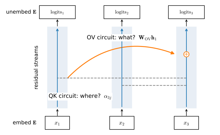
Once the attention patterns \(\alpha\) are fixed, the map from embeddings to logits in Equation 10.6.1 is linear: expanding the recursion writes it as a sum of matrix products along paths through the network. This decomposition supplies testable hypotheses about how an attention-only model computes; it does not make the learned circuit self-evident. The exact framework of Elhage et al. (2021) assumes attention-only transformers without feed-forward layers or normalization. We use the same restriction in TinyCharLM, then compare weight-level hypotheses with behavioral and intervention evidence. Real transformers contain additional nonlinear components, so the conclusions below do not transfer without new tests.
10.6.1.2 QK and OV Circuits
Each head’s term in Equation 10.6.1 splits into two independent pieces. The attention weights come from softmax over scores that depend on the query and key projections only through their product, and the payload depends only on the value and output projections:
\[ s_{ij} = \frac{\mathbf{h}_i^\top \mathbf{W}_{\mathrm{QK}}\, \mathbf{h}_j}{\sqrt{d_h}}, \qquad \mathbf{W}_{\mathrm{QK}} = \mathbf{W}_q^\top \mathbf{W}_k, \qquad \mathbf{W}_{\mathrm{OV}} = \mathbf{W}_o \mathbf{W}_v. \tag{10.6.2}\]
These equations use column vectors: \(\mathbf{W}_q\) and \(\mathbf{W}_v\) map from the residual stream into a head, while \(\mathbf{W}_o\) maps back. The code below forms the same bilinear and input–output maps in each framework’s native weight orientation; PyTorch stores linear weights transposed relative to JAX.
The QK circuit \(\mathbf{W}_{\mathrm{QK}} \in \mathbb{R}^{d \times d}\) is a bilinear form on the stream that determines the attention scores. The OV circuit \(\mathbf{W}_{\mathrm{OV}} \in \mathbb{R}^{d \times d}\) determines how an attended representation contributes to the destination. This factorization matters because the individual projections \(\mathbf{W}_q, \mathbf{W}_k, \mathbf{W}_v, \mathbf{W}_o\) are not identifiable (replacing \(\mathbf{W}_q\) by \(\mathbf{R}\mathbf{W}_q\) and \(\mathbf{W}_k\) by \(\mathbf{R}^{-\top}\mathbf{W}_k\) changes nothing the model computes), while the two products are the head itself. Both are \(d \times d\) but of rank at most \(d_h = d/H\): a head can test and move only a \(d_h\)-dimensional slice of the stream. With \(d = 128\) and four heads, each head works through a rank-32 bottleneck. In TinyCharLM the four projections live in two fused layers: qkv stacks the query, key, and value maps, and proj holds the per-head output maps side by side. Neither layer carries a bias, so the circuits of each head can be obtained by slicing these two matrices:
torch.manual_seed(0)
model = d2l.TinyCharLM(vocab_size=64, pos='rope')
D = model.token_emb.weight.shape[1]
d_h = D // model.num_heads
W = model.blks[0]['qkv'].weight        # Rows stack W_q, W_k, W_v
W_q, W_k, W_v = W[:D], W[D:2 * D], W[2 * D:]
W_o = model.blks[0]['proj'].weight     # Columns split by head
h = 0
W_QK = W_q[h * d_h:(h + 1) * d_h].T @ W_k[h * d_h:(h + 1) * d_h]
W_OV = W_o[:, h * d_h:(h + 1) * d_h] @ W_v[h * d_h:(h + 1) * d_h]
for name, M in (('W_QK', W_QK), ('W_OV', W_OV)):
    print(f'{name}: shape {tuple(M.shape)}, '
          f'rank {torch.linalg.matrix_rank(M).item()}')
W_QK: shape (128, 128), rank 32
W_OV: shape (128, 128), rank 32model = d2l.TinyCharLM(vocab_size=64, pos='rope', rngs=nnx.Rngs(0))
D = model.token_emb.embedding[...].shape[1]
d_h = D // model.num_heads
W = model.blks[0]['qkv'].kernel[...] # Columns stack W_q, W_k, W_v
W_q, W_k, W_v = W[:, :D], W[:, D:2 * D], W[:, 2 * D:]
W_o = model.blks[0]['proj'].kernel[...] # Rows split by head
h = 0
W_QK = W_q[:, h * d_h:(h + 1) * d_h] @ W_k[:, h * d_h:(h + 1) * d_h].T
W_OV = W_v[:, h * d_h:(h + 1) * d_h] @ W_o[h * d_h:(h + 1) * d_h]
for name, M in (('W_QK', W_QK), ('W_OV', W_OV)):
print(f'{name}: shape {tuple(M.shape)}, '
f'rank {jnp.linalg.matrix_rank(M)}')W_QK: shape (128, 128), rank 32
W_OV: shape (128, 128), rank 32RoPE introduces positional information into the QK circuit by rotating queries and keys before their inner product. Thus \(s_{ij}\) contains the relative rotation \(\mathbf{R}_{j-i}\) from Equation 10.4.4, whereas the values remain unrotated. Position can therefore affect the attention scores without directly changing the value transformation. We use pos='rope' below because it is the principal method studied in Section 10.4 and is used by the later models in this chapter.
10.6.1.3 Bigrams, Skip-Trigrams, and the Limits of One Layer
The path expansion shows how the class of representable functions changes with depth. With zero blocks, \(\mathbf{z}_i = \mathbf{E}\,\mathbf{e}_{x_i}\): the logits are a function of the current token only. This gives a constrained bigram model. Because the output head is tied to the embedding, the logit of token \(b\) after token \(a\) is \(\mathbf{e}_b^\top \mathbf{e}_a\), the Gram matrix of the embeddings: symmetric and of rank at most \(d\), not an arbitrary \(|\mathcal{V}| \times |\mathcal{V}|\) lookup table. Training on text fills it with as much of the bigram statistics as that form can hold. With one block,
\[ \mathbf{z}_i = \mathbf{E}\,\mathbf{e}_{x_i} + \sum_{h=1}^{H} \sum_{j \leq i} \alpha_{ij}^{h}\; \mathbf{E}\,\mathbf{W}_{\mathrm{OV}}^{h}\,\mathbf{e}_{x_j}. \tag{10.6.3}\]
Each new term has an if–then interpretation. If the QK circuit sends attention from the current token to an earlier token \(x_j\), the OV circuit adds \(\mathbf{E}\,\mathbf{W}_{\mathrm{OV}}\,\mathbf{e}_{x_j}\) to the logits. Statements of this shape are called skip-trigrams — “when \([\mathrm{A}]\) appears somewhere before \([\mathrm{B}]\), boost token \([\mathrm{C}]\)” — and they are all a one-layer model has beyond bigrams. A useful special case is copying: attend to earlier occurrences of the current token and boost that same token’s logit, so text that repeats a word becomes more likely to repeat it again.
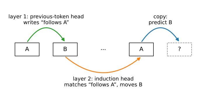
The remaining task requires composition across two layers: the sequence contains \([\mathrm{A}][\mathrm{B}] \ldots [\mathrm{A}]\), and at the second \([\mathrm{A}]\) the model should predict \([\mathrm{B}]\), continuing the pattern by finding what followed last time. No skip-trigram expresses this. The head would need to attend from the second \([\mathrm{A}]\) to the token after the earlier \([\mathrm{A}]\), but in Equation 10.6.3 the score \(\alpha_{ij}\) sees only \(\mathbf{e}_{x_i}\), \(\mathbf{e}_{x_j}\), and the offset: the key at position \(j\) contains no information about its neighbor at \(j - 1\). Content-based prediction of \([\mathrm{B}]\) requires the key to encode its predecessor. A second layer can provide this representation. A head in layer 1 attends to the previous token and writes its identity into the stream; a head in layer 2 can then match a query representing \([\mathrm{A}]\) against keys enriched with a representation of “follows \([\mathrm{A}]\)”. The head then attends to position \(j\), and its OV circuit copies \(x_j = [\mathrm{B}]\) into the destination stream (Figure 10.6.2). This two-hop circuit is the induction head: a previous-token head composing with a match-and-copy head through the residual stream. Note what the argument establishes: two layers can express it, one layer cannot, except through a position-only shortcut considered shortly. Whether gradient descent actually finds the circuit is an empirical question, and the rest of the section answers it by experiment.
10.6.2 Copying and Induction
10.6.2.1 A Repeated-Sequence Task
A controlled task can separate this mechanism from memorized corpus statistics. We train on sequences of repeated random tokens: sample a pattern of tokens uniformly from a vocabulary of 64, then tile it until the sequence is full. Within one sequence the pattern repeats; across sequences, nothing does. Every bigram is equally likely on average, so the model cannot exploit stable bigram statistics across sequences. The first pass over a pattern is unpredictable by design, while later passes are predictable from the context. The gap between first-copy and later-copy loss therefore isolates in-context retrieval more directly than an experiment on real text.
device = d2l.try_gpu()

def repeated_batch(batch_size, num_steps, vocab, Lmin, Lmax):
    """Random patterns of length Lmin..Lmax, tiled to num_steps tokens."""
    L = torch.randint(Lmin, Lmax + 1, (batch_size,), device=device)
    s = torch.randint(0, vocab, (batch_size, num_steps), device=device)
    pos = torch.arange(num_steps, device=device)
    return torch.gather(s, 1, pos[None, :] % L[:, None]), L

torch.manual_seed(0)
x, L = repeated_batch(batch_size=2, num_steps=16, vocab=10, Lmin=5, Lmax=8)
print(f'pattern lengths: {L.tolist()}')
print(x.cpu())
pattern lengths: [6, 6]
tensor([[4, 0, 3, 4, 0, 0, 4, 0, 3, 4, 0, 0, 4, 0, 3, 4],
[1, 0, 3, 5, 0, 7, 1, 0, 3, 5, 0, 7, 1, 0, 3, 5]])def repeated_batch(key, batch_size, num_steps, vocab, Lmin, Lmax):
"""Random patterns of length Lmin..Lmax, tiled to num_steps tokens."""
key_L, key_s = jax.random.split(key)
L = jax.random.randint(key_L, (batch_size,), Lmin, Lmax + 1)
s = jax.random.randint(key_s, (batch_size, num_steps), 0, vocab)
pos = jnp.arange(num_steps)
return jnp.take_along_axis(s, pos[None, :] % L[:, None], axis=1), L
x, L = repeated_batch(jax.random.key(0), batch_size=2, num_steps=16,
vocab=10, Lmin=5, Lmax=8)
print(f'pattern lengths: {L.tolist()}')
print(x)pattern lengths: [8, 6]
[[2 2 6 5 1 7 2 0 2 2 6 5 1 7 2 0]
[1 5 8 1 4 1 1 5 8 1 4 1 1 5 8 1]]The training loop is the fixed-step loop of Section 9.6 with one change: we log the loss separately on the first copy (target positions before the pattern length) and on the rest of the sequence, because the split is the measurement. Sequences are 64 tokens long and every batch is freshly sampled — the model never sees the same pattern twice.
def split_losses(logits, Y, L):
    """Cross-entropy on the first copy, on later copies, and overall."""
    ce = F.cross_entropy(logits.reshape(-1, logits.shape[-1]),
                         Y.reshape(-1), reduction='none').reshape(Y.shape)
    rep = torch.arange(1, Y.shape[1] + 1, device=device) >= L[:, None]
    return ce[~rep].mean(), ce[rep].mean(), ce.mean()

def train_repeat(model, num_steps, Lmin, Lmax, batch_size=128, vocab=64):
    model.to(device)
    optimizer = torch.optim.AdamW(model.parameters(), lr=1e-3,
                                  weight_decay=0.0)
    history = []
    for step in range(num_steps):
        x, L = repeated_batch(batch_size, 64, vocab, Lmin, Lmax)
        first, rep, loss = split_losses(model(x[:, :-1]), x[:, 1:], L)
        optimizer.zero_grad()
        loss.backward()
        optimizer.step()
        history.append((first.item(), rep.item()))
    return history

@torch.no_grad()
def eval_copy(model, Lmin, Lmax, batch_size=256, vocab=64):
    x, L = repeated_batch(batch_size, 64, vocab, Lmin, Lmax)
    logits = model(x[:, :-1])
    first, rep, _ = split_losses(logits, x[:, 1:], L)
    mask = torch.arange(1, 64, device=device) >= L[:, None]
    acc = (logits.argmax(-1) == x[:, 1:])[mask].float().mean()
    return first.item(), rep.item(), acc.item()
def split_losses(logits, Y, L):
"""Cross-entropy on the first copy, on later copies, and overall."""
ce = optax.softmax_cross_entropy_with_integer_labels(
logits.reshape(-1, logits.shape[-1]), Y.reshape(-1)).reshape(Y.shape)
rep = jnp.arange(1, Y.shape[1] + 1)[None, :] >= L[:, None]
first = (ce * ~rep).sum() / (~rep).sum()
return first, (ce * rep).sum() / rep.sum(), ce.mean()
def train_repeat(model, num_steps, Lmin, Lmax, batch_size=128, vocab=64):
optimizer = nnx.Optimizer(model, optax.adamw(1e-3, weight_decay=0.0),
wrt=nnx.Param)
@nnx.jit
def step_fn(model, optimizer, X, Y, L):
def loss_fn(model):
first, rep, loss = split_losses(model(X), Y, L)
return loss, (first, rep)
(_, (first, rep)), grads = nnx.value_and_grad(
loss_fn, has_aux=True)(model)
optimizer.update(model, grads)
return first, rep
key, history = jax.random.key(0), []
for step in range(num_steps):
key, sub = jax.random.split(key)
x, L = repeated_batch(sub, batch_size, 64, vocab, Lmin, Lmax)
first, rep = step_fn(model, optimizer, x[:, :-1], x[:, 1:], L)
history.append((float(first), float(rep)))
return history
def eval_copy(model, Lmin, Lmax, batch_size=256, vocab=64):
x, L = repeated_batch(jax.random.key(7), batch_size, 64, vocab,
Lmin, Lmax)
logits = model(x[:, :-1])
first, rep, _ = split_losses(logits, x[:, 1:], L)
mask = jnp.arange(1, 64)[None, :] >= L[:, None]
acc = ((logits.argmax(-1) == x[:, 1:]) * mask).sum() / mask.sum()
return float(first), float(rep), float(acc)10.6.2.2 A Fixed-Offset Solution
We first concatenate each length-32 pattern with itself to obtain a 64-token sequence. Although the preceding analysis rules out a one-layer content-based solution, a one-block model performs well on this fixed-period task. For this experiment alone, we enable projection biases with bias=True; their role becomes clear below.
torch.manual_seed(0)
model_shortcut = d2l.TinyCharLM(vocab_size=64, num_blks=1, pos='rope',
                                bias=True)
train_repeat(model_shortcut, 800, Lmin=32, Lmax=32)
first, rep, acc = eval_copy(model_shortcut, 32, 32)
print(f'first copy {first:.2f} nats, second copy {rep:.2f} nats, '
      f'second-copy accuracy {acc:.2f}')
first copy 4.42 nats, second copy 0.09 nats, second-copy accuracy 1.00model_shortcut = d2l.TinyCharLM(vocab_size=64, num_blks=1, pos='rope',
bias=True, rngs=nnx.Rngs(0))
train_repeat(model_shortcut, 800, Lmin=32, Lmax=32)
first, rep, acc = eval_copy(model_shortcut, 32, 32)
print(f'first copy {first:.2f} nats, second copy {rep:.2f} nats, '
f'second-copy accuracy {acc:.2f}')first copy 4.41 nats, second copy 0.09 nats, second-copy accuracy 1.00The one-block model predicts the second copy almost perfectly, but it does not implement the proposed content-based circuit. When the pattern length is always 32, the correct source for each prediction lies exactly 31 positions earlier. A RoPE head can attend to this fixed relative offset without comparing token content (Section 10.4). The following probe evaluates the same model on patterns of length 24 and measures its attention mass by relative offset:
first, rep, acc = eval_copy(model_shortcut, 24, 24)
torch.manual_seed(1)
x, L = repeated_batch(256, 64, 64, 24, 24)
m = model_shortcut.attention_weights(x[:, :-1])[0]
print(f'patterns of length 24: second-copy accuracy {acc:.2f}')
print(f'attention mass at offset 31: '
      f'{m.diagonal(-31, dim1=2, dim2=3).mean():.2f}')
print(f'attention mass at offset 23: '
      f'{m.diagonal(-23, dim1=2, dim2=3).mean():.2f}')
patterns of length 24: second-copy accuracy 0.02
attention mass at offset 31: 0.96
attention mass at offset 23: 0.00first, rep, acc = eval_copy(model_shortcut, 24, 24)
x, L = repeated_batch(jax.random.key(1), 256, 64, 64, 24, 24)
m = model_shortcut.attention_weights(x[:, :-1])[0]
print(f'patterns of length 24: second-copy accuracy {acc:.2f}')
print(f'attention mass at offset 31: '
f'{jnp.diagonal(m, -31, axis1=2, axis2=3).mean():.2f}')
print(f'attention mass at offset 23: '
f'{jnp.diagonal(m, -23, axis1=2, axis2=3).mean():.2f}')patterns of length 24: second-copy accuracy 0.02
attention mass at offset 31: 0.96
attention mass at offset 23: 0.00Accuracy falls to roughly chance because nearly all attention mass remains at offset 31 rather than moving to the offset required by the new patterns. The model has learned a fixed-offset rule rather than induction. The qkv bias facilitates this solution by providing a constant query–key pair whose RoPE-rotated score depends only on the offset, peaking at a fixed distance. With biases disabled the shortcut only half-forms (second-copy accuracy roughly 0.5–0.7 in our probe runs), which is why this demo re-enables them. Every model analyzed below keeps biases disabled, so the QK/OV algebra above remains exact. More generally, a synthetic benchmark may admit a simpler solution than the mechanism it was intended to test. We therefore sample the pattern length uniformly from 16 to 32. No fixed offset then suffices, and prediction requires content-based matching to a previous occurrence.
10.6.2.3 A Two-Block Induction Circuit
With variable pattern lengths, we train for 2,000 steps both the two-block model, the smallest model in our analysis that can express induction, and a one-block control:
torch.manual_seed(0)
model_two = d2l.TinyCharLM(vocab_size=64, num_blks=2, pos='rope')
hist_two = train_repeat(model_two, 2000, Lmin=16, Lmax=32)
torch.manual_seed(0)
model_one = d2l.TinyCharLM(vocab_size=64, num_blks=1, pos='rope')
hist_one = train_repeat(model_one, 2000, Lmin=16, Lmax=32)
for name, model in (('2 blocks', model_two), ('1 block', model_one)):
    first, rep, acc = eval_copy(model, 16, 32)
    print(f'{name}: first copy {first:.2f}, later copies {rep:.2f}, '
          f'accuracy {acc:.2f}')
2 blocks: first copy 4.50, later copies 0.45, accuracy 0.87
1 block: first copy 4.34, later copies 3.65, accuracy 0.11model_two = d2l.TinyCharLM(vocab_size=64, num_blks=2, pos='rope',
rngs=nnx.Rngs(0))
hist_two = train_repeat(model_two, 2000, Lmin=16, Lmax=32)
model_one = d2l.TinyCharLM(vocab_size=64, num_blks=1, pos='rope',
rngs=nnx.Rngs(0))
hist_one = train_repeat(model_one, 2000, Lmin=16, Lmax=32)
for name, model in (('2 blocks', model_two), ('1 block', model_one)):
first, rep, acc = eval_copy(model, 16, 32)
print(f'{name}: first copy {first:.2f}, later copies {rep:.2f}, '
f'accuracy {acc:.2f}')2 blocks: first copy 4.45, later copies 0.45, accuracy 0.87
1 block: first copy 4.31, later copies 3.67, accuracy 0.11The results support the composition argument. The two-block model reduces later-copy loss below half a nat and predicts roughly nine out of ten repeated tokens. The one-block model remains above three nats and predicts fewer than one token in five. This is better than chance because copying heads can concentrate probability on tokens present in the context, but it is substantially less accurate than retrieval. Both models remain near the chance loss of \(\ln 64\), approximately 4.2 nats, on the first copy. A slightly higher value can arise because probability assigned to repetitions is penalized when a newly sampled pattern does not repeat. The training curves also show when the performance gap develops:
def smooth(vals, k=25):
    return [sum(vals[i:i + k]) / k for i in range(0, len(vals) - k + 1, k)]

d2l.plot(list(range(0, 2000, 25)),
         [smooth([h[1] for h in hist_two]),
          smooth([h[1] for h in hist_one]),
          smooth([h[0] for h in hist_two])],
         'step', 'loss (nats)',
         legend=['later copies, 2 blocks', 'later copies, 1 block',
                 'first copy, 2 blocks'], figsize=(5, 3))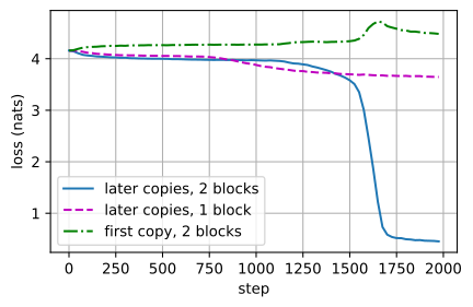
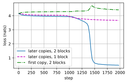
For several hundred steps, the two-block curve remains close to the one-block curve. It then falls by several nats within roughly one or two hundred steps, indicating an abrupt change in the learned computation. We observed this transition in both frameworks, although its timing varies by hundreds of steps across seeds and frameworks. A related feature appears in the training-loss derivative of larger language models and has been associated with the formation of induction heads (Olsson et al. 2022).
10.6.2.4 Inspecting the Learned Heads
TinyCharLM.attention_weights returns every head’s attention map. We feed one evaluation sequence with pattern length 24 and look at all eight heads:
torch.manual_seed(2)
x, L = repeated_batch(1, 64, 64, 24, 24)
maps = torch.stack(model_two.attention_weights(x[:, :-1]))
d2l.show_heatmaps(maps[:, 0], xlabel='key position',
                  ylabel='query position',
                  titles=[f'head {h}' for h in range(4)],
                  figsize=(9, 4.5), cmap='Blues')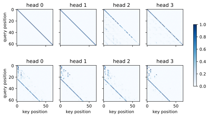
x, L = repeated_batch(jax.random.key(2), 1, 64, 64, 24, 24)
maps = jnp.stack(model_two.attention_weights(x[:, :-1]))
d2l.show_heatmaps(maps[:, 0], xlabel='key position',
                  ylabel='query position',
                  titles=[f'head {h}' for h in range(4)],
                  figsize=(9, 4.5), cmap='Blues')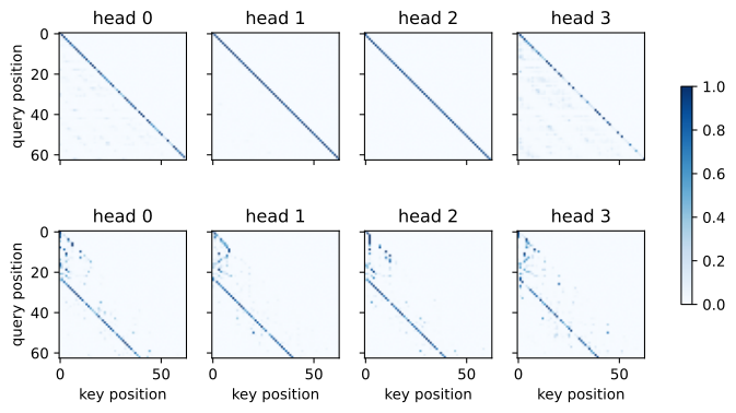
The top row is block 1, the bottom row block 2, and the two halves of the predicted circuit are both visible. In block 1, at least one head shows a sharp line one step below the diagonal — a previous-token head. In block 2, heads show a line displaced 23 steps below the diagonal, beginning where the second copy begins: attention from each query to the token after the query’s previous occurrence, which for period-24 patterns is exactly offset 23. That is the induction stripe. To quantify what the eye sees, we measure each head’s average mass on the previous token and on the induction target \(j = i + 1 - L\):
def head_scores(model, x, L):
    maps, T = model.attention_weights(x[:, :-1]), x.shape[1] - 1
    tgt = torch.arange(T, device=device)[None, :] + 1 - L[:, None]
    valid = tgt >= 0
    for b, m in enumerate(maps):
        B, H = m.shape[:2]
        prev = m.diagonal(-1, dim1=2, dim2=3).mean((0, 2))
        mass = m.gather(3, tgt.clamp(min=0)[:, None, :, None]
                        .expand(B, H, T, 1)).squeeze(-1)
        ind = (mass * valid[:, None]).sum((0, 2)) / valid.sum()
        print(f'block {b + 1}: previous token '
              + ' '.join(f'{v:.2f}' for v in prev) + ' | induction target '
              + ' '.join(f'{v:.2f}' for v in ind))

torch.manual_seed(3)
x, L = repeated_batch(256, 64, 64, 16, 32)
head_scores(model_two, x, L)
block 1: previous token 0.00 0.95 0.02 0.01 | induction target 0.00 0.00 0.01 0.00
block 2: previous token 0.04 0.05 0.04 0.04 | induction target 0.67 0.71 0.66 0.65def head_scores(model, x, L):
maps, T = model.attention_weights(x[:, :-1]), x.shape[1] - 1
tgt = jnp.arange(T)[None, :] + 1 - L[:, None]
valid = tgt >= 0
for b, m in enumerate(maps):
B, H = m.shape[:2]
prev = jnp.diagonal(m, -1, axis1=2, axis2=3).mean((0, 2))
mass = jnp.take_along_axis(
m, jnp.broadcast_to(jnp.clip(tgt, 0)[:, None, :, None],
(B, H, T, 1)), axis=3).squeeze(-1)
ind = (mass * valid[:, None]).sum((0, 2)) / valid.sum()
print(f'block {b + 1}: previous token '
+ ' '.join(f'{v:.2f}' for v in prev) + ' | induction target '
+ ' '.join(f'{v:.2f}' for v in ind))
x, L = repeated_batch(jax.random.key(3), 256, 64, 64, 16, 32)
head_scores(model_two, x, L)block 1: previous token 0.02 0.01 0.92 0.03 | induction target 0.01 0.00 0.00 0.01
block 2: previous token 0.04 0.04 0.04 0.04 | induction target 0.62 0.68 0.69 0.49In the displayed run, block 1 contains at least one head that spends well over half of its attention on the previous token and almost none on the induction target; block 2’s heads do the reverse, with the strongest putting well over half of its mass on the single position the algorithm calls for, out of up to 63 candidates. Several block-2 heads share that pattern rather than one head carrying it alone. This fixed-seed result supports the proposed two-stage mechanism, but does not estimate how reliably either the head allocation or the loss transition recurs across training runs.
10.6.3 In-Context Learning as Pattern Completion
10.6.3.1 Generalization to Unseen Patterns
Every test sequence is freshly sampled at evaluation time: the pattern it completes, and every adjacent pair inside that pattern, has never occurred in training. The parameters therefore cannot store a stable association between token pairs. Instead, the learned match-and-copy computation binds tokens to their successors at inference time within the context window. That is in-context learning, in miniature: the model “learns” each new pattern from a single exposure, without a gradient step. Plotting accuracy per position for period-24 patterns shows the single-exposure character directly:
torch.manual_seed(4)
x, L = repeated_batch(512, 64, 64, 24, 24)
with torch.no_grad():
    acc = (model_two(x[:, :-1]).argmax(-1) == x[:, 1:]).float().mean(0)
d2l.plot(torch.arange(1, 64), [acc.cpu()], 'target position', 'accuracy')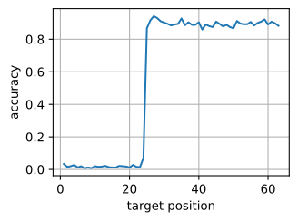
x, L = repeated_batch(jax.random.key(4), 512, 64, 64, 24, 24)
acc = (model_two(x[:, :-1]).argmax(-1) == x[:, 1:]).mean(0)
d2l.plot(jnp.arange(1, 64), [acc], 'target position', 'accuracy')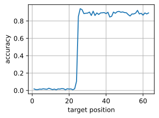
Accuracy is near zero across the whole first copy, stays low at position 24 itself — nothing in the context yet announces that repetition has begun, so the pattern’s restart is unpredictable in principle — and then jumps within a couple of positions to near-perfect for the rest of the sequence. One exposure to a pattern suffices for the model to complete the second occurrence from the preceding context. The residual imperfection has an instructive cause: when a token happens to occur twice inside one pattern with different successors, a single-token match is ambiguous, and our two-layer circuit matches on exactly one preceding token. Disambiguating would require matching on a longer prefix: deeper composition, more layers.
10.6.3.2 Verifying the Circuit in the Weights
The attention maps show where the heads attend, while the QK/OV factorization tests how they transform the attended representations directly from the weights. If block 2’s heads implement copying, then attending to token \(a\) should raise the logit of token \(a\) itself. The claim is about
\[ C_{ab} = \mathbf{e}_b^\top \mathbf{W}_{\mathrm{OV}}\, \mathbf{e}_a, \tag{10.6.4}\]
the boost that attending to token \(a\) gives to the logit of token \(b\) under a head’s OV circuit: copying means each row of the \(64 \times 64\) matrix \(\mathbf{C}\) is largest on its diagonal. We sum the OV circuits of block 2’s heads (they share the copying work) and test exactly that:
E, D = model_two.token_emb.weight, 128
qkv, proj = model_two.blks[1]['qkv'], model_two.blks[1]['proj']
OV = sum(proj.weight[:, h * 32:(h + 1) * 32]
         @ qkv.weight[2 * D + h * 32:2 * D + (h + 1) * 32]
         for h in range(4))
C = (E @ OV.T @ E.T).detach()
frac = (C.argmax(-1) == torch.arange(64, device=device)).float().mean()
print(f'rows whose largest entry is the diagonal: {frac:.2f} '
      f'(chance 1/64)')
d2l.show_heatmaps(C[None, None].cpu(), xlabel='logit boosted',
                  ylabel='token attended to', figsize=(3.6, 3.6),
                  cmap='Blues')
rows whose largest entry is the diagonal: 0.94 (chance 1/64)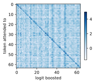
E, D = model_two.token_emb.embedding[...], 128
qkv = model_two.blks[1]['qkv'].kernel[...]
proj = model_two.blks[1]['proj'].kernel[...]
OV = sum(qkv[:, 2 * D + h * 32:2 * D + (h + 1) * 32]
         @ proj[h * 32:(h + 1) * 32] for h in range(4))
C = E @ OV @ E.T
frac = (C.argmax(-1) == jnp.arange(64)).mean()
print(f'rows whose largest entry is the diagonal: {frac:.2f} '
      f'(chance 1/64)')
d2l.show_heatmaps(C[None, None], xlabel='logit boosted',
                  ylabel='token attended to', figsize=(3.6, 3.6),
                  cmap='Blues')
rows whose largest entry is the diagonal: 0.77 (chance 1/64)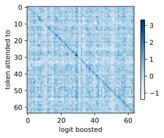
The matrix is diagonal-dominant for most tokens and for all tokens in some runs. Attending to a token therefore increases that token’s own logit more than any other logit, whereas a random argmax would match the diagonal in one row out of 64 on average. This check is deliberately partial: it feeds the OV circuit raw embeddings, ignoring what block 1 added to the stream, and it says nothing about the QK side of the match (the exercises take the analysis further, composing block 1’s OV circuit into block 2’s QK circuit). Despite this limitation, the attention pattern supplies evidence for matching and the OV matrix supplies evidence for copying. Together they support the proposed induction algorithm.
10.6.3.3 Induction Heads in Larger Models
The same type of circuit has also been observed beyond this 64-token model. Olsson et al. (2022) found induction heads in transformer language models across sizes, using a probe nearly identical to our lab: score each head by its attention from the current token to the token after that token’s previous occurrence, on repeated random sequences. Three of their observations correspond to the mechanism tested here. First, induction heads form abruptly early in training, and the formation coincides with a visible change in the loss curve, analogous to the transition measured here. Second, models gain most of their in-context learning ability in that same window, measured as the gap between loss late and early in the context; ablating induction heads after training removes a large part of that gap. Third, the heads generalize off-distribution: heads identified on repeated random tokens also complete structured patterns, translate copied text fragments, and support few-shot-like completion. Prefix matching is a general algorithm rather than a mechanism restricted to exact repetition. In larger models, feed-forward layers and normalization occur between attention operations, so the analysis is approximate and the attribution of behavior to individual components is less direct. Even so, the circuit identified in TinyCharLM provides a small, explicit model of how information introduced earlier in a context can affect later predictions.
10.6.4 What Attention Weights Do and Do Not Tell You
Attention weights are often inspected as explanations of model behavior. Their interpretation, however, requires the transformations applied to the attended representations.
An attention map specifies where a head attends but not what it computes. It fixes the mixture \(\alpha_{ij}\), but the head’s effect runs through its OV circuit: a head attending sharply to a token might move its identity, some feature of it, or, if the OV circuit annihilates the relevant directions, nothing at all. Conversely a diffuse map can implement precise computation (Section 10.3’s averaging construction did). The observation is not hypothetical: Jain and Wallace (2019) showed that on many tasks one can find quite different attention distributions that leave a model’s predictions unchanged, and the rejoinder of Wiegreffe and Pinter (2019) — that adversarially chosen alternatives do not refute every explanatory use — sharpened rather than settled the debate. “The attention weights mean something” is, as an unqualified claim, is therefore false; a useful interpretation must include the value transformation that follows the weights.
Three observations support the induction-head interpretation, with different strengths. The lower second-copy loss in the deeper model is behavioral evidence that depth enables the task, but it does not identify a component. The copying structure of an OV circuit and the associated attention pattern are weight-level evidence for a candidate mechanism, but compatible weights need not be necessary for the prediction. Changing the input period tests for a positional shortcut; only a targeted head or path ablation, followed by the predicted loss change, provides a causal intervention on the proposed circuit. Attention maps therefore locate candidates rather than establish their role.
| check in this section | evidence level | supported conclusion | remaining limitation |
|---|---|---|---|
| second-copy loss | behavioral | the deeper model fits the repeated-token task | does not identify a head |
| attention pattern | activation | a head attends with the predicted offset pattern | attention alone omits the value transformation |
| OV diagonal | weight-level | the candidate head contains a copy-compatible map | compatibility does not show necessity |
| input-period change | input intervention | separates content matching from a fixed-offset shortcut | changes the task as well as the input |
| targeted head/path ablation | component intervention | would test whether the proposed component is necessary | left as Exercise 13 rather than established here |
These checks are comparatively direct in the attention-only model because the residual update becomes linear after fixing the patterns. Feed-forward layers and normalization remove that simplification, and features in larger models may share directions. The same claims would then require separate behavioral tests, component-level interventions, and weight analysis.
10.6.5 Summary
In an attention-only transformer, each position carries a \(d\)-dimensional residual-stream vector from the embedding to the output logits. Every head factors into a QK circuit \(\mathbf{W}_q^\top \mathbf{W}_k\) that decides where to attend and an OV circuit \(\mathbf{W}_o \mathbf{W}_v\) that decides what the attended stream contributes. Both rank-\(d_h\) matrices can be read from the checkpoint. The representable functions change with depth: zero layers store bigram statistics in the low-rank Gram form the tied head allows, one layer adds skip-trigrams (including copying), and two layers can compose a previous-token head with a match-and-copy head into an induction head that finds the previous occurrence of the current token and predicts what followed it. Trained on repeated random tokens with variable period, TinyCharLM learns this circuit after an abrupt reduction in second-copy loss, while a one-block control cannot. A fixed-period version of the task is solved by a positional shortcut instead (one that a projection bias, restored for that demo alone, makes cheap to express). This comparison illustrates how synthetic benchmarks can admit unintended solutions. The trained model completes patterns it has never seen, a small instance of in-context learning, and the mechanism matches the induction heads implicated in in-context learning in large language models. Establishing this interpretation requires behavioral results, causal probes, and weight-level checks in addition to attention maps.
10.6.6 Exercises
- Tied bigrams. With zero blocks, the logit of token \(b\) after token \(a\) is \(\mathbf{e}_b^\top \mathbf{e}_a\), so the geometry of the embeddings alone fixes which successor the model prefers. Call \(b\) the top successor of \(a\) when \(\mathbf{e}_b^\top \mathbf{e}_a\) is the largest logit of that row, and assume that there are no ties.
- Show that if all embeddings have the same norm, the top successor of every token is the token itself.
- Drop the equal-norm assumption. Show that a token \(b \neq a\) can be the top successor of \(a\) only if \(\|\mathbf{e}_b\| > \|\mathbf{e}_a\|\), and conclude that the top successors cannot form a cycle \(a_1 \to a_2 \to \cdots \to a_k \to a_1\) with \(k \geq 2\).
- Suppose that in a corpus the most frequent successor of the character
tish, that ofhise, that ofeis the space, and that of the space ist. Show that no zero-block model reproduces all four as top successors, however long it is trained. - In a one-block model, every head at the first position attends only to that position. Write the logits there as \(\mathbf{E}\mathbf{M} \mathbf{e}_{x_0}\) for a matrix \(\mathbf{M}\) built from the OV circuits, and explain why neither constraint of the previous parts applies to \(\mathbf{E}\mathbf{M}\mathbf{E}^\top\).
- Head reparameterization. Replacing \(\mathbf{W}_q\) by \(\mathbf{A}\mathbf{W}_q\) and \(\mathbf{W}_k\) by \(\mathbf{A}^{-\top}\mathbf{W}_k\), for an invertible \(\mathbf{A} \in
\mathbb{R}^{d_h \times d_h}\), leaves \(\mathbf{W}_{\mathrm{QK}}\) and therefore every score of Equation 10.6.2 unchanged.
- Give the analogous substitution of \(\mathbf{W}_v\) and \(\mathbf{W}_o\) that leaves \(\mathbf{W}_{\mathrm{OV}}\) unchanged.
- The \(d \times d\) matrices of rank at most \(d_h\) form a set of dimension \(d_h(2d - d_h)\). For \(d = 128\) and \(d_h = 32\), count the parameters of one head of a
TinyCharLMwithpos='none'and the dimensions of its two circuits, and give the fraction of the parameters that the two substitutions make redundant. - Two training runs from different seeds yield layers that compute the same function. Which of \(\mathbf{W}_q\), \(\mathbf{W}_k\), \(\mathbf{W}_{\mathrm{QK}}\), \(\mathbf{W}_{\mathrm{OV}}\), and the singular values of \(\mathbf{W}_{\mathrm{OV}}\) can be compared directly between the runs? Which further symmetry of a layer with \(H\) heads must the comparison account for?
- The QK circuit under RoPE. ● With RoPE, Equation 10.4.4 turns the score of Equation 10.6.2 at offset \(\delta = j - i\) into \(\mathbf{h}_i^\top \mathbf{W}_q^\top \mathbf{R}_\delta \mathbf{W}_k
\mathbf{h}_j / \sqrt{d_h}\), where \(\mathbf{R}_\delta\) is the rotation of Equation 10.4.5 acting on the \(d_h\) coordinates of the head. Assume that \(\mathbf{W}_q\) and \(\mathbf{W}_k\) have rank \(d_h\).
- Show that the substitution \(\mathbf{W}_q \to \mathbf{A}\mathbf{W}_q\), \(\mathbf{W}_k \to \mathbf{A}^{-\top}\mathbf{W}_k\) preserves the scores at every offset if and only if \(\mathbf{A}\) commutes with every \(\mathbf{R}_\delta\).
- Let \(\mathbf{J}\) be the rotation of the plane by \(\pi/2\). A matrix that is block-diagonal with one \(2 \times 2\) block \(a_m \mathbf{I} + b_m \mathbf{J}\) per rotation pair commutes with every \(\mathbf{R}_\delta\), since each block scales and rotates its own plane. For \(d_h = 32\) the frequencies \(\omega_m\) are distinct and lie in \((0, \pi)\). Show that no other matrix commutes with every \(\mathbf{R}_\delta\), and compare the dimension of this set with the \(d_h^2\) dimensions of the substitutions available without RoPE.
- Show that an orthogonal \(\mathbf{A}\) that does not commute with \(\mathbf{R}_1\) leaves \(\mathbf{W}_{\mathrm{QK}}\) unchanged but changes the scores at nonzero offsets. Which object must a weight-level analysis of a RoPE head inspect in place of \(\mathbf{W}_{\mathrm{QK}}\)?
- Paths through two blocks. Fix the attention patterns of a model with \(L\) blocks of \(H\) heads on a sequence of \(T\) tokens, and write \(\mathbf{A}^{\ell h}\) for the \(T \times T\) matrix with entries \(\alpha_{ij}^{\ell h}\).
- Expand the logits of Equation 10.6.1 for \(L = 2\) into a sum of path terms. Show that the path through head \(h\) of block 1 and head \(h'\) of block 2 acts like a single head with pattern \(\mathbf{A}^{2h'}\mathbf{A}^{1h}\) and OV circuit \(\mathbf{W}_{\mathrm{OV}}^{2h'}\mathbf{W}_{\mathrm{OV}}^{1h}\), and bound the rank of that circuit.
- Count the path terms for \(L\) blocks, and evaluate the count for
model_two. - In a trained model the patterns of block 2 are not fixed: they depend on \(\mathbf{h}^{(1)}\) through the QK circuit of block 2. Substitute \(\mathbf{h}_i^{(1)}\) and \(\mathbf{h}_j^{(1)}\) into the score of Equation 10.6.2 and sort the terms by whether the query side, the key side, or both contain the output of a block-1 head. These terms are called Q-composition and K-composition, and the path of the first part is V-composition (Elhage et al. 2021). Which kind of term does the induction circuit of Figure 10.6.2 rely on?
- Show that two blocks can match on the two-token prefix \((x_{i-1}, x_i)\) when block 1 contains heads that attend to offsets \(-1\) and \(-2\), and name the composition term that carries each half of the match.
- [code] A copying head by hand. The skip-trigram “\([\mathrm{A}] \ldots [\mathrm{A}] \to [\mathrm{A}]\)” of Equation 10.6.3 can be built without training. Instantiate
d2l.TinyCharLM(64, num_blks=1, pos='none')and overwrite the slices of head 0 in the fusedqkvweight and inproj: set both the query and the key map to \(c\mathbf{Q}\) for a random \(d_h \times d\) matrix \(\mathbf{Q}\) and a constant \(c\), set the value map to a second random matrix \(\mathbf{V}\) and the head’s output map to \(\mathbf{V}^\top\), and zero the output maps of the other heads.- Explain why the score \(\mathbf{e}_a^\top \mathbf{W}_{\mathrm{QK}} \mathbf{e}_b\) is large exactly when \(a = b\), and why \(\mathbf{W}_{\mathrm{OV}} = \mathbf{V}^\top \mathbf{V}\) raises the logit of the attended token more than any other logit.
- Choose \(c\) so that the keys holding the query’s token receive more than \(0.9\) of the weight at every position of random 63-token sequences, and verify that the head’s contribution to the logits is largest at the current token.
- Predict the later-copy accuracy of this head on the repeated-sequence task, then measure it with
eval_copy. - With \(c = 0\) the head weights all positions \(j \leq i\) equally, so it raises the logit of each context token roughly in proportion to the token’s count. As a reference for this behavior, compute the later-copy loss and accuracy of a predictor proportional to the token counts of the context, pooled over pattern lengths uniform in 16 to 32 as
split_lossespools them. Compare both numbers witheval_copyofmodel_one, and name the information that the trained one-block RoPE model can use and this head cannot.
- [code] An offset head by hand. ● A one-block model with biases solves the fixed-period task of Section 10.6.2.2 with a head that ignores token content. Let the query and key maps of one RoPE head be zero, so that every query equals the bias \(\mathbf{b}_q \in \mathbb{R}^{d_h}\) and every key equals \(\mathbf{b}_k\). By Equation 10.4.4 the score at offset \(\delta = j - i\) is \[s(\delta) = \frac{\mathbf{b}_q^\top \mathbf{R}_\delta \mathbf{b}_k}{\sqrt{d_h}}.\]
- Show that \(\mathbf{b}_k = \mathbf{R}_{31}\mathbf{b}_q\) makes \(s(\delta)\) maximal at \(\delta = -31\), and write \(s(\delta)\) as a sum over the 16 rotation pairs of Equation 10.4.5, with the frequencies \(\omega_m = 10000^{-2m/d_h}\) that
TinyCharLMuses. - Spread \(\|\mathbf{b}_q\|^2\) equally over the pairs, and find the \(\|\mathbf{b}_q\|^2\) at which the query at position 62 places \(0.9\) of its weight on offset \(-31\).
- Repeat the last computation with all of \(\|\mathbf{b}_q\|^2\) in the fastest pair, and find the offsets that then compete with \(-31\). Find an allocation over the pairs that needs a smaller norm than equal spreading, and explain the result through the periods \(2\pi/\omega_m\) relative to the 63 offsets a query can see.
- For which pattern lengths does a head that always copies the token at offset \(-31\) predict every target at position 32 or later correctly?
- Show that \(\mathbf{b}_k = \mathbf{R}_{31}\mathbf{b}_q\) makes \(s(\delta)\) maximal at \(\delta = -31\), and write \(s(\delta)\) as a sum over the 16 rotation pairs of Equation 10.4.5, with the frequencies \(\omega_m = 10000^{-2m/d_h}\) that
- [code] The Bayes-optimal predictor. ● In the task of Section 10.6.2.3, the pattern length \(L\) is uniform on \(\{16, \ldots, 32\}\) and the pattern tokens are uniform over 64 values. The Bayes-optimal prediction of \(x_t\) from \(x_0, \ldots,
x_{t-1}\) averages the predictions of all pattern lengths \(L'\), weighted by their posterior probabilities, and no model achieves a lower expected loss.
- Show that the prefix \(x_0, \ldots, x_{t-1}\) has probability \(64^{-\min(L', t)}\) under every length \(L'\) with which it is consistent. Neglecting shorter lengths that are consistent by chance, derive the posterior weight of the true length at \(t = L\) and at \(t = L + 1\).
- At \(16 \leq t < L\) the true distribution of \(x_t\) is uniform. Show that the predictor’s distribution there is not, and conclude that its first-copy loss exceeds \(\ln 64\).
- Simulate the predictor and report its first-copy loss, later-copy loss, and later-copy accuracy, pooled over positions as
split_lossesandeval_copypool them. Compare the results withmodel_two. - Section 10.6.3.1 states that the restart at position 24 of a period-24 pattern is unpredictable in principle. Compute the probability that the Bayes-optimal predictor assigns to the correct token there, and determine whether its most probable token is correct. In which sense does the statement hold?
- [code] Positional schemes and induction. ● The induction circuit needs a previous-token head in block 1 and, in block 2, a match with a key 15 to 31 positions back.
- In a
pos='none'model, permuting \(x_0, \ldots, x_{i-1}\) leaves the output of block 1 at position \(i\) unchanged, because the causal mask treats all earlier keys alike. Conclude that no block-1 head of such a model can be a previous-token head. - The ALiBi bias of Equation 10.4.6 is largest at offset \(0\). Show that a content score with a large penalty on keys holding the query’s own token moves the peak of a block-1 ALiBi head to offset \(-1\), and compute the weight it then places on offset \(-1\) on long random sequences for each of the four slopes. Which of the four heads, if any, is a previous-token head? Then compute the penalty that each head pays in block 2 for a match at distance 15 to 31.
- The timing of the loss transition varies across seeds. Retrain the
'rope'model of Section 10.6.2.3 with three further seeds and record the step at which the smoothed later-copy loss first falls below 2 nats. - Retrain with
pos='none'and withpos='alibi', reporteval_copyandhead_scores, and compare the transition steps with the seed spread of the previous part. Which schemes develop induction heads, and which heads of the ALiBi model carry the match?
- In a
- [code] Repeated tokens within a pattern. ● Section 10.6.3.1 attributes the remaining errors of
model_twoto tokens that occur more than once in a pattern with different successors, which a match on a single token cannot tell apart.- For a pattern of \(L\) tokens drawn uniformly from 64 values, compute the probability that the token at a given position occurs elsewhere in the pattern. A circuit that picks one of the \(K\) successors of the current token uniformly, when that token occurs \(K\) times in the pattern, is correct with probability \(1/K\). Compute its expected accuracy \(\mathbb{E}[1/K]\) in closed form, and evaluate both quantities for \(L = 21\).
- Evaluate
model_twoon patterns of length 21, whichrepeated_batchtiles to three copies within 64 tokens. Split the later-copy targets by whether the current token is unique in the pattern, and report the accuracy of each group on the second and on the third copy. Compare the overall accuracy with \(\mathbb{E}[1/K]\). - Explain the results through the single-token match. What does an additional earlier occurrence with the same successor do to the attention pattern and to the output, and what does one with a different successor do?
- Two blocks can match on the two-token prefix \((x_{i-1}, x_i)\) when block 1 contains heads that attend to offsets \(-1\) and \(-2\). Measure the attention mass that each block-1 head of
model_twoplaces at offset \(-2\), and decide from this and your earlier measurements whethermodel_twomatches on more than one token.
- [code] A vocabulary split. ● Every test pattern of Section 10.6.3.1 is new, but each of its tokens has occurred as an input during training. Retrain the two-block model of Section 10.6.2.3 with
train_repeatandvocab=48, so that training patterns use only tokens 0 to 47 while the model keeps all 64 embeddings.- Report the later-copy loss and accuracy on patterns drawn from tokens 48 to 63 and, as a control with a vocabulary of the same size, on patterns drawn from tokens 0 to 15.
- The held-out tokens never appear as inputs or as targets, but through the tied output head their embeddings still receive a gradient at every training position. Find the direction in which these gradients move their embeddings.
- The copy matrix Equation 10.6.4 of a held-out token applies an OV circuit trained only on streams of tokens 0 to 47 to an embedding shaped only by its initialization and the gradients of the previous part. Compute the copy matrix restricted to the held-out tokens and restricted to tokens 0 to 15, compare their diagonal fractions, and relate the difference to the accuracies of the first part.
- [code] K-composition in the weights. ● The match of the induction head works because the QK circuit of block 2 reads what the OV circuit of block 1 wrote into the stream.
- For every pair of head \(h\) of block 1 and head \(h'\) of block 2 of
model_two, compute the \(64 \times 64\) matrix \[\mathbf{E}\, \mathbf{W}_{\mathrm{QK}}^{2h'}\, \mathbf{W}_{\mathrm{OV}}^{1h}\, \mathbf{E}^\top, \tag{10.6.5}\] whose entry \((a, b)\) scores a query token \(a\) against a key whose predecessor was \(b\). Measure the fraction of rows whose largest entry lies on the diagonal, as the copy test of Equation 10.6.4 does for copying. - Compare with the direct path \(\mathbf{E}\,
\mathbf{W}_{\mathrm{QK}}^{2h'}\, \mathbf{E}^\top\) of the same block-2 heads. Which pairs of heads carry the match, and do they agree with the attention-based scores of
head_scores? - The computation ignores the rotation that RoPE applies inside the QK circuit. Include it for a fixed offset with Equation 10.4.4, and check whether doing so at offset \(-23\) changes the ranking of the pairs.
- For every pair of head \(h\) of block 1 and head \(h'\) of block 2 of
- Weights that change nothing. The output of a head at query \(i\) is \(\mathbf{W}_{\mathrm{OV}} \sum_j \alpha_{ij}\, \mathbf{h}_j\) by Equation 10.6.1, and the softmax makes every weight \(\alpha_{ij}\) on an unmasked key positive.
- Show that the attention distributions over \(n\) keys that give the same head output as \(\boldsymbol{\alpha}_i\) contain, around \(\boldsymbol{\alpha}_i\), a piece of an affine subspace of dimension at least \(n - 1 - d_h\). Evaluate the bound for the last query of a 63-token input to
model_two. - The alternatives of the first part are constructed for one input at a time, as are those of Jain and Wallace (2019) . State the condition under which a family of alternatives can be the attention patterns of one head with other QK weights on every input at once. Explain why this condition, raised by Wiegreffe and Pinter (2019), weakens the argument that the existence of alternative distributions disqualifies attention weights as explanations.
- Show that the attention distributions over \(n\) keys that give the same head output as \(\boldsymbol{\alpha}_i\) contain, around \(\boldsymbol{\alpha}_i\), a piece of an affine subspace of dimension at least \(n - 1 - d_h\). Evaluate the bound for the last query of a 63-token input to
- [code] Circuit ablation. The last row of Table 10.6.1 leaves the component intervention to this problem.
- Explain why zeroing a head’s slice of
projremoves exactly that head’s contribution to the residual stream, and which attention patterns this intervention leaves unchanged and which it can alter. - Zero each block-2 head of
model_twoin turn and measure the later-copy loss and accuracy witheval_copy; then do the same for each block-1 head. - Ablate together the two block-2 heads with the highest induction-target scores in
head_scores. Does the sum of the two single-head loss increases predict the joint increase, and what does the comparison say about redundancy between the heads? - Which of the remaining limitations listed in Table 10.6.1 does this experiment remove, and which does it leave?
- Explain why zeroing a head’s slice of
- [extended] Induction heads in text. ● Olsson et al. (2022) tie the formation of induction heads in language models to an abrupt gain in in-context learning, measured as the drop in loss from early to late positions of the context. Test this on the character-level model of
Section 10.4.4.3.
- Train
d2l.TinyCharLMwithpos='rope'on the character-level Time Machine data of Section 10.4.4.3 in 30 rounds of 100 steps ofd2l.train_lm. After each round, record two quantities. The first is the largest induction-target score of a block-2 head on repeated random sequences over the text vocabulary with pattern lengths 16 to 32, computed with a variant ofhead_scoresthat returns its scores. The second is the in-context gain, the validation loss at target positions 0 to 15 minus that at positions 96 to 127. - Plot both quantities against the training step. Do the induction score and the in-context gain rise in the same window?
- After training, zero the block-2 heads with the highest induction scores and measure the in-context gain and the validation loss again. How much of the gain do these heads carry?
- The repeated random sequences contain no structure besides repetition, while text repeats words and phrases at irregular distances. Which of your results would change if the text contained no repeated words, and why?
- Train