import torch
from torch import nn6.3 Padding and Stride
Recall the example of a convolution in Figure 6.2.1. The input had both a height and width of 3 and the convolution kernel had both a height and width of 2, yielding an output representation with dimension \(2\times2\). Assuming that the input shape is \(n_\textrm{h}\times n_\textrm{w}\) and the convolution kernel shape is \(k_\textrm{h}\times k_\textrm{w}\), the output shape is \((n_\textrm{h}-k_\textrm{h}+1) \times (n_\textrm{w}-k_\textrm{w}+1)\) because the kernel must remain within the input.
This section introduces padding, stride, and dilation. Together they control the output size and the region of the input that contributes to each output element. Because kernels usually have width and height greater than \(1\), successive unpadded convolutions progressively reduce the spatial dimensions. If we start with a \(240 \times 240\) pixel image, ten unpadded layers of \(5 \times 5\) convolutions reduce the representation to \(200 \times 200\) pixels. The surviving outputs are centered away from the original boundary, and boundary pixels influence far fewer activations than interior pixels. Padding controls this shrinkage and increases the use of boundary pixels. When a lower-resolution representation is desired, a strided convolution performs convolution and downsampling in one operation. Dilation enlarges a kernel’s effective field of view without increasing its number of parameters.
import tensorflow as tffrom d2l import jax as d2l
from flax import nnx
import jax
from jax import numpy as jnpfrom mxnet import np, npx
from mxnet.gluon import nn
npx.set_np()6.3.1 Padding
Unpadded convolutions use boundary pixels less often than interior pixels and eventually remove them from the representation. Figure 6.3.1 shows how utilization depends on kernel size and position.
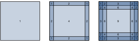
Each convolution with a small kernel removes only a few positions, but the loss accumulates across layers. We can instead add pixels around the input boundary, increasing its effective size. Typically, we set the values of the extra pixels to zero. In Figure 6.3.2, we pad a \(3 \times 3\) input, increasing its size to \(5 \times 5\). The corresponding output then increases to a \(4 \times 4\) matrix. The shaded portions are the first output element as well as the input and kernel tensor elements used for the output computation: \(0\times0+0\times1+0\times2+0\times3=0\).
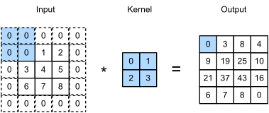
In general, if we add a total of \(p_\textrm{h}\) rows of padding (roughly half on top and half on bottom) and a total of \(p_\textrm{w}\) columns of padding (roughly half on the left and half on the right), the output shape will be
\[(n_\textrm{h}-k_\textrm{h}+p_\textrm{h}+1)\times(n_\textrm{w}-k_\textrm{w}+p_\textrm{w}+1). \tag{6.3.1}\]
This means that the height and width of the output will increase by \(p_\textrm{h}\) and \(p_\textrm{w}\), respectively.
In many cases, we will want to set \(p_\textrm{h}=k_\textrm{h}-1\) and \(p_\textrm{w}=k_\textrm{w}-1\) to give the input and output the same height and width. This choice makes the output shape of each layer predictable. Assuming that \(k_\textrm{h}\) is odd here, we will pad \(p_\textrm{h}/2\) rows on both sides of the height. If \(k_\textrm{h}\) is even, one possibility is to pad \(\lceil p_\textrm{h}/2\rceil\) rows on the top of the input and \(\lfloor p_\textrm{h}/2\rfloor\) rows on the bottom. We will pad both sides of the width in the same way.
CNNs commonly use convolution kernels with odd height and width values, such as 1, 3, 5, or 7. Choosing odd kernel sizes has the benefit that we can preserve the dimensionality while padding with the same number of rows on top and bottom, and the same number of columns on left and right.
Odd kernels with shape-preserving padding also provide a convenient alignment. Take any two-dimensional tensor X, an odd kernel size, and the same number of padding rows and columns on all sides, so that the output has the same height and width as the input. The output Y[i, j] is then calculated by cross-correlation of the input and convolution kernel with the window centered on X[i, j].
In the following example, we create a two-dimensional convolutional layer with a height and width of 3 and apply 1 pixel of padding on all sides. Given an input with a height and width of 8, we find that the height and width of the output is also 8.
# We define a helper function to calculate convolutions. It initializes the
# convolutional layer weights and performs corresponding dimensionality
# elevations and reductions on the input and output
def comp_conv2d(conv2d, X):
    # (1, 1) indicates that batch size and the number of channels are both 1
    X = X.reshape((1, 1) + X.shape)
    Y = conv2d(X)
    # Strip the first two dimensions: examples and channels
    return Y.reshape(Y.shape[2:])

# 1 row and column is padded on either side, so a total of 2 rows or columns
# are added
conv2d = nn.LazyConv2d(1, kernel_size=3, padding=1)
X = torch.rand(size=(8, 8))
comp_conv2d(conv2d, X).shape
torch.Size([8, 8])# We define a helper function to calculate convolutions. It initializes
# the convolutional layer weights and performs corresponding dimensionality
# elevations and reductions on the input and output
def comp_conv2d(conv2d, X):
# (1, 1) indicates that batch size and the number of channels are both 1
X = tf.reshape(X, (1, ) + X.shape + (1, ))
Y = conv2d(X)
# Strip the first two dimensions: examples and channels
return tf.reshape(Y, Y.shape[1:3])
# 1 row and column is padded on either side, so a total of 2 rows or columns
# are added
conv2d = tf.keras.layers.Conv2D(1, kernel_size=3, padding='same')
X = tf.random.uniform(shape=(8, 8))
comp_conv2d(conv2d, X).shapeTensorShape([8, 8])# We define a helper function to calculate convolutions. It initializes
# the convolutional layer weights and performs corresponding dimensionality
# elevations and reductions on the input and output
def comp_conv2d(conv2d, X):
# (1, X.shape, 1) indicates that batch size and the number of channels are both 1
X = X.reshape((1,) + X.shape + (1,))
Y = conv2d(X)
# Strip the dimensions: examples and channels
return Y.reshape(Y.shape[1:3])
# 1 row and column is padded on either side, so a total of 2 rows or columns are added
conv2d = nnx.Conv(1, 1, kernel_size=(3, 3), padding='SAME',
rngs=nnx.Rngs(d2l.get_key()))
X = jax.random.uniform(d2l.get_key(), shape=(8, 8))
comp_conv2d(conv2d, X).shape(8, 8)# We define a helper function to calculate convolutions. It initializes
# the convolutional layer weights and performs corresponding dimensionality
# elevations and reductions on the input and output
def comp_conv2d(conv2d, X):
conv2d.initialize()
# (1, 1) indicates that batch size and the number of channels are both 1
X = X.reshape((1, 1) + X.shape)
Y = conv2d(X)
# Strip the first two dimensions: examples and channels
return Y.reshape(Y.shape[2:])
# 1 row and column is padded on either side, so a total of 2 rows or columns are added
conv2d = nn.Conv2D(1, kernel_size=3, padding=1)
X = np.random.uniform(size=(8, 8))
comp_conv2d(conv2d, X).shape(8, 8)When the height and width of the convolution kernel are different, we can make the output and input have the same height and width by setting different padding numbers for height and width.
# We use a convolution kernel with height 5 and width 3. The padding on either
# side of the height and width are 2 and 1, respectively
conv2d = nn.LazyConv2d(1, kernel_size=(5, 3), padding=(2, 1))
comp_conv2d(conv2d, X).shape
torch.Size([8, 8])# We use a convolution kernel with height 5 and width 3. The padding on
# either side of the height and width are 2 and 1, respectively
conv2d = tf.keras.layers.Conv2D(1, kernel_size=(5, 3), padding='same')
comp_conv2d(conv2d, X).shapeTensorShape([8, 8])# We use a convolution kernel with height 5 and width 3. The padding on
# either side of the height and width are 2 and 1, respectively
conv2d = nnx.Conv(1, 1, kernel_size=(5, 3), padding=(2, 1),
rngs=nnx.Rngs(d2l.get_key()))
comp_conv2d(conv2d, X).shape(8, 8)# We use a convolution kernel with height 5 and width 3. The padding on
# either side of the height and width are 2 and 1, respectively
conv2d = nn.Conv2D(1, kernel_size=(5, 3), padding=(2, 1))
comp_conv2d(conv2d, X).shape(8, 8)6.3.2 Stride
When computing the cross-correlation, we start with the convolution window at the upper-left corner of the input tensor, and then slide it over all locations both down and to the right. In the previous examples, we defaulted to sliding one element at a time. For computational efficiency or downsampling, we can move the window by more than one element and skip intermediate positions. This can be useful when a large kernel already covers a broad input region.
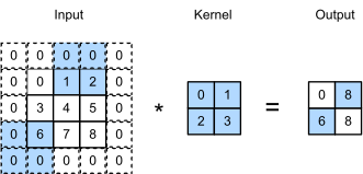
We refer to the number of rows and columns traversed per slide as stride. So far, we have used strides of 1, both for height and width. Sometimes, we may want to use a larger stride. Figure 6.3.3 shows a two-dimensional cross-correlation operation with a stride of 3 vertically and 2 horizontally. The shaded portions are the output elements as well as the input and kernel tensor elements used for the output computation: \(0\times0+0\times1+1\times2+2\times3=8\), \(0\times0+6\times1+0\times2+0\times3=6\). We can see that when the second element of the first column is generated, the convolution window slides down three rows. The convolution window slides two columns to the right when the second element of the first row is generated. When the convolution window continues to slide two columns to the right on the input, there is no output because the input element cannot fill the window (unless we add another column of padding).
In general, when the stride for the height is \(s_\textrm{h}\) and the stride for the width is \(s_\textrm{w}\), the output shape is
\[\lfloor(n_\textrm{h}-k_\textrm{h}+p_\textrm{h}+s_\textrm{h})/s_\textrm{h}\rfloor \times \lfloor(n_\textrm{w}-k_\textrm{w}+p_\textrm{w}+s_\textrm{w})/s_\textrm{w}\rfloor. \tag{6.3.2}\]
If we set \(p_\textrm{h}=k_\textrm{h}-1\) and \(p_\textrm{w}=k_\textrm{w}-1\), then the output shape can be simplified to \(\lfloor(n_\textrm{h}+s_\textrm{h}-1)/s_\textrm{h}\rfloor \times \lfloor(n_\textrm{w}+s_\textrm{w}-1)/s_\textrm{w}\rfloor\). Going a step further, if the input height and width are divisible by the strides on the height and width, then the output shape will be \((n_\textrm{h}/s_\textrm{h}) \times (n_\textrm{w}/s_\textrm{w})\).
Below, we set the strides on both the height and width to 2, thus halving the input height and width.
conv2d = nn.LazyConv2d(1, kernel_size=3, padding=1, stride=2)
comp_conv2d(conv2d, X).shape
torch.Size([4, 4])conv2d = tf.keras.layers.Conv2D(1, kernel_size=3, padding='same', strides=2)
comp_conv2d(conv2d, X).shapeTensorShape([4, 4])conv2d = nnx.Conv(1, 1, kernel_size=(3, 3), padding=1, strides=2,
rngs=nnx.Rngs(d2l.get_key()))
comp_conv2d(conv2d, X).shape(4, 4)conv2d = nn.Conv2D(1, kernel_size=3, padding=1, strides=2)
comp_conv2d(conv2d, X).shape(4, 4)The following example uses different settings along the two axes.
conv2d = nn.LazyConv2d(1, kernel_size=(3, 5), padding=(0, 1), stride=(3, 4))
comp_conv2d(conv2d, X).shape
torch.Size([2, 2])# tf.keras.Conv2D accepts only 'same'/'valid' for `padding`; we use a
# ZeroPadding2D layer to apply padding=(0, 1) (matching the MX/PT/JAX
# tabs) before the convolution.
conv2d = tf.keras.Sequential([
tf.keras.layers.ZeroPadding2D(padding=(0, 1)),
tf.keras.layers.Conv2D(1, kernel_size=(3, 5), padding='valid',
strides=(3, 4))])
comp_conv2d(conv2d, X).shapeTensorShape([2, 2])conv2d = nnx.Conv(1, 1, kernel_size=(3, 5), padding=(0, 1), strides=(3, 4),
rngs=nnx.Rngs(d2l.get_key()))
comp_conv2d(conv2d, X).shape(2, 2)conv2d = nn.Conv2D(1, kernel_size=(3, 5), padding=(0, 1), strides=(3, 4))
comp_conv2d(conv2d, X).shape(2, 2)6.3.3 Dilation
Padding and stride change where the kernel is applied. A third modification changes the kernel’s footprint itself: a dilated convolution (Yu and Koltun 2016) places the kernel taps \(d\) pixels apart instead of at adjacent positions, where \(d\) is called the dilation (or dilation rate). A \(k_\textrm{h} \times k_\textrm{w}\) kernel with dilation \(d\) still has \(k_\textrm{h} k_\textrm{w}\) weights, but along each axis the taps now span a window of
\[k' = k + (k-1)(d-1) = d(k-1)+1 \tag{6.3.3}\]
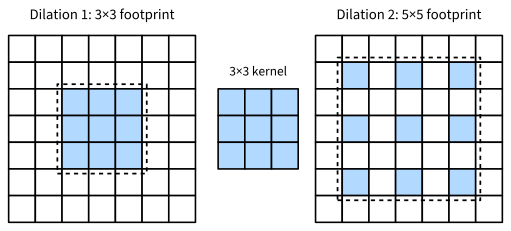
pixels, the effective kernel size. Setting \(d=1\) recovers the ordinary convolution. Figure 6.3.4 shows a \(3 \times 3\) kernel at dilations 1 and 2: at dilation 2 the nine taps spread over a \(5 \times 5\) footprint, skipping every other pixel, while the cost of applying the kernel is unchanged.
For output shapes, a dilated kernel behaves exactly like a dense kernel of its effective size. Substituting \(k'\) into the strided formula above gives the general form covering padding, stride, and dilation at once:
\[\lfloor(n_\textrm{h}-d_\textrm{h}(k_\textrm{h}-1)+p_\textrm{h}+s_\textrm{h}-1)/s_\textrm{h}\rfloor \times \lfloor(n_\textrm{w}-d_\textrm{w}(k_\textrm{w}-1)+p_\textrm{w}+s_\textrm{w}-1)/s_\textrm{w}\rfloor. \tag{6.3.4}\]
With \(d_\textrm{h}=d_\textrm{w}=1\) this reduces to the strided formula, and with unit stride and no padding to the \((n-k+1)\) rule we started from.
Dilation enlarges the receptive field without adding kernel parameters. In the receptive-field formula Equation 6.2.3, each layer contributes \(k'_i - 1 = d_i(k_i - 1)\) at stride 1, so doubling the dilation at every layer, \(d_i = 1, 2, 4, \ldots, 2^{L-1}\) for \(3 \times 3\) kernels, yields a receptive field of side \(2^{L+1}-1\): it grows exponentially with depth while every layer costs the same nine multiplications per output. The alternative route to a large receptive field, striding, pays for it by shrinking the output. This makes dilation the standard tool for dense prediction tasks such as semantic segmentation, where every pixel needs wide context but the output must keep the input’s resolution; we will meet it again in the fully convolutional networks of Section 20.11.
We verify the effective-size calculation numerically: on our \(8 \times 8\) input, a \(3 \times 3\) kernel at dilation 2 produces the same \(4 \times 4\) output as a dense \(5 \times 5\) kernel.
# Dilation 2 gives the 3x3 kernel a 5x5 footprint, so both convolutions
# shrink the 8x8 input to 4x4
conv2d = nn.LazyConv2d(1, kernel_size=3, dilation=2)
conv5 = nn.LazyConv2d(1, kernel_size=5)
comp_conv2d(conv2d, X).shape, comp_conv2d(conv5, X).shape
(torch.Size([4, 4]), torch.Size([4, 4]))# Dilation 2 gives the 3x3 kernel a 5x5 footprint, so both convolutions
# shrink the 8x8 input to 4x4
conv2d = tf.keras.layers.Conv2D(1, kernel_size=3, padding='valid',
dilation_rate=2)
conv5 = tf.keras.layers.Conv2D(1, kernel_size=5, padding='valid')
comp_conv2d(conv2d, X).shape, comp_conv2d(conv5, X).shape(TensorShape([4, 4]), TensorShape([4, 4]))# Dilation 2 gives the 3x3 kernel a 5x5 footprint, so both convolutions
# shrink the 8x8 input to 4x4
conv2d = nnx.Conv(1, 1, kernel_size=(3, 3), padding='VALID',
kernel_dilation=2, rngs=nnx.Rngs(d2l.get_key()))
conv5 = nnx.Conv(1, 1, kernel_size=(5, 5), padding='VALID',
rngs=nnx.Rngs(d2l.get_key()))
comp_conv2d(conv2d, X).shape, comp_conv2d(conv5, X).shape((4, 4), (4, 4))# Dilation 2 gives the 3x3 kernel a 5x5 footprint, so both convolutions
# shrink the 8x8 input to 4x4
conv2d = nn.Conv2D(1, kernel_size=3, dilation=2)
conv5 = nn.Conv2D(1, kernel_size=5)
comp_conv2d(conv2d, X).shape, comp_conv2d(conv5, X).shape((4, 4), (4, 4))6.3.4 Summary and Discussion
Padding can increase the height and width of the output and is often chosen so that input and output have the same spatial shape. It lets boundary pixels affect outputs centered near the boundary, but does not make their use identical to that of interior pixels: a corner pixel still belongs to fewer windows containing real image values. Typically we pick symmetric padding on both sides of the input height and width. In this case we refer to \((p_\textrm{h}, p_\textrm{w})\) padding. Most commonly we set \(p_\textrm{h} = p_\textrm{w}\), in which case we say that we choose padding \(p\).
A similar convention applies to strides. When the vertical stride \(s_\textrm{h}\) and horizontal stride \(s_\textrm{w}\) match, we refer to stride \(s\). A stride of \(n > 1\) can reduce each output dimension to \(1/n\) of the corresponding input dimension. The same shorthand covers dilation: when \(d_\textrm{h} = d_\textrm{w}\), we speak of dilation \(d\). Dilation widens the region seen by each output without adding weights or reducing resolution, as required for dense prediction. By default, padding is 0 and stride and dilation are 1.
The examples above use zero padding. Libraries can implement it without allocating a larger tensor, but it imposes a boundary condition: values outside the image are treated as zero. Filters that overlap the border therefore receive systematically different inputs from interior filters, and the artifacts can propagate through the feature maps (Alsallakh et al. 2020). Padding also conveys absolute position because a unit can infer its proximity to a border from the zeros it sees. Reflect padding mirrors border rows and columns, while replicate padding repeats them; these alternatives can reduce visible border artifacts, for example in image generation.
6.3.5 Exercises
[code] Output shapes.
- For the last example of Section 6.3.2, with kernel size \((3, 5)\), padding \((0, 1)\), and stride \((3, 4)\) on the \(8 \times 8\) input, calculate the output shape by hand and check that it is consistent with the experimental result.
- Using Equation 6.3.4, predict the output shape for a \(7 \times 7\) kernel with dilation \((3, 3)\), stride \((3, 3)\), and no padding on a \(32 \times 32\) input. Verify the prediction with
comp_conv2din two steps: apply the dilated kernel at stride 1, then keep every third row and column of the result.
Adapted from Simon Prince, Understanding Deep Learning, Problems 10.2 and 10.4.
[code] Mirror padding. Mirror padding, also called reflect padding, extends a tensor by reflecting its entries about the border without repeating the border entry: padding the vector \((1, 2, 3)\) by one entry on each side gives \((2, 1, 2, 3, 2)\).
- Implement mirror padding by one entry on every side of a two-dimensional tensor, and check the result by hand on a \(3 \times 3\) tensor with distinct entries.
- Pad a \(5 \times 5\) tensor of ones by one entry on every side, once with zeros and once with mirror padding. Apply
corr2dfrom Section 6.2 to each padded tensor with a \(3 \times 3\) kernel whose entries all equal \(\frac{1}{9}\). Compare the two outputs at the corners, along the edges, and in the interior, and relate the difference to the boundary condition that zero padding imposes.
Benefits of stride. A \(3 \times 3\) convolution with one pixel of padding on every side is applied to a single-channel \(64 \times 64\) input.
- Count the multiplications this layer performs at stride 1 and at stride 2. By what factor does stride 2 reduce the cost of a second, stride-1 layer of the same kind placed after this one?
- Four such layers are stacked. Use Equation 6.2.3 to compute the receptive field of one output element when all four layers have stride 1 and when the first two have stride 2. Use the comparison to give one statistical benefit of a stride larger than 1.
Fractional stride. ● Read a stride of \(\frac{1}{2}\) as moving the convolution window by half an input element per output element.
- Evaluate Equation 6.3.4 at \(d_\textrm{h} = 1\), \(s_\textrm{h} = \frac{1}{2}\), and \(p_\textrm{h} = k_\textrm{h} - 1\). How does the output height compare with the input height?
- Describe how to compute this output with an ordinary stride-1 convolution applied to a modified input, and check that your construction gives the same output height.
- Name a task in which a network needs this operation, and say where in the network it would be placed.
Stride as sampling. For a length-6 one-dimensional input, write the \(4 \times 6\) weight matrix of a stride-1, kernel-3 convolution in the banded-matrix form of Section 6.2.6, and the \(2 \times 4\) zero–one matrix that keeps every other entry of a length-4 vector. Show that composing the two reproduces the matrix of the stride-2, kernel-3 convolution.
Adapted from Simon Prince, Understanding Deep Learning, Problem 10.15.
Dilation and gridding. A network stacks four \(3 \times 3\) convolutions with stride 1. By Section 6.3.3, the doubling dilation schedule \((1, 2, 4, 8)\) gives one output element a receptive field of side \(31\). Compare it with the constant schedule \((4, 4, 4, 4)\).
- Use Equation 6.2.3, with each kernel replaced by its effective size, to compute the receptive field of the constant schedule.
- For each schedule, determine which pixels inside the receptive field the output actually depends on, and count them. A schedule whose output depends only on a sparse lattice within its receptive field is said to exhibit gridding.
- Give one reason gridding is harmful for dense prediction tasks such as segmentation.
Gridding-free dilations. ● A network stacks \(L\) convolutions of size \(3 \times 3\) with stride 1 and dilations \(d_1, \ldots, d_L\). State a condition on \(d_1, \ldots, d_L\) that guarantees the output depends on every pixel of its receptive field, so that the stack does not exhibit gridding, and show that the condition suffices.