3.1 Softmax Regression
In Section 2.1, linear regression predicted numerical quantities using a linear output and a loss derived from a noise model. Classification predicts which category applies, so it requires a corresponding probability model and loss. This section develops that categorical model, just as the preceding chapter derived squared loss from a continuous noise model.
- Does this email belong in the spam folder or the inbox?
- Is this customer more likely to sign up or not to sign up for a subscription service?
- Does this image depict a donkey, a dog, a cat, or a rooster?
- Which movie is Aston most likely to watch next?
Colloquially, machine learning practitioners overload the word classification to describe two related problems: (i) those where we are interested only in hard assignments of examples to categories (classes); and (ii) those where we wish to make soft assignments, i.e., to assess the probability that each category applies. The distinction tends to get blurred, in part, because often, even when we only care about hard assignments, we still use models that make soft assignments.
In other settings, more than one label may apply. For instance, a news article might simultaneously cover the topics of entertainment, business, and space flight, but not the topics of medicine or sports. Thus, categorizing it into one of the above categories on their own would not be very useful. This problem is commonly known as multi-label classification. See Tsoumakas and Katakis (2007) for an overview and Huang et al. (2015) for an effective algorithm when tagging images.
3.1.1 Classification
Begin with a simple image classification problem. Here, each input consists of a \(2\times2\) grayscale image. We can represent each pixel value with a single scalar, giving us four features \(x_1, x_2, x_3, x_4\). Assume that each image belongs to one among the categories “cat”, “chicken”, and “dog”.
Next, we have to choose how to represent the labels. One compact representation is \(y \in \{1, 2, 3\}\), where the integers represent \(\{\textrm{dog}, \textrm{cat}, \textrm{chicken}\}\) respectively. This representation is convenient for storage. If the categories had some natural ordering among them, say if we were trying to predict \(\{\textrm{baby}, \textrm{toddler}, \textrm{adolescent}, \textrm{young adult}, \textrm{adult}, \textrm{geriatric}\}\), then it might even make sense to cast this as an ordinal regression problem and keep the labels in this format. See Moon et al. (2010) for an overview of different types of ranking loss functions and Beutel et al. (2014) for a Bayesian approach that addresses responses with more than one mode.
In general, classification problems do not come with natural orderings among the classes. For unordered classes, a one-hot encoding represents each category without imposing numerical order. A one-hot encoding is a vector with as many components as we have categories. The component corresponding to a particular instance’s category is set to 1 and all other components are set to 0. In our case, a label \(y\) would be a three-dimensional vector, with \((1, 0, 0)\) corresponding to “cat”, \((0, 1, 0)\) to “chicken”, and \((0, 0, 1)\) to “dog”:
\[y \in \{(1, 0, 0), (0, 1, 0), (0, 0, 1)\}. \tag{3.1.1}\]
3.1.1.1 Linear Model
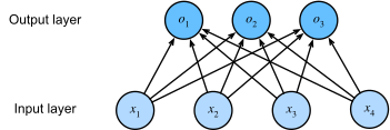
In order to estimate the conditional probabilities associated with all the possible classes, we need a model with multiple outputs, one per class. To address classification with linear models, we will need as many affine functions as we have outputs. Strictly speaking, we only need one fewer, since the final category has to be the difference between \(1\) and the sum of the other categories (indeed, as we will see shortly, only differences of scores end up mattering), but for reasons of symmetry we use a slightly redundant parametrization. Each output corresponds to its own affine function. In our case, since we have 4 features and 3 possible output categories, we need 12 scalars to represent the weights (\(w\) with subscripts), and 3 scalars to represent the biases (\(b\) with subscripts). This yields:
\[ \begin{aligned} o_1 &= x_1 w_{11} + x_2 w_{12} + x_3 w_{13} + x_4 w_{14} + b_1,\\ o_2 &= x_1 w_{21} + x_2 w_{22} + x_3 w_{23} + x_4 w_{24} + b_2,\\ o_3 &= x_1 w_{31} + x_2 w_{32} + x_3 w_{33} + x_4 w_{34} + b_3. \end{aligned} \]
The corresponding neural network diagram is shown in Figure 3.1.1. Just as in linear regression, we use a single-layer neural network. And since the calculation of each output, \(o_1, o_2\), and \(o_3\), depends on every input, \(x_1\), \(x_2\), \(x_3\), and \(x_4\), the output layer can also be described as a fully connected layer.
For a more concise notation we use vectors and matrices: \(\mathbf{o} = \mathbf{W} \mathbf{x} + \mathbf{b}\) is much better suited for mathematics and code. Note that we have gathered all of our weights into a \(3 \times 4\) matrix and all biases \(\mathbf{b} \in \mathbb{R}^3\) in a vector.
3.1.2 The Softmax Model
Assuming a suitable loss function, we could try, directly, to minimize the difference between \(\mathbf{o}\) and the labels \(\mathbf{y}\). While it turns out that treating classification as a vector-valued regression problem can sometimes work, its outputs lack two properties required of probabilities:
- There is no guarantee that the outputs \(o_i\) sum to \(1\) in the way we expect probabilities to behave.
- There is no guarantee that the \(o_i\) are nonnegative, nor that they lie in \([0, 1]\).
Both aspects render the estimation problem difficult to solve and the solution very brittle to outliers. For instance, if we assume that there is a positive linear dependency between the number of bedrooms and the likelihood that someone will buy a house, the probability might exceed \(1\) when it comes to buying a mansion! We therefore need to map the outputs to the probability simplex.
There are many ways we might accomplish this goal. For instance, we could posit that the observed label arises from a noisy argmax: perturb each score by independent noise \(\epsilon_i\) and report the class with the largest perturbed score, \(y = \operatorname*{argmax}_i \, (o_i + \epsilon_i)\). When the noise is Gaussian, \(\epsilon_i \sim \mathcal{N}(0, \sigma^2)\), this is the (multinomial) probit model, first introduced by Fechner (1860) . Compared with softmax, multinomial probit generally lacks a closed-form class probability and leads to a more difficult optimization problem. (Drawing the noise from a Gumbel distribution instead yields exactly the softmax probabilities that we are about to derive.)
Another way to accomplish this goal (and to ensure nonnegativity) is to use an exponential function \(P(y = i) \propto \exp o_i\). This does indeed satisfy the requirement that the conditional class probability increases monotonically with \(o_i\), and all probabilities are nonnegative. We can then transform these values so that they add up to \(1\) by dividing each by their sum. This process is called normalization. Putting these two pieces together gives us the softmax function:
\[\hat{\mathbf{y}} = \mathrm{softmax}(\mathbf{o}) \quad \textrm{where}\quad \hat{y}_i = \frac{\exp(o_i)}{\sum_j \exp(o_j)}. \tag{3.1.2}\]
Note that the largest coordinate of the raw scores \(\mathbf{o}\), also called the logits, corresponds to the most likely class according to \(\hat{\mathbf{y}}\). Moreover, because the softmax operation preserves the ordering among its arguments, we do not need to compute the softmax to determine which class has been assigned the highest probability. Thus,
\[ \operatorname*{argmax}_j \hat y_j = \operatorname*{argmax}_j o_j. \]
For two classes the redundant parametrization noted above becomes explicit. Writing the single logit gap \(o = o_1 - o_2\),
\[\hat{y}_1 = \frac{\exp(o_1)}{\exp(o_1) + \exp(o_2)} = \frac{1}{1 + \exp(-o)} = \sigma(o), \tag{3.1.3}\]
the logistic sigmoid \(\sigma\). Binary logistic regression is thus softmax regression with the redundant logit removed. More generally, adding the same constant \(c\) to every logit, \(o_j \mapsto o_j + c\), multiplies both numerator and denominator of Equation 3.1.2 by \(\exp(c)\) and so leaves \(\hat{\mathbf{y}}\) unchanged: only the differences of logits are identifiable. We may therefore pin one of them, say \(o_q \equiv 0\), without changing any prediction, which is precisely the “one fewer” affine function we alluded to when motivating the linear model. This translation invariance returns in the exercises and underlies the numerically stable implementation.
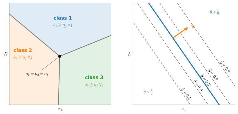
This model has a simple geometry as a classifier (Figure 3.1.2). Since the predicted class is \(\operatorname{argmax}_j o_j\) and each \(o_j = \mathbf{w}_j^\top \mathbf{x} + b_j\) is affine, the region assigned to class \(j\) is the set where finitely many linear inequalities \(o_j \geq o_k\) hold: an intersection of halfspaces, hence a convex polyhedron that may be empty. Pairwise ties \(o_j=o_k\) lie on hyperplanes, although only the portions adjacent to two winning regions are decision boundaries. The three-class example in Figure 3.1.2 has one point where all three scores are equal. With three classes such a common point is in fact the generic case: the three tie hyperplanes \(o_1=o_2\), \(o_2=o_3\), \(o_1=o_3\) are linearly dependent, so in the plane they meet in a single point unless two of them are parallel. With more than three classes in the plane, however, a common intersection is generically impossible. In the binary case the picture is even simpler: \(\hat{y}_1 = \sigma(o)\) depends on \(\mathbf{x}\) only through \(o = (\mathbf{w}_1 - \mathbf{w}_2)^\top \mathbf{x} + (b_1 - b_2)\), so the level sets of the predicted probability are parallel lines perpendicular to \(\mathbf{w}_1 - \mathbf{w}_2\), with the decision boundary at \(\hat{y}_1 = \frac{1}{2}\). Whatever nonlinearity the softmax adds happens in the probabilities, never in the decision boundaries: those stay linear, a limitation we will meet head-on when we train such a model on images.
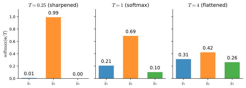
The idea of a softmax dates back to Gibbs (1902), who adapted ideas from physics. Dating even further back, Boltzmann, the father of modern statistical physics, used this trick to model a distribution over energy states in gas molecules. In particular, he discovered that the prevalence of a state of energy in a thermodynamic ensemble, such as the molecules in a gas, is proportional to \(\exp(-E/kT)\). Here, \(E\) is the energy of a state, \(T\) is the temperature, and \(k\) is the Boltzmann constant. When statisticians talk about increasing or decreasing the “temperature” of a statistical system, they refer to changing \(T\) in order to favor lower or higher energy states. Following Gibbs’ idea, energy equates to error. Energy-based models (Ranzato et al. 2007) use this point of view when describing problems in deep learning. In our notation, temperature amounts to replacing \(\mathrm{softmax}(\mathbf{o})\) by \(\mathrm{softmax}(\mathbf{o}/T)\). Figure 3.1.3 shows the effect on one fixed score vector: cooling (\(T < 1\)) sharpens the distribution toward a hard \(\operatorname{argmax}\), heating (\(T > 1\)) flattens it toward uniform, and since \(1/T\) scales every logit alike, the ranking of the classes never changes. We will put this dial to work at the end of the section and in the exercises.
3.1.2.1 Vectorization
To improve computational efficiency, we vectorize calculations in minibatches of data. Assume that we are given a minibatch \(\mathbf{X} \in \mathbb{R}^{n \times d}\) of \(n\) examples with dimensionality (number of inputs) \(d\). Moreover, assume that we have \(q\) categories in the output. Then the weights satisfy \(\mathbf{W} \in \mathbb{R}^{d \times q}\) and the bias satisfies \(\mathbf{b} \in \mathbb{R}^{1\times q}\). Note the layout: with examples stacked in the rows of \(\mathbf{X}\), this \(\mathbf{W}\) is the transpose of the per-example \(\mathbf{W}\) in \(\mathbf{o} = \mathbf{W}\mathbf{x} + \mathbf{b}\) above, so that the product \(\mathbf{X}\mathbf{W}\) pairs each example with its logits row by row.
\[ \begin{aligned} \mathbf{O} &= \mathbf{X} \mathbf{W} + \mathbf{b}, \\ \hat{\mathbf{Y}} & = \mathrm{softmax}(\mathbf{O}). \end{aligned} \tag{3.1.4}\]
This accelerates the dominant operation into a matrix–matrix product \(\mathbf{X} \mathbf{W}\). Moreover, since each row in \(\mathbf{X}\) represents a data example, the softmax operation itself can be computed rowwise: for each row of \(\mathbf{O}\), exponentiate all entries and then normalize them by the sum. Note, though, that care must be taken to avoid exponentiating and taking logarithms of large numbers, since this can cause numerical overflow or underflow: \(\exp(o_k)\) overflows once \(o_k\) is a few hundred, and the small probabilities it produces underflow to \(0\) before we take their logarithm. The standard fix subtracts \(\max_k o_k\) before exponentiating and fuses the softmax and the logarithm into a single log-sum-exp computation; we derive it, and explain why frameworks fold it into the loss and consume raw logits, in Section 3.5.2.
3.1.3 Loss Function
Now that we have a mapping from features \(\mathbf{x}\) to probabilities \(\mathbf{\hat{y}}\), we need a way to optimize the accuracy of this mapping. We will rely on maximum likelihood estimation, the very same method that we encountered when providing a probabilistic justification for the mean squared error loss in Section 2.1.3.
3.1.3.1 Log-Likelihood
The softmax function gives us a vector \(\hat{\mathbf{y}}\), which we can interpret as the (estimated) conditional probabilities of each class, given any input \(\mathbf{x}\), such as \(\hat{y}_1 = P(y=\textrm{cat} \mid \mathbf{x})\). In the following we assume that for a dataset with features \(\mathbf{X}\) the labels \(\mathbf{Y}\) are represented using a one-hot encoding label vector. We can compare the estimates with reality by checking how probable the actual classes are according to our model, given the features:
\[ P(\mathbf{Y} \mid \mathbf{X}) = \prod_{i=1}^n P(\mathbf{y}^{(i)} \mid \mathbf{x}^{(i)}). \]
We are allowed to use the factorization since we assume that each label is drawn independently from its respective distribution \(P(\mathbf{y}\mid\mathbf{x}^{(i)})\). Since maximizing the product of terms is awkward, we take the negative logarithm to obtain the equivalent problem of minimizing the negative log-likelihood:
\[ -\log P(\mathbf{Y} \mid \mathbf{X}) = \sum_{i=1}^n -\log P(\mathbf{y}^{(i)} \mid \mathbf{x}^{(i)}) = \sum_{i=1}^n l(\mathbf{y}^{(i)}, \hat{\mathbf{y}}^{(i)}), \]
where for any pair of label \(\mathbf{y}\) and model prediction \(\hat{\mathbf{y}}\) over \(q\) classes, the loss function \(l\) is
\[ l(\mathbf{y}, \hat{\mathbf{y}}) = - \sum_{j=1}^q y_j \log \hat{y}_j. \tag{3.1.5}\]
For reasons explained later on, the loss function in Equation 3.1.5 is commonly called the cross-entropy loss. Since \(\mathbf{y}\) is a one-hot vector of length \(q\), the sum over all its coordinates \(j\) vanishes for all but one term. Note that the loss \(l(\mathbf{y}, \hat{\mathbf{y}})\) is bounded from below by \(0\) whenever \(\hat{\mathbf{y}}\) is a probability vector: no single entry is larger than \(1\), hence their negative logarithm cannot be lower than \(0\); \(l(\mathbf{y}, \hat{\mathbf{y}}) = 0\) only if we predict the actual label with certainty. This can never happen for any finite setting of the weights because taking a softmax output towards \(1\) requires taking the corresponding input \(o_i\) to infinity (or all other outputs \(o_j\) for \(j \neq i\) to negative infinity). Even if our model could assign an output probability of \(0\), any error made when assigning such high confidence would incur infinite loss (\(-\log 0 = \infty\)).
3.1.3.2 Softmax and Cross-Entropy Loss
Since the softmax function and the corresponding cross-entropy loss are so common, we examine their computation in more detail. Plugging Equation 3.1.2 into the definition of the loss in Equation 3.1.5 and using the definition of the softmax we obtain
\[ \begin{aligned} l(\mathbf{y}, \hat{\mathbf{y}}) &= - \sum_{j=1}^q y_j \log \frac{\exp(o_j)}{\sum_{k=1}^q \exp(o_k)} \\ &= \sum_{j=1}^q y_j \log \sum_{k=1}^q \exp(o_k) - \sum_{j=1}^q y_j o_j \\ &= \log \sum_{k=1}^q \exp(o_k) - \sum_{j=1}^q y_j o_j = g(\mathbf{o}) - \mathbf{y}^\top \mathbf{o}, \end{aligned} \]
using \(\sum_j y_j = 1\) in the last step and writing \(g(\mathbf{o}) = \log \sum_k \exp(o_k)\) for the log-partition function. This is the recurring shape of an exponential-family negative log-likelihood: a convex log-partition term minus a linear term in the natural parameters \(\mathbf{o}\). The derivative is now immediate, because the softmax is the gradient of the log-partition function,
\[ \partial_{o_j} g(\mathbf{o}) = \frac{\exp(o_j)}{\sum_{k=1}^q \exp(o_k)} = \mathrm{softmax}(\mathbf{o})_j, \quad \textrm{hence} \quad \partial_{o_j} l(\mathbf{y}, \hat{\mathbf{y}}) = \mathrm{softmax}(\mathbf{o})_j - y_j. \]
In other words, the derivative is the difference between the probability assigned by our model, as expressed by the softmax operation, and what actually happened, as expressed by elements in the one-hot label vector. In this sense, it is very similar to what we saw in regression, where the two terms were the observation \(y\) and estimate \(\hat{y}\), and the gradient orientation was estimate minus observation. This is not a coincidence: in any exponential-family model the log-likelihood gradient is exactly this “prediction minus observation” residual, which makes the gradient inexpensive to compute; the corresponding negative log-likelihood is convex in \(\mathbf{o}\). The second derivative is the covariance of \(\mathrm{softmax}(\mathbf{o})\), so the Hessian of \(g\) is positive semidefinite. We work this out in the exercises and revisit log-partition convexity in Section 26.3, where the corresponding proposition is proved in full.
Now consider the case where we observe an entire distribution over outcomes rather than a single outcome. We can use the same representation as before for the label \(\mathbf{y}\). The only difference is that rather than a vector containing only binary entries, say \((0, 0, 1)\), we now have a generic probability vector, say \((0.1, 0.2, 0.7)\). The math that we used previously to define the loss \(l\) in Equation 3.1.5 still works well, just that the interpretation is slightly more general. It is the expected value of the loss for a distribution over labels. This loss is called the cross-entropy loss, a commonly used loss for classification problems.
3.1.3.2.1 Why “cross-entropy”?
The name comes from information theory. The entropy \(H[P] = \sum_j -P(j) \log P(j)\) is the expected surprisal \(-\log P(j)\) of draws from \(P\), which Shannon showed is the average number of nats (natural-log units) you must spend to encode them when you know \(P\) (Shannon 1948). The cross-entropy \(H(P, Q) = \sum_j -P(j) \log Q(j)\) is the cost when you instead encode the same draws under a wrong model \(Q\), and it is minimized exactly when \(Q = P\). Our loss Equation 3.1.5 is precisely \(H(\mathbf{y}, \hat{\mathbf{y}})\), so minimizing it does two equivalent things: it maximizes the likelihood of the labels, and it minimizes the excess coding cost of using the predicted distribution rather than the target distribution. We develop entropy, cross-entropy, and the Kullback–Leibler divergence, together with the coding argument behind the “bits” language, in Section 28.1; the classic references are Cover and Thomas (1999) and MacKay (2003).
Confidence is not calibrated probability. We have just seen that the loss keeps rewarding the model for pushing probability onto the correct class even after the decision is already right, so those probabilities should not be read at face value: a model trained to minimize cross-entropy is not necessarily calibrated, and a reported confidence of \(0.9\) does not mean the prediction is right \(90\%\) of the time. Modern deep networks are often empirically overconfident (Guo et al. 2017). A simple and effective remedy is temperature scaling, which divides the logits by a single learned \(T > 0\) before the softmax, exactly the temperature of the Boltzmann distribution in Figure 3.1.3. Because it scales every logit by the same factor \(1/T\) it preserves their order, leaving the predicted class (the \(\operatorname{argmax}\)) and hence the accuracy untouched, while sharpening or softening the confidences. Exercise 8 develops this dial in detail.
3.1.4 Summary and Discussion
This section derived a differentiable loss for a discrete label space. Key in its design was that we took a probabilistic approach, treating discrete categories as instances of draws from a probability distribution. As a side effect, we encountered the softmax, a convenient activation function that transforms outputs of an ordinary neural network layer into valid discrete probability distributions. We saw that the derivative of the cross-entropy loss when combined with softmax behaves very similarly to the derivative of squared error; namely by taking the difference between the expected behavior and its prediction. Along the way we encountered connections to statistical physics (the Boltzmann distribution behind the softmax) and to information theory (cross-entropy as a code length), the latter taken up in Section 28.1.
The resulting chain is the one used throughout the chapter: affine logits, softmax probabilities, categorical likelihood, cross-entropy, and the residual gradient \(\hat{\mathbf y}-\mathbf y\). Computational approximations for very large output spaces are treated with the systems and large-vocabulary models for which they are needed.
3.1.5 Exercises
- Softmax Hessian. Write the cross-entropy loss as a function of the logits, \(l(\mathbf{y}, \mathbf{o}) = g(\mathbf{o}) - \mathbf{y}^\top \mathbf{o}\) with \(g(\mathbf{o}) = \log \sum_k \exp(o_k)\), as in
Section 3.1.3.2.
- Compute the Hessian \(\partial^2_{\mathbf{o}}\, l(\mathbf{y}, \mathbf{o})\) and show that it does not depend on \(\mathbf{y}\).
- Let \(\mathbf{e}_Y\) be the one-hot vector of a class \(Y\) drawn from \(\mathrm{softmax}(\mathbf{o})\). Compute the covariance matrix of \(\mathbf{e}_Y\) and show that it equals the Hessian from the previous step.
- Conclude that \(g\) is convex and that the cross-entropy loss is convex in the logits.
- Softmax and sigmoid. By Equation 3.1.3, binary logistic regression is softmax regression with the redundant logit removed. A colleague hands you a fitted binary logistic model \(P(y = 1 \mid x) = \sigma(\hat\beta_0 + \hat\beta_1 x)\) with \(\hat\beta_0 = 2\) and \(\hat\beta_1 = -1\).
- Characterize all two-class softmax coefficients \((w_1, b_1)\) and \((w_2, b_2)\) whose predictions coincide with the logistic model for every \(x\), and identify the pair with \(o_2 \equiv 0\).
- Show that gradient descent on the cross-entropy loss of the two-class softmax model never changes \(w_1 + w_2\) or \(b_1 + b_2\). Suppose that gradient descent starts from \(w_1 = w_2 = b_1 = b_2 = 0\) on the colleague’s training data and converges to coefficients that reproduce the logistic model. Determine which pair it reaches.
- Coding three classes. Assume that we have three classes which occur with equal probability, i.e., the probability vector is \(P = (1/3, 1/3, 1/3)\), whose entropy is \(\log_2 3 \approx 1.585\) bits. See Section 28.1 for the information-theoretic background.
- A fixed-length binary code, in which every codeword has the same number of bits, needs \(2\) bits for a single observation. Design a fixed-length binary code for blocks of \(n\) independent observations. Find the smallest \(n\) for which it uses fewer than \(2\) bits per observation, and show that the per-observation rate approaches \(\log_2 3\) bits as \(n\) grows.
- The variable-length code \(\{0, 10, 11\}\) for a single observation is optimal for the distribution \(Q = (1/2, 1/4, 1/4)\). Compute its expected length in bits when observations are drawn from \(P\), and compare it with the entropy of \(P\) and with the cross-entropy \(H(P, Q)\) in bits.
- Separable data. ● Suppose that some parameters \((\mathbf{W}, \mathbf{b})\) classify every training example correctly and without ties: on each example, the logit of the true class strictly exceeds every other logit. Consider the scaled parameters \((c\mathbf{W}, c\mathbf{b})\) for \(c > 0\).
- Show that the cross-entropy loss of every training example strictly decreases as \(c\) grows and tends to \(0\) as \(c \to \infty\).
- Conclude that the training loss has no minimizer and that every sequence of parameters whose training loss tends to \(0\) has unbounded norm.
- Add the weight decay penalty of Section 2.7, applied to both weights and biases, \(\frac{\lambda}{2}(\|\mathbf{W}\|^2 + \|\mathbf{b}\|^2)\) with \(\lambda > 0\), to the training loss. Show that the penalized loss has a minimizer.
- Bradley–Terry model. The Bradley–Terry model (Bradley and Terry 1952) uses a logistic model to capture preferences. A user who chooses between apples and oranges picks each item with the probability given by the softmax of two scores, \(o_{\textrm{apple}}\) and \(o_{\textrm{orange}}\). Now add a default option of choosing neither, with a fixed score \(o_{\textrm{none}} = 0\).
- Determine whether adding the same constant to \(o_{\textrm{apple}}\) and \(o_{\textrm{orange}}\) changes the choice probabilities, first without and then with the default option. Conclude which scores the observed choices can determine in each model.
- Compare the ratio \(P(\textrm{apple}) / P(\textrm{orange})\) with and without the default option. Describe a choice situation in which real users would not keep this ratio fixed.
- RealSoftMax. The log-sum-exp function \(\textrm{RealSoftMax}(a, b) = \log (\exp(a) + \exp(b))\) is the log-partition function \(g\) of Section 3.1.3.2 in two arguments, so its gradient is the softmax of \((a, b)\).
- Prove that \[\max(a, b) < \textrm{RealSoftMax}(a, b) \leq \max(a, b) + \log 2, \tag{3.1.6}\] with equality on the right exactly when \(a = b\), and show that the gap to \(\max(a, b)\) can be made arbitrarily small. Hint: without loss of generality set \(b = 0\) and \(a \geq 0\).
- Prove that for every \(\lambda > 0\) \[\max(a, b) < \lambda^{-1} \textrm{RealSoftMax}(\lambda a, \lambda b) \leq \max(a, b) + \lambda^{-1} \log 2, \tag{3.1.7}\] and conclude that \(\lambda^{-1} \textrm{RealSoftMax}(\lambda a, \lambda b) \to \max(a, b)\) as \(\lambda \to \infty\).
- Construct an analogous softmin function.
- Extend the definition and both bounds to \(q\) numbers, showing that the gap to \(\max_i a_i\) is at most \(\log q\).
- Log-partition function. The function \(g(\mathbf{x}) \stackrel{\textrm{def}}{=} \log \sum_i \exp x_i\) is sometimes also referred to as the log-partition function. Evaluated as written, \(g\) overflows when some \(x_i\) is large, and it returns \(\log 0 = -\infty\) when all \(x_i\) are strongly negative, because every \(\exp x_i\) underflows to \(0\).
- Show that \(g\) is translation equivariant, i.e., \(g(\mathbf{x} + b \mathbf{1}) = b + g(\mathbf{x})\).
- Show that evaluating \(g(\mathbf{x})\) as \(g(\mathbf{x} - \bar{x}\mathbf{1}) + \bar{x}\) with \(\bar{x} = \max_i x_i\) neither overflows nor loses the leading term to underflow.
- Temperature. Recall from Figure 3.1.3 that changing the temperature of \(P = \mathrm{softmax}(\mathbf{o})\) amounts to replacing \(\mathrm{softmax}(\mathbf{o})\) by \(\mathrm{softmax}(\mathbf{o}/T)\). Suppose we pick another distribution \(Q\) with \(Q(i) \propto P(i)^\alpha\) for \(\alpha > 0\).
- Which choice of \(\alpha\) corresponds to doubling the temperature? Which choice corresponds to halving it?
- Suppose that exactly \(m\) of the \(q\) logits attain the largest value. Find the limit of \(\mathrm{softmax}(\mathbf{o}/T)\) as \(T \to 0\).
- Let \(\bar{o} = \frac{1}{q}\sum_j o_j\) be the mean logit. Show that for large \(T\) \[\mathrm{softmax}(\mathbf{o}/T)_i = \frac{1}{q} + \frac{o_i - \bar{o}}{qT} + O(T^{-2}). \tag{3.1.8}\]
- Temperature scaling fits a single \(T\) by minimizing the cross-entropy on a held-out set with the classifier’s logits held fixed. Show that this cross-entropy is a convex function of \(\beta = 1/T\), so that the fit is a one-dimensional convex problem. Hint: use the convexity of the log-partition function \(g\) from exercise 1.
- [code] Gumbel-max trick. ● Section 3.1.2 modeled an observed label as a noisy argmax, \(y = \operatorname*{argmax}_i \, (o_i + \epsilon_i)\). Gaussian noise gives the probit model, whose class probabilities have no closed form; one other noise distribution reproduces the softmax probabilities exactly. Let \(\gamma_1, \ldots, \gamma_q\) be i.i.d. draws from the standard Gumbel distribution, whose CDF is \(P(\gamma \leq z) = \exp(-\exp(-z))\).
- Show that \(P(o_k + \gamma_k \leq z) = \exp(-\exp(o_k)\exp(-z))\).
- Show that \(P\left(\operatorname{argmax}_i \, (o_i + \gamma_i) = k\right) = \mathrm{softmax}(\mathbf{o})_k\). Hint: condition on the value of \(o_k + \gamma_k\) and use the substitution \(u = \exp(-z)\).
- Conclude that scaling the noise, \(\gamma_i \mapsto T\gamma_i\), samples from \(\mathrm{softmax}(\mathbf{o}/T)\).
- Verify your result numerically: for \(\mathbf{o} = (1.0, 2.2, 0.3)\) and \(T \in \{0.25, 1, 4\}\), draw \(10^5\) samples of \(\operatorname{argmax}_i (o_i + T\gamma_i)\) and confirm that the label frequencies match \(\mathrm{softmax}(\mathbf{o}/T)\) up to Monte Carlo error.