%matplotlib inline
from d2l import torch as d2l
import time
import torch
from torch.nn import functional as F
from torch.profiler import ProfilerActivity, profile11.7 Scaling Laws and Current Transformer Configurations
The models in this chapter use the same blocks and training objectives as much larger deployed models, but differ greatly in parameter count, data, and computation. Section 9.11 studied how hyperparameters transfer between model sizes. Here we instead ask how performance changes with scale and how a fixed training budget should be allocated between parameters and data. We derive the \(6ND\) approximation for training cost and compare it with a profiler, conduct a small scaling experiment on one GPU, and summarize the configurations reported for several 2023–2025 open-weight models.
%matplotlib inline
from d2l import jax as d2l
from flax import nnx
import jax
from jax import numpy as jnp
import optax
11.7.1 Counting Parameters and FLOPs
11.7.1.1 Counting Parameters
A GPT holds two kinds of parameters, and they scale differently. The blocks hold \(12d^2\) each — \(4d^2\) of attention, \(8d^2\) of feed-forward network, however the activation slices it (Section 11.1) — for about \(12Ld^2\) across \(L\) blocks. The embedding holds \(Vd\) for a vocabulary of size \(V\), used twice thanks to weight tying but stored once; a learned position table adds another \(\textrm{max\_len} \times d\). The census below runs the accounting on our default configuration and on the GPT-2 configuration from Section 11.2:
count = lambda m: sum(p.numel() for p in m.parameters())

def census(model, d, num_blks):
    emb = count(model.token_emb) + (
        count(model.pos_emb) if model.pos == 'learned' else 0)
    total = count(model)
    print(f'embedding {emb / 1e6:6.2f}M ({emb / total:4.0%}),  '
          f'blocks {(total - emb) / 1e6:6.2f}M '
          f'= {(total - emb) / (num_blks * d ** 2):.2f} L d^2,  '
          f'total {total / 1e6:.2f}M')

census(d2l.GPT(vocab_size=28), d=256, num_blks=6)
census(d2l.GPT(vocab_size=50257, num_hiddens=768, num_heads=12,
               num_blks=12, pos='learned', norm='layer', act='gelu',
               bias=True), d=768, num_blks=12)
embedding 0.01M ( 0%), blocks 4.72M = 12.01 L d^2, total 4.73M
embedding 39.38M ( 32%), blocks 85.06M = 12.02 L d^2, total 124.44Mcount = lambda m: sum(
p.size for p in jax.tree.leaves(nnx.state(m, nnx.Param)))
def census(model, d, num_blks):
emb = count(model.token_emb) + (
count(model.pos_emb) if model.pos == 'learned' else 0)
total = count(model)
print(f'embedding {emb / 1e6:6.2f}M ({emb / total:4.0%}), '
f'blocks {(total - emb) / 1e6:6.2f}M '
f'= {(total - emb) / (num_blks * d ** 2):.2f} L d^2, '
f'total {total / 1e6:.2f}M')
census(d2l.GPT(vocab_size=28), d=256, num_blks=6)
census(d2l.GPT(vocab_size=50257, num_hiddens=768, num_heads=12,
num_blks=12, pos='learned', norm='layer', act='gelu',
bias=True), d=768, num_blks=12)embedding 0.01M ( 0%), blocks 4.72M = 12.01 L d^2, total 4.73M
embedding 39.38M ( 32%), blocks 85.06M = 12.02 L d^2, total 124.44MBoth rows confirm the \(12Ld^2\) rule to a fraction of a percent (the residue is normalization weights and, for GPT-2, biases). The interesting column is the embedding share: negligible for our character model with its 28 symbols, but nearly a third of GPT-2. Comparing \(Vd\) against \(12Ld^2\) says the embedding dominates when \(V \gtrsim 12Ld\) — small models with real vocabularies. GPT-2’s “124M parameters” is in this sense a generous description of an 85M-parameter transformer attached to a 39M-parameter lookup table. Scaling-law papers accordingly count non-embedding parameters (Kaplan et al. 2020): the embedding’s size tracks the tokenizer’s vocabulary, not the computation each token receives, and including it bends the low-end of every curve for accounting reasons rather than scientific ones. We adopt the same convention; \(N\) below means non-embedding parameters.
11.7.1.2 Six FLOPs per Parameter and Token
The approximation below counts matrix multiplications whose arithmetic scales with the model parameters. It excludes attention-score and value-mixing operations, which depend on context length even though they add no parameters. For a context of \(n\) tokens, those operations add about \(4nd\) FLOPs per token per layer, compared with approximately \(24d^2\) from the block’s linear maps. The omitted-to-counted ratio is therefore about \(n/(6d)\): 8% at \(n=128\) and \(d=256\), and no longer small when \(n\) approaches \(6d\).
Multiplying one token’s activation vector by a weight matrix \(\mathbf{W} \in \mathbb{R}^{m \times n}\) takes \(mn\) multiply–add pairs: 2 FLOPs per parameter, so a forward pass costs about \(2N\) per token. The backward pass costs twice the forward: each linear layer must produce two gradients, one with respect to its input (\(\mathbf{W}^\top \boldsymbol{\delta}\), to keep the chain rule moving) and one with respect to its weights (\(\boldsymbol{\delta} \mathbf{x}^\top\), to learn), and each is a matrix multiply of the same size as the forward one. Training on \(D\) tokens therefore costs
\[ C \approx \underbrace{2ND}_{\textrm{forward}} + \underbrace{4ND}_{\textrm{backward}} = 6ND \tag{11.7.1}\]
floating-point operations (Kaplan et al. 2020). This is training arithmetic; the corresponding decode-time accounting — why generating a token costs about \(2N\) and why the KV cache turns generation into a memory problem rather than a compute one — was the business of Section 11.3.
Normalization, softmax, and optimizer updates add further operations not represented by \(6ND\). Thus the formula is a leading estimate for dense transformers in the regime \(n\ll6d\), not an exact operation count. It places the teaching run of Section 11.2 near \(5\times10^{14}\) FLOPs under this accounting convention; profiler comparisons below quantify the discrepancy.
11.7.1.3 Checking the Arithmetic
We compare the approximation with framework operation counts.
PyTorch’s profiler attributes FLOPs to the operations it recognizes — above all the aten::mm matrix multiplies behind every linear layer. The fused attention kernel keeps its score arithmetic to itself and reports none, so the profiler and Equation 11.7.1 ignore the same subleading term. For the count, \(N\) plus the tied output head is exactly the 2-D parameters of the RoPE configuration. The embedding participates in matrix multiplication as the head, whereas the lookup itself contributes no counted FLOPs.
XLA can price a program without running it: lowering the jitted training step and asking the compiled artifact for its cost_analysis() returns an exact operation count of the optimized computation, attention scores and softmax included. One quirk dictates our flags: with act='swiglu' the matched-budget width \(\mathrm{round}(8d/3) = 683\) sends one FFN matrix multiply down a code path whose work the analyzer does not count, underreporting the FFN by a third. The GELU configuration keeps every matrix a round size and is counted exactly, at the same parameter budget, so that is the one we lower. For the count, \(N\) plus the tied output head is exactly the 2-D parameters of the model.
device = d2l.try_gpu()
model = d2l.GPT(vocab_size=28).to(device)
X = torch.randint(0, 28, (64, 128), device=device)
Y = torch.randint(0, 28, (64, 128), device=device)
N = sum(p.numel() for p in model.parameters() if p.ndim == 2)

def train_step():
    loss = F.cross_entropy(model(X).flatten(0, 1), Y.flatten())
    model.zero_grad()
    loss.backward()

for _ in range(3):
    train_step()                    # warm up
with profile(activities=[ProfilerActivity.CPU, ProfilerActivity.CUDA],
             with_flops=True) as prof:
    train_step()
measured = sum(e.flops for e in prof.key_averages() if e.flops)
print(f'6ND analytic: {6 * N * X.numel():.3e} FLOPs')
print(f'profiler:     {measured:.3e} FLOPs '
      f'(ratio {measured / (6 * N * X.numel()):.3f})')
if device.type == 'cuda':
    torch.cuda.synchronize()
t0 = time.time()
for _ in range(20):
    train_step()
if device.type == 'cuda':
    torch.cuda.synchronize()
dt = (time.time() - t0) / 20
print(f'{dt * 1e3:.0f} ms per step: '
      f'{6 * N * X.numel() / dt / 1e12:.1f} TFLOP/s achieved')
6ND analytic: 2.324e+11 FLOPs
profiler: 2.326e+11 FLOPs (ratio 1.001)
21 ms per step: 11.0 TFLOP/s achievedmodel = d2l.GPT(vocab_size=28, act='gelu', rngs=nnx.Rngs(0))
key_x, key_y = jax.random.split(jax.random.key(0))
X = jax.random.randint(key_x, (64, 128), 0, 28)
Y = jax.random.randint(key_y, (64, 128), 0, 28)
graphdef, params, rest = nnx.split(model, nnx.Param, ...)
N = sum(p.size for p in jax.tree.leaves(params) if p.ndim == 2)
def loss_fn(params, X, Y):
logits = nnx.merge(graphdef, params, rest)(X)
return optax.softmax_cross_entropy_with_integer_labels(
logits.reshape(-1, logits.shape[-1]), Y.reshape(-1)).mean()
fwd = jax.jit(loss_fn).lower(params, X, Y).compile().cost_analysis()
both = jax.jit(jax.value_and_grad(loss_fn)).lower(
params, X, Y).compile().cost_analysis()
print(f'2ND analytic: {2 * N * X.size:.3e} FLOPs, '
f'XLA forward: {fwd["flops"]:.3e} '
f'(ratio {fwd["flops"] / (2 * N * X.size):.2f})')
print(f'6ND analytic: {6 * N * X.size:.3e} FLOPs, '
f'XLA step: {both["flops"]:.3e} '
f'(ratio {both["flops"] / (6 * N * X.size):.2f})')
print(f'backward / forward = '
f'{(both["flops"] - fwd["flops"]) / fwd["flops"]:.2f}')2ND analytic: 7.743e+10 FLOPs, XLA forward: 8.480e+10 (ratio 1.10)
6ND analytic: 2.323e+11 FLOPs, XLA step: 2.547e+11 (ratio 1.10)
backward / forward = 2.00Both authorities side with the formula. The PyTorch profiler’s count agrees with \(6ND\) to a fraction of a percent — matching so tightly only because both books omit the fused attention kernel’s score work. XLA’s static analysis, which counts everything, lands about ten percent above \(6ND\), right where the \(n/(6d)\) correction plus softmax and normalization put it, and splits forward to backward at almost exactly one to two: the derivation’s 2-plus-4, read off a compiler’s ledger. The timing line adds a practical limitation: our achieved throughput is roughly an order of magnitude below what the GPU can deliver, because a model this small cannot keep the hardware fully utilized. Production runs choose widths and batch sizes to increase utilization, which favors larger matrix operations.
11.7.2 A Miniature Scaling Study
Counting determines the cost of a run but not its resulting performance. A scaling law describes the empirical regularity that budgets are planned: across many orders of magnitude, language-model loss falls as a power law in each of model size, data, and compute, provided none of the three is the bottleneck (Kaplan et al. 2020). On log-log axes a power law is a straight line. Within a validated regime, fitted lines can support compute planning; extrapolation beyond that regime requires new evidence. The Chinchilla study asked how to split a fixed compute budget between \(N\) and \(D\). Under its model family, data mixture, optimizer, and FLOP accounting, the fitted allocation grew parameters and tokens at similar rates and placed the optimum near twenty training tokens per parameter (Hoffmann et al. 2022). Its 70B-parameter model, trained on 1.4 trillion tokens, outperformed the study’s 280B-parameter comparison trained on 300 billion tokens at matched estimated compute. The ratio and ranking are results of that protocol rather than universal constants.
The following fixed-data experiment illustrates a possible departure from a straight log–log trend. It does not reproduce the Chinchilla fit.
11.7.2.1 Constructing the Training Corpus
Section 11.2 already showed what a too-small corpus does: 4.7M parameters against 180 KB of Wells bottomed out their validation loss within a few hundred steps and spent the rest of the run memorizing. Our own preliminary check confirms the diagnosis for the whole size range: on The Time Machine alone, every configuration beyond about \(10^5\) parameters is saturated more or less immediately. A scaling study needs a corpus large enough to distinguish the configurations. We use the Penn Treebank training text (5 MB of Wall Street Journal prose that Section 18.4 uses for word vectors) concatenated onto the novel. The subclass below reuses the entire character pipeline of d2l.TimeMachine and changes two things: _download returns the concatenated text, and the windows stride by num_steps instead of overlapping (five million overlapping windows would be a five-gigabyte tensor for no statistical gain). One cosmetic note: PTB ships pre-tokenized, with rare words replaced by <unk> and numbers by N, which the character pipeline renders as the literal words unk and n — harmless static for a character model.
class ScalingCorpus(d2l.TimeMachine):
    """Character corpus: The Time Machine plus the PTB training text."""
    def _download(self):
        data_dir = d2l.download_extract('ptb')
        with open(f'{data_dir}/ptb.train.txt') as f:
            ptb = f.read()
        return super()._download() + ' ' + ptb

    def __init__(self, batch_size, num_steps, num_val=2000):
        d2l.DataModule.__init__(self)
        self.save_hyperparameters()
        corpus, self.vocab = self.build(self._download())
        array = d2l.tensor([corpus[i:i + num_steps + 1] for i in
                            range(0, len(corpus) - num_steps, num_steps)])
        self.X, self.Y = array[:, :-1], array[:, 1:]
        self.num_train = len(array) - num_val

data = ScalingCorpus(batch_size=64, num_steps=128)
print(f'{len(data.X) * 128 / 1e6:.1f}M characters in {len(data.X)} '
      f'windows, vocabulary size {len(data.vocab)}')
5.1M characters in 39491 windows, vocabulary size 28class ScalingCorpus(d2l.TimeMachine):
"""Character corpus: The Time Machine plus the PTB training text."""
def _download(self):
data_dir = d2l.download_extract('ptb')
with open(f'{data_dir}/ptb.train.txt') as f:
ptb = f.read()
return super()._download() + ' ' + ptb
def __init__(self, batch_size, num_steps, num_val=2000):
d2l.DataModule.__init__(self)
self.save_hyperparameters()
corpus, self.vocab = self.build(self._download())
array = d2l.tensor([corpus[i:i + num_steps + 1] for i in
range(0, len(corpus) - num_steps, num_steps)])
self.X, self.Y = array[:, :-1], array[:, 1:]
self.num_train = len(array) - num_val
data = ScalingCorpus(batch_size=64, num_steps=128)
print(f'{len(data.X) * 128 / 1e6:.1f}M characters in {len(data.X)} '
f'windows, vocabulary size {len(data.vocab)}')5.1M characters in 39491 windows, vocabulary size 28The 5.1-million-character corpus is small enough to expose repeated-data effects within a short experiment. We compare non-embedding parameter counts from 0.33M to 14.2M while holding token exposure fixed. This range is chosen to show where validation improvements may diminish; it is not derived from a universal tokens-per-parameter rule.
11.7.2.2 Comparing Five Model Sizes
The design: hold the data fixed and move only the model. Five sizes of d2l.GPT, widths 96 to 384 and depths 3 to 8 grown together the way real model families grow, spanning 0.33M to 14.2M non-embedding parameters — about a factor of forty. Every size consumes an identical diet of 16.4M tokens (2,000 steps of 64 sequences of 128 characters), roughly three passes over the corpus. Dropout is zero: it was a small-corpus crutch in Section 11.2, this experiment is about the corpus running out, and the recipe table below will show that models whose corpora outweigh their parameters do not use it either. The one hyperparameter that must not be held fixed is the learning rate: Section 9.11 showed that the tuned optimum drifts with width, and a rate frozen at any single value would handicap one end of the family (our pilot grid confirmed it at both ends). We apply that section’s transfer rule instead of re-tuning: anchor at \(10^{-3}\) for width 256 and scale inversely with width. One seeded run per size; rerunning a point with a different seed moves it by less than a hundredth of a nat, well below the structure we are about to read.
def val_loss(model, data):
    model.to(device).eval()
    with torch.no_grad():
        losses = [F.cross_entropy(
            model(X.to(device)).flatten(0, 1), Y.to(device).flatten())
            for X, Y in data.val_dataloader()]
    model.train()
    return sum(l.item() for l in losses) / len(losses)

sizes = ((96, 3, 4), (128, 3, 4), (192, 4, 6), (256, 6, 8), (384, 8, 8))
Ns, curves = [], {'train': [], 'validation': []}
for d, num_blks, num_heads in sizes:
    torch.manual_seed(0)
    model = d2l.GPT(len(data.vocab), num_hiddens=d, num_heads=num_heads,
                    num_blks=num_blks, dropout=0)
    optimizer = torch.optim.AdamW(model.parameters(), lr=1e-3 * 256 / d,
                                  weight_decay=0.0)
    losses = d2l.train_lm(model, data, optimizer, 2000)
    Ns.append(count(model) - count(model.token_emb))
    curves['train'].append(sum(losses[-50:]) / 50)
    curves['validation'].append(val_loss(model, data))
    print(f'd={d:3d}, {num_blks} blocks: {Ns[-1] / 1e6:5.2f}M parameters, '
          f'train {curves["train"][-1]:.2f}, '
          f'validation {curves["validation"][-1]:.2f}')
d= 96, 3 blocks: 0.33M parameters, train 1.21, validation 1.20
d=128, 3 blocks: 0.59M parameters, train 1.17, validation 1.17
d=192, 4 blocks: 1.77M parameters, train 1.11, validation 1.12
d=256, 6 blocks: 4.72M parameters, train 1.06, validation 1.09
d=384, 8 blocks: 14.16M parameters, train 1.03, validation 1.06@nnx.jit
def batch_loss(model, X, Y):
logits = model(X)
return optax.softmax_cross_entropy_with_integer_labels(
logits.reshape(-1, logits.shape[-1]), Y.reshape(-1)).mean()
def val_loss(model, data):
model.eval()
losses = [float(batch_loss(model, jnp.asarray(X), jnp.asarray(Y)))
for X, Y in data.val_dataloader()]
model.train()
return sum(losses) / len(losses)
sizes = ((96, 3, 4), (128, 3, 4), (192, 4, 6), (256, 6, 8), (384, 8, 8))
Ns, curves = [], {'train': [], 'validation': []}
for d, num_blks, num_heads in sizes:
model = d2l.GPT(len(data.vocab), num_hiddens=d, num_heads=num_heads,
num_blks=num_blks, dropout=0, rngs=nnx.Rngs(0))
optimizer = nnx.Optimizer(
model, optax.adamw(1e-3 * 256 / d, weight_decay=0.0),
wrt=nnx.Param)
losses = d2l.train_lm(model, data, optimizer, 2000)
Ns.append(count(model) - count(model.token_emb))
curves['train'].append(sum(losses[-50:]) / 50)
curves['validation'].append(val_loss(model, data))
print(f'd={d:3d}, {num_blks} blocks: {Ns[-1] / 1e6:5.2f}M parameters, '
f'train {curves["train"][-1]:.2f}, '
f'validation {curves["validation"][-1]:.2f}')d= 96, 3 blocks: 0.33M parameters, train 1.21, validation 1.21
d=128, 3 blocks: 0.59M parameters, train 1.17, validation 1.17
d=192, 4 blocks: 1.77M parameters, train 1.11, validation 1.12
d=256, 6 blocks: 4.72M parameters, train 1.06, validation 1.08
d=384, 8 blocks: 14.16M parameters, train 1.04, validation 1.07d2l.plot(Ns, [curves['train'], curves['validation']],
'parameters $N$ (non-embedding)', 'loss',
legend=['train', 'validation'], xscale='log', yscale='log',
fmts=('o-', 's--'))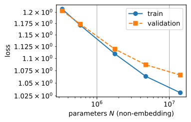
d2l.plot(Ns, [curves['train'], curves['validation']],
         'parameters $N$ (non-embedding)', 'loss',
         legend=['train', 'validation'], xscale='log', yscale='log',
         fmts=('o-', 's--'))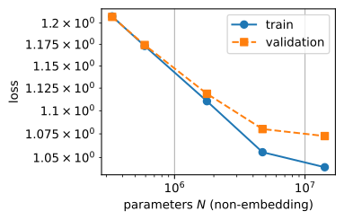
11.7.2.3 Interpreting the Departure from a Power Law
The smaller models lie approximately along a straight segment on the log–log plot. The largest model shows a smaller validation improvement than an extrapolation from that segment, while its training loss continues to fall. This widening train–validation gap is consistent with a fixed-data limitation after three passes through the 5.1-million-character corpus. Other explanations, including model-specific optimization and hyperparameter effects, are not excluded by this sweep.
This five-size, one-seed experiment is a qualitative demonstration of how a fixed corpus can limit gains from additional parameters. It cannot estimate a power-law exponent, an irreducible loss, or a compute-optimal token–parameter ratio. Those quantities in the next subsection come from the multi-model, multi-data fits of Kaplan et al. (2020); Hoffmann et al. (2022), not from our curve. Repeated-data studies further show that the value of additional passes depends on repetition count and data conditions (Muennighoff et al. 2023).
Two footnotes before trusting the plot. First, a scaling study is only as good as the tuning of each point: had we frozen the learning rate across widths, part of our “bend” would have been a tuning artifact (Section 9.11; exercise 9 has you produce this artifact deliberately). Second, loss is the quantity that scales smoothly; downstream abilities can surface abruptly as loss creeps down, which is why small differences on this axis are worth more than they look (Wei et al. 2022).
11.7.2.4 The Published Form of the Law
Our miniature moved \(N\) with \(D\) pinned; the published fits treat both as free variables. Across more than four hundred training runs, Hoffmann et al. (2022) fit the loss surface
\[ L(N, D) = E + \frac{A}{N^{\alpha}} + \frac{B}{D^{\beta}}, \tag{11.7.2}\]
Here \(E\) is a fitted asymptotic floor under the study’s data distribution and loss definition; \(A/N^{\alpha}\) and \(B/D^{\beta}\) describe fitted parameter- and data-limited contributions. With \(D\) fixed, the latter two terms predict diminishing gains from increasing \(N\). This is qualitatively consistent with our largest-model result, but our five points do not identify any of the terms or show that this law caused the observed bend.
Compute-optimal allocation drops out of Equation 11.7.2 with one constraint. Fix a budget \(C \approx 6ND\), substitute \(D = C/6N\), and set the derivative in \(N\) to zero: the optimum satisfies
\[ \alpha \frac{A}{N^{\alpha}} = \beta \frac{B}{D^{\beta}}, \tag{11.7.3}\]
i.e., spend until the two shrinkable terms are shrinking at equal marginal rates. Solving gives \(N^* \propto C^{\beta/(\alpha+\beta)}\) and \(D^* \propto C^{\alpha/(\alpha+\beta)}\). The fitted exponents come out nearly equal (\(\alpha \approx 0.34\), \(\beta \approx 0.28\)), so both optima scale close to \(C^{1/2}\): parameters and tokens should grow in near-lockstep. In the models, data mixture, optimizer, and FLOP accounting of Hoffmann et al. (2022), the fitted allocation was approximately twenty training tokens per parameter. This is a result for that protocol, not a portable constant; data quality, repeated data, model family, and accounting conventions can shift the allocation. We do not fit \(E\), \(\alpha\), \(\beta\) to our own five points (the previous subsection said why); what the miniature contributes is the shape of both terms — the straight stretch is \(A/N^{\alpha}\) falling while the data term is negligible, and the bend is the crossover where the fixed corpus’s \(B/D^{\beta}\) takes over.
11.7.3 Reported Transformer Configurations, 2023–2025
Architectural reports for large training runs can be compared along the interfaces developed in this chapter. Table 11.7.1 compiles the architecture sections of seven open-weights families onto the axes this chapter built: Mistral 7B (Jiang et al. 2023), Llama 3 (Grattafiori et al. 2024), Qwen3 (Yang et al. 2025), OLMo 2 and 3 (Team OLMo et al. 2025; Team OLMo 2025), DeepSeek-V3 (DeepSeek-AI et al. 2024), Gemma 3 (Gemma Team 2025), and GPT-OSS (OpenAI 2025).
11.7.3.1 Common Architectural Choices
| model | attention and cache | normalization | positions | FFN | dense or MoE | dropout |
|---|---|---|---|---|---|---|
| Mistral 7B (2023) | GQA \(32{:}8\); sliding window 4096 | RMSNorm, pre | RoPE, \(\theta = 10^4\) | SwiGLU | dense | none |
| Llama 3 (2024) | GQA \(32{:}8\) | RMSNorm, pre | RoPE, \(\theta = 5 \times 10^5\) | SwiGLU | dense | none |
| Qwen3 (2025) | GQA: \(64{:}8\) dense (32B), \(64{:}4\) MoE (235B-A22B) | RMSNorm, pre; QK-norm | RoPE, \(\theta = 10^6\); YaRN for long context | SwiGLU | dense, and MoE: 128 experts, 8 active | none |
| OLMo 2/3 (2024/25) | MHA (7B), GQA (32B); OLMo 3: window 4096 on 3 of 4 layers | RMSNorm, post but off-stream; QK-norm | RoPE | SwiGLU | dense | none |
| DeepSeek-V3 (2024) | MLA: KV compressed to a 512-dim latent | RMSNorm, pre | RoPE on a decoupled 64-dim slice per head | SwiGLU | MoE: 256 experts plus 1 shared, 8 active | none |
| Gemma 3 (2025) | GQA; local:global \(5{:}1\), window 1024 | RMSNorm, pre and post; QK-norm | RoPE, \(\theta = 10^6\) global, \(10^4\) local | GeGLU | dense | none |
| GPT-OSS (2025) | GQA \(64{:}8\); window 128 on alternate layers; learned sinks | RMSNorm, pre | RoPE; YaRN | SwiGLU, clamped | MoE: 128 or 32 experts, 4 active | none |
Read down the columns and the convergence is hard to miss. Every row is the block of Section 11.1 in the causal wiring of Section 11.2; nothing here is a new architecture in the sense that the transformer was new against the LSTM. The differences cluster on exactly three axes. Stability: where the norms sit and what they normalize, with pre-norm almost everywhere, RMSNorm everywhere, QK-norm spreading through the 2025 column (OLMo’s post-but-off-stream placement is the one live dissent, and it concedes the residual stream’s identity path, the actual lesson of our signal-propagation experiment). The cache: GQA as the default, with the window-plus-sink and latent compressions of Section 11.3 where long contexts make the cache the binding cost. Capacity per FLOP: gated FFNs in every row, and mixture of experts (Section 11.6) where the budget wants more parameters than FLOPs. The dropout column also follows from the scaling regime: at trillion-token scale the corpus outweighs the parameters, overfitting is not the failure mode, and the regularizer used in Section 11.2 is omitted. Even the positions column is one idea at different dial settings: RoPE with an inflated base for longer contexts, stretched further by interpolation schemes (Section 10.4); the newest twist is still a setting of the same dial, dropping positions entirely on some layers as Llama 4’s NoPE-interleaved long-context layers do.
11.7.3.2 Expressing Configurations as Constructor Calls
Section 11.2 represented architectural choices as constructor arguments. At width 256 and six blocks — here are four rows of the table as configurations of d2l.GPT, with grouped-query attention dropped in through the same seam Section 11.3 built:
recipes = {
    'GPT-2 (2019)': dict(pos='learned', norm='layer', act='gelu',
                         pre_norm=True, bias=True, kv_heads=8),
    'Mistral-7B':   dict(pos='rope', norm='rms', act='swiglu',
                         pre_norm=True, bias=False, kv_heads=2),
    'Llama-3':      dict(pos='rope', norm='rms', act='swiglu',
                         pre_norm=True, bias=False, kv_heads=2),
    'Qwen3':        dict(pos='rope', norm='rms', act='swiglu',
                         pre_norm=True, bias=False, kv_heads=2),
}
for name, cfg in recipes.items():
    kv_heads = cfg.pop('kv_heads')
    model = d2l.GPT(vocab_size=1024, num_hiddens=256, num_heads=8,
                    num_blks=6, **cfg)
    if kv_heads < 8:            # grouped-query attention, as deployed
        for blk in model.blks:
            blk.attention = d2l.GQAAttention(
                256, 8, kv_heads, rope=(cfg['pos'] == 'rope'))
    d2l.check_shape(model(torch.zeros(2, 16, dtype=torch.long)),
                    (2, 16, 1024))
    print(f'{name:12s} {count(model) / 1e6:.2f}M  '
          + ', '.join(f'{k}={v!r}' for k, v in cfg.items())
          + f', kv_heads={kv_heads}')
GPT-2 (2019) 5.26M pos='learned', norm='layer', act='gelu', pre_norm=True, bias=True, kv_heads=8
Mistral-7B 4.40M pos='rope', norm='rms', act='swiglu', pre_norm=True, bias=False, kv_heads=2
Llama-3 4.40M pos='rope', norm='rms', act='swiglu', pre_norm=True, bias=False, kv_heads=2
Qwen3 4.40M pos='rope', norm='rms', act='swiglu', pre_norm=True, bias=False, kv_heads=2recipes = {
'GPT-2 (2019)': dict(pos='learned', norm='layer', act='gelu',
pre_norm=True, bias=True, kv_heads=8),
'Mistral-7B': dict(pos='rope', norm='rms', act='swiglu',
pre_norm=True, bias=False, kv_heads=2),
'Llama-3': dict(pos='rope', norm='rms', act='swiglu',
pre_norm=True, bias=False, kv_heads=2),
'Qwen3': dict(pos='rope', norm='rms', act='swiglu',
pre_norm=True, bias=False, kv_heads=2),
}
for name, cfg in recipes.items():
kv_heads = cfg.pop('kv_heads')
model = d2l.GPT(vocab_size=1024, num_hiddens=256, num_heads=8,
num_blks=6, rngs=nnx.Rngs(0), **cfg)
if kv_heads < 8: # grouped-query attention, as deployed
for blk in model.blks:
blk.attention = d2l.GQAAttention(
256, 8, kv_heads, rope=(cfg['pos'] == 'rope'),
rngs=nnx.Rngs(0))
d2l.check_shape(model(jnp.zeros((2, 16), dtype=jnp.int32)),
(2, 16, 1024))
print(f'{name:12s} {count(model) / 1e6:.2f}M '
+ ', '.join(f'{k}={v!r}' for k, v in cfg.items())
+ f', kv_heads={kv_heads}')GPT-2 (2019) 5.26M pos='learned', norm='layer', act='gelu', pre_norm=True, bias=True, kv_heads=8
Mistral-7B 4.40M pos='rope', norm='rms', act='swiglu', pre_norm=True, bias=False, kv_heads=2
Llama-3 4.40M pos='rope', norm='rms', act='swiglu', pre_norm=True, bias=False, kv_heads=2
Qwen3 4.40M pos='rope', norm='rms', act='swiglu', pre_norm=True, bias=False, kv_heads=2The three modern rows print the same argument list. At the resolution of our constructor, these configurations share one recipe, and what distinguishes deployed families lives in the columns the flags do not reach: window widths, RoPE bases, expert counts, and the normalization refinements we left as exercises (QK-norm slots in through attn_factory, as in Section 11.1’s exercises). The two rows we did not instantiate are the two seams working as designed: DeepSeek’s MLA is the low-rank cache compression whose miniature Section 11.3 trained, and every MoE cell in the table swaps the FFN through ffn_factory for the expert layer of Section 11.6. The configurations share solutions to three requirements: stable training, limited decode-time memory, and high capacity per FLOP. They retain the basic 2017 transformer block while changing normalization, attention, and feed-forward components to address these requirements.
11.7.4 Reported Extensions, 2023–2025
Three directions extend the material in this chapter. First, models reduce the attention layer’s quadratic cost (Section 10.5). The sliding-window rows of Table 11.7.1 are the mild form, and the stronger form replaces most attention layers outright with the linear-time recurrent mixers of Chapter 12, keeping full attention in only a fraction of layers. These hybrids perform exact global lookup only in selected layers; Chapter 12 examines the resulting tradeoffs. Second, long context has become an engineering discipline of its own: the number in a model card is a compound of RoPE base inflation and interpolation (Section 10.4), window-and-sink cache policies (Section 11.3), and the systems work of Chapter 13. The architectural changes are settings of the attention layer this chapter already built, and the rest is positional bookkeeping and systems engineering. Third, further gains depend on choices held fixed in this chapter: the training data and the procedures applied after pretraining. Data curation, instruction tuning, and learning from feedback are the subject of the Language Models part, beginning in Chapter 18.
11.7.5 Summary
For a transformer with \(N \approx 12Ld^2\) non-embedding parameters trained on \(D\) tokens, the leading training cost is approximately \(6ND\): two floating-point operations per parameter and token in the forward pass and four in the backward pass. Attention-score computation adds a correction that remains smaller for the configurations studied here. PyTorch profiling and XLA cost analysis confirm the approximation within a few percent. In our five-size experiment with a fixed 5.1-million-character corpus, loss initially follows a power law with model size and then departs from it as the largest model becomes data-limited. The model \(L(N,D)=E+A N^{-\alpha}+B D^{-\beta}\) separates irreducible, parameter, and data terms. Under \(C\approx6ND\), compute-optimal training increases both parameters and tokens. The Chinchilla study found approximately twenty tokens per parameter under its model, data, optimizer, and compute conventions; this ratio is not universal. The 2023–2025 configurations tabulated here commonly combine pre-norm and RMSNorm with gated FFNs, RoPE, and GQA or latent-compressed attention; some also use mixture-of-experts layers. These models differ mainly in their settings of a shared collection of architectural components.
11.7.6 Exercises
Attention-score correction. Equation 11.7.1 omits the attention-score and value-mixing work, about \(4nd\) FLOPs per token and block in the forward pass for a context of \(n\) tokens, against about \(24d^2\) for the block’s linear maps.
- For the batch of Section 11.7.1.3 (\(n = 128\), \(d = 256\), six blocks, eight heads, \(64 \times 128\) tokens), XLA reports \(8.480 \times 10^{10}\) forward FLOPs for the GELU configuration that the JAX cell lowers, against a \(2ND\) of \(7.743 \times 10^{10}\). Subtract the score term and express the remainder in FLOPs per token and block. Then estimate the elementwise work of one block (the RoPE rotation of queries and keys, the attention softmax, the GELU of the \(4d\)-wide hidden layer, two RMSNorms, and two residual additions) at a few FLOPs per element, and check whether it accounts for the remainder to within a factor of two.
- A fused causal kernel skips the masked half of the score matrix. Llama 3 8B has width \(d = 4096\), was pretrained at context 8,192, and was later extended to 131,072 (Grattafiori et al. 2024). Treat each of its blocks as \(12d^2\) parameters. By what factor does \(6ND\) underestimate the training cost per token at each context length, with and without causal skipping?
Variations on six. The factor \(6 = 2 + 4\) in Equation 11.7.1 assumes that every linear layer computes its forward product, the gradient with respect to its input, and the gradient with respect to its weights, each once. Ignore the embedding and the output head, and give the training cost per token in multiples of \(N\) for each of the following variants.
- Activation checkpointing (Section 5.7.2.2) stores only each block’s input and recomputes the block’s forward pass during the backward pass.
- The bottom half of the blocks is frozen, and only the top half is trained.
- The top half of the blocks is frozen, and only the bottom half is trained. Explain why this answer differs from the previous one.
Total versus non-embedding parameters. Suppose that each model in
sizeshad used GPT-2’s vocabulary of \(V = 50{,}257\) tokens with tied embeddings and had reached the validation losses it reached with the 28-symbol vocabulary.- Compute the total parameter count of each model and the ratio between the largest and the smallest. Compare this ratio with the one for the non-embedding counts in
Ns. - Take two models with non-embedding counts \(N_1 < N_2\) and total counts \(T_1 < T_2\). Show that the log–log slope of loss against total count equals the slope against non-embedding count multiplied by \(\ln(N_2/N_1) / \ln(T_2/T_1)\), and evaluate this factor for the smallest and the third-smallest model.
- Repeat the evaluation for Llama 3’s vocabulary of 128,256 tokens. Which of the three exponents would you use to predict the loss of a much larger model, one whose embedding is a negligible share of its parameters, and why do the other two mislead?
- Compute the total parameter count of each model and the ratio between the largest and the smallest. Compare this ratio with the one for the non-embedding counts in
Pricing a mixture-of-experts run. DeepSeek-V3 (DeepSeek-AI et al. 2024) has 671B parameters, of which 37B are active for each token, and was pretrained on 14.8T tokens in 2.664M H800 GPU hours. Take the H800’s dense peak as about 990 TFLOP/s in BF16 and twice that in FP8, the precision in which the run executes the matrix multiplications of its linear layers.
- Which of the two parameter counts belongs in Equation 11.7.1, and why? Estimate the pretraining FLOPs, and compare them with those of a dense 671B model trained on the same tokens.
- Compute the utilization implied by your estimate against each peak. Name two kinds of work in this run that the estimate omits, so that the true utilization is higher.
Twenty tokens per parameter. ● The sweep of Section 11.7.2.2 gives every model 16.4M training tokens drawn from 5.1M unique characters.
- At twenty tokens per parameter, how many tokens would each model in
Nswant? Which models receive fewer, and which want more than the corpus holds? - Validation loss falls at every step up in size, including the steps between models that by your count receive too few tokens. Use Equation 11.7.2 with \(D\) fixed to explain why a model below twenty tokens per parameter still gains from more parameters, and state what the ratio of Hoffmann et al. (2022) does determine.
- Muennighoff et al. (2023) find that up to about four epochs of repeated data are nearly as valuable as unique data. The largest model in
sizesshows a train–validation gap after about three passes. Compare its number of unique tokens per parameter with the regime that study examined, and argue whether doubling the number of passes would help the largest model.
- At twenty tokens per parameter, how many tokens would each model in
Allocation from the fitted law. ● Under the budget \(C = 6ND\), the minimizer of Equation 11.7.2 satisfies
Solve the two conditions for \(N^*(C)\) and \(D^*(C)\), constant factors included, and show that
\[\frac{D^*}{N^*} \propto C^{(\alpha - \beta)/(\alpha + \beta)}.\]
Hoffmann et al. (2022) report the fit \(E = 1.69\), \(A = 406.4\), \(B = 410.7\), \(\alpha = 0.34\), \(\beta = 0.28\). Evaluate \(D^*/N^*\) at \(C = 10^{21}\) FLOPs and at Chinchilla’s own budget of \(6 \times 70 \times 10^{9} \times 1.4 \times 10^{12}\) FLOPs, and compare both values with the twenty tokens per parameter on which Chinchilla was trained.
Besiroglu et al. (2024) refit the same form to data reconstructed from the paper’s figures and obtain \(E = 1.82\), \(A = 482.0\), \(B = 2085.4\), \(\alpha = 0.348\), \(\beta = 0.366\). Repeat the evaluation. What do the two results say about how precisely a fit of Equation 11.7.2 determines the token–parameter ratio?
Training for inference. ● A model that serves \(D_{\textrm{inf}}\) tokens after training costs about
\[C_{\textrm{life}} = 6ND + 2N D_{\textrm{inf}} \tag{11.7.4}\]
FLOPs over its lifetime, since generating a token costs about \(2N\) (Section 11.3). Sardana et al. (2024) minimize this cost at a fixed target loss instead of minimizing the loss at a fixed training budget.
- Minimize \(C_{\textrm{life}}\) subject to \(L(N, D) = \ell\) under Equation 11.7.2. Derive the optimality condition that replaces Equation 11.7.3, and show that the optimum moves to smaller \(N\) and larger \(D\) as \(D_{\textrm{inf}}\) grows.
- Llama 3 8B was pretrained on about 15T tokens. Take the refit \(E = 1.82\), \(A = 482.0\), \(B = 2085.4\), \(\alpha = 0.348\), \(\beta = 0.366\) of Besiroglu et al. (2024) at face value and compute the predicted loss of \(N = 8 \times 10^9\), \(D = 1.5 \times 10^{13}\). Find the compute-optimal model with the same predicted loss, the ratio of the two training costs, and the number of inference tokens at which the two lifetime costs are equal.
A row for the recipe table. Choose an open-weights model that Table 11.7.1 does not cover, for example Kimi K2 (Kimi Team 2025), and fill in every column of the table from the architecture section of its report. Which cells map onto
d2l.GPTconstructor flags, which need theattn_factoryorffn_factoryarguments ofd2l.TransformerBlock, and which need machinery this chapter has not built?[code] Frozen learning rate. The sweep of Section 11.7.2.2 scales the learning rate as \(10^{-3} \cdot 256/d\).
- Using the width dependence of the tuned learning rate in Section 9.11, predict which points of the sweep move, and in which direction, when every model uses \(10^{-3}\). Then rerun the sweep with this rate.
- By how much does the frozen rate change the validation loss of each model? Compare these changes with the seed-to-seed variation stated in Section 11.7.2.2, and decide which part of the shape of the frozen-rate curve is a tuning artifact.
[code] A sixth size. ● A sixth model for the sweep of Section 11.7.2.2 has width 512, ten blocks, and eight heads, about 31.5M non-embedding parameters.
- Fit a line on log–log axes to the three smallest entries of
Nsandcurves['validation'], and compare its predictions for the two larger models with their measured losses. - Before training the new model, predict its validation loss twice: by extending the line, and by assuming that the corpus allows no improvement over the largest measured model. Estimate the run’s cost with Equation 11.7.1.
- Train it with the same recipe. Which prediction was closer, and what does the result say about the headroom that about three passes over 5.1M characters leave?
- Fit a line on log–log axes to the three smallest entries of
[code] Irreducible loss from three points. ● Fit \(E + A N^{-\alpha}\) exactly through the three smallest entries of
Nsandcurves['validation']fromSection 11.7.2.2. Then shift each of the three losses by \(\pm 0.005\), the rounding of a two-decimal printout, and report the range of \(E\) and \(\alpha\) over the perturbations that admit an exact fit with \(\alpha > 0\). What does the range say about estimating an irreducible loss from this sweep?
[extended] IsoFLOP profiles. ● The sweep of Section 11.7.2.2 fixes the data and varies the model, so each model receives a different compute budget. Hoffmann et al. (2022) instead fix the budget \(C\) and trade \(N\) against \(D = C/(6N)\).
- For each budget \(C \in \{3 \times 10^{13}, 10^{14}, 3 \times 10^{14}\}\) FLOPs and each model in
sizes, train for \(C / (6N \cdot 64 \cdot 128)\) steps, rounded, with the learning rate of the sweep, and record the validation loss withval_loss. Plot validation loss against \(N\), one curve per budget. - Take the lowest-loss model of each budget as \(N_{\textrm{opt}}(C)\), and refine it by fitting a parabola in \(\log N\) to the points around the minimum. Fit \(N_{\textrm{opt}} \propto C^{a}\) and compare \(a\) with \(\beta / (\alpha + \beta)\) for the exponents of Hoffmann et al. (2022) (\(\alpha = 0.34\), \(\beta = 0.28\)) and for those of Besiroglu et al. (2024) (\(\alpha = 0.348\), \(\beta = 0.366\)).
- Count how many passes over the corpus each run makes. In which direction does repetition bias \(N_{\textrm{opt}}\) at the largest budget?
Adapted from Stanford CS336, Assignment 3, Problem (chinchilla_isoflops).
- For each budget \(C \in \{3 \times 10^{13}, 10^{14}, 3 \times 10^{14}\}\) FLOPs and each model in