%matplotlib inline
from d2l import torch as d2l
import math
import torch
from torch import nn
from torch.nn import functional as F10.2 Attention Scoring and Masking
In Section 10.1.3, distance-based kernels such as the Gaussian defined the attention weights. A more general attention layer first computes a score \(a(\mathbf{q}, \mathbf{k})\) and then normalizes the scores with softmax Equation 10.1.2. This section derives scaled dot-product attention, including the \(1/\sqrt d\) factor. Masked softmax handles padding and causal constraints, while batched matrix multiplication evaluates many queries and sequences efficiently. We conclude with the alignment model from neural machine translation that introduced learned attention.
%matplotlib inline
from d2l import jax as d2l
from flax import nnx
import jax
from jax import numpy as jnp
import math
10.2.1 Dot-Product Attention
Expanding the Gaussian kernel gives the following attention score before exponentiation:
\[ a(\mathbf{q}, \mathbf{k}_i) = -\frac{1}{2} \|\mathbf{q} - \mathbf{k}_i\|^2 = \mathbf{q}^\top \mathbf{k}_i -\frac{1}{2} \|\mathbf{k}_i\|^2 -\frac{1}{2} \|\mathbf{q}\|^2. \tag{10.2.1}\]
First, the final term depends on \(\mathbf{q}\) only, so it is identical for all keys, and the softmax normalization Equation 10.1.2 removes it entirely. Second, if the key norms \(\|\mathbf{k}_i\|\) are all equal, the middle term drops out the same way, and the Gaussian kernel and the dot product induce identical attention weights. In general the norms are not equal, and dropping the term is a modeling decision rather than an approximation: we adopt the dot product \(\mathbf{q}^\top \mathbf{k}_i\) as a compatibility function in its own right. Learned query and key representations can shape this compatibility, while the Gaussian expansion remains an exact special case when all key norms are equal.
One adjustment controls the nominal score magnitude at initialization. Assume for this calculation that the \(d_k\) coordinates of the query and key are independent, zero-mean, unit-variance random variables. Their dot product then has zero mean and variance \(d_k\). Rescaling by \(1/\sqrt{d_k}\) removes this dimension dependence under the stated assumptions and yields the scaled dot-product attention scoring function of the Transformer (Vaswani et al. 2017):
\[ a(\mathbf{q}, \mathbf{k}_i) = \mathbf{q}^\top \mathbf{k}_i / \sqrt{d_k}. \tag{10.2.2}\]
The attention weights are obtained, as always, with the softmax:
\[\alpha(\mathbf{q}, \mathbf{k}_i) = \mathrm{softmax}(a(\mathbf{q}, \mathbf{k}_i)) = \frac{\exp(\mathbf{q}^\top \mathbf{k}_i / \sqrt{d_k})}{\sum_{j=1}^m \exp(\mathbf{q}^\top \mathbf{k}_j / \sqrt{d_k})}. \tag{10.2.3}\]
10.2.1.1 Score Variance and the \(1/\sqrt{d}\) Factor
Learned queries and keys need not retain the independence or unit-variance assumptions, so the calculation is a scaling heuristic rather than a trained-model guarantee. Its purpose is to avoid dimension-induced softmax saturation at initialization. Once one score exceeds the others by a large margin, the winning weight approaches \(1\) and the rest approach \(0\). The gradient returning along the score path shrinks with them, because the Jacobian of the softmax is
\[ \frac{\partial \boldsymbol{\alpha}}{\partial \mathbf{a}} = \mathrm{diag}(\boldsymbol{\alpha}) - \boldsymbol{\alpha} \boldsymbol{\alpha}^\top, \tag{10.2.4}\]
and this tends to the zero matrix as \(\boldsymbol{\alpha}\) approaches a one-hot vector, so the queries and keys behind those scores stop being updated. (Only that query–key route saturates; gradients still flow through the values, the output projection, and any residual connection.) For finite scores this Jacobian is never the zero matrix — as we noted in Section 10.1, it always keeps the all-ones vector in its null space and nothing else — but it can come arbitrarily close. We measure both effects with random queries and keys with unit-variance entries, compute attention over \(64\) candidate keys, and record the entropy of the resulting weight distribution as the dimension \(d\) grows, with and without the \(1/\sqrt{d}\) factor.
def attention_stats(d, num_keys=64, num_queries=256, scaled=True):
    q = torch.randn(num_queries, d)
    keys = torch.randn(num_queries, num_keys, d)
    scores = (keys @ q[..., None]).squeeze(-1)
    if scaled:
        scores = scores / math.sqrt(d)
    alpha = F.softmax(scores, dim=-1)
    entropy = -(alpha * torch.log(alpha + 1e-12)).sum(-1).mean()
    # Frobenius norm of the softmax Jacobian diag(alpha) - alpha alpha^T
    jac = torch.diag_embed(alpha) - alpha[..., :, None] * alpha[..., None, :]
    return entropy.item(), jac.square().sum((-2, -1)).sqrt().mean().item()

torch.manual_seed(0)
ds = [2**k for k in range(2, 10)]
entropies = [[attention_stats(d, scaled=s)[0] for d in ds]
             for s in (False, True)]
d2l.plot(ds, entropies, 'dimension d', 'entropy (nats)',
         legend=['unscaled', 'scaled by 1/sqrt(d)'], xscale='log')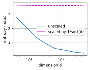
def attention_stats(d, num_keys=64, num_queries=256, scaled=True, seed=0):
    key_q, key_k = jax.random.split(jax.random.key(seed))
    q = jax.random.normal(key_q, (num_queries, d))
    keys = jax.random.normal(key_k, (num_queries, num_keys, d))
    scores = (keys @ q[..., None]).squeeze(-1)
    if scaled:
        scores = scores / math.sqrt(d)
    alpha = jax.nn.softmax(scores, axis=-1)
    entropy = -(alpha * jnp.log(alpha + 1e-12)).sum(-1).mean()
    # Frobenius norm of the softmax Jacobian diag(alpha) - alpha alpha^T
    jac = (alpha[..., None] * jnp.eye(num_keys)
           - alpha[..., :, None] * alpha[..., None, :])
    return float(entropy), float(jnp.sqrt((jac**2).sum((-2, -1))).mean())

ds = [2**k for k in range(2, 10)]
entropies = [[attention_stats(d, scaled=s)[0] for d in ds]
             for s in (False, True)]
d2l.plot(ds, entropies, 'dimension d', 'entropy (nats)',
         legend=['unscaled', 'scaled by 1/sqrt(d)'], xscale='log')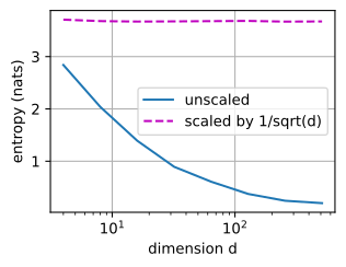
A uniform distribution over \(64\) keys has entropy \(\ln 64 \approx 4.2\) nats. The scaled scores retain an entropy of about \(3.7\) nats across two orders of magnitude in \(d\). Thus the weight distribution retains similar sharpness as the vector dimension grows. Without scaling, the entropy collapses as \(d\) grows—below \(0.2\) nats by \(d = 512\), a near-deterministic weighting that concentrates almost all its mass on a single key purely because the vectors are long. The Jacobian norm measures the corresponding change in the score gradient:
torch.manual_seed(0)
for d in (4, 64, 512):
    _, jac_unscaled = attention_stats(d, scaled=False)
    _, jac_scaled = attention_stats(d, scaled=True)
    print(f'd = {d:3d}: Jacobian norm {jac_unscaled:.3f} (unscaled), '
          f'{jac_scaled:.3f} (scaled)')
d = 4: Jacobian norm 0.259 (unscaled), 0.178 (scaled)
d = 64: Jacobian norm 0.208 (unscaled), 0.182 (scaled)
d = 512: Jacobian norm 0.093 (unscaled), 0.184 (scaled)for d in (4, 64, 512):
_, jac_unscaled = attention_stats(d, scaled=False)
_, jac_scaled = attention_stats(d, scaled=True)
print(f'd = {d:3d}: Jacobian norm {jac_unscaled:.3f} (unscaled), '
f'{jac_scaled:.3f} (scaled)')d = 4: Jacobian norm 0.258 (unscaled), 0.178 (scaled)
d = 64: Jacobian norm 0.218 (unscaled), 0.184 (scaled)
d = 512: Jacobian norm 0.103 (unscaled), 0.186 (scaled)With scaling, the Jacobian norm is the same at every dimension. Without it, the norm decays as the softmax saturates—by \(d = 512\) it has fallen to about half the scaled value and is still shrinking. At realistic dimensions, a model with unscaled scores would therefore begin with near-one-hot attention and small score gradients. Division by \(\sqrt{d}\) removes the dimension-induced scaling, so it is part of the definition Equation 10.2.2 rather than a tuned hyperparameter.
10.2.2 Masking
Attention as defined so far attends to every key. In practice we routinely need it not to, for one of two reasons. The first is padding: sequences of different lengths end up in the same minibatch, padded with dummy tokens to a common length (here shown as <blank>):
Dive  into  Deep    Learning
Learn to    code    <blank>
Hello world <blank> <blank>
Padding tokens carry no meaning, and no query should waste weight on them. The second reason is causality: a language model trained to predict the next token computes outputs for all positions of a sequence in parallel, and the query at position \(t\) must not see keys at positions beyond \(t\)— otherwise the model can copy the very future it is being trained to predict. Both cases call for the same operation: restrict the attention sum \(\sum_{i=1}^n \alpha(\mathbf{q}, \mathbf{k}_i) \mathbf{v}_i\) to a valid prefix \(\sum_{i=1}^l \alpha(\mathbf{q}, \mathbf{k}_i) \mathbf{v}_i\) with \(l \leq n\), where \(l\) depends on the sequence (padding) or on the query position (causality).
10.2.2.1 The Masked Softmax Operation
The masked softmax implements this restriction without branching over keys. It overwrites invalid scores with a very negative number before the softmax, making their normalized weights zero. This formulation preserves the regular array operations used by optimized batched kernels.
The replacement value depends on the numerical precision. Older codebases used a literal constant such as \(-10^{6}\). In single precision that works; in the half precisions that modern training runs in, it does not. The float16 format tops out near \(6.5 \times 10^4\), so \(-10^6\) silently overflows, and in bfloat16 a merely-large constant may fail to fully suppress a weight once genuine scores are large themselves. Writing literal \(-\infty\) masks exactly, but if every key of some query is masked, the softmax returns NaN and can invalidate the training run. We therefore adopt the dtype-safe idiom, which masks with the most negative finite value of the score’s dtype (torch.finfo(X.dtype).min and jnp.finfo(X.dtype).min, respectively): the masked weights are exactly zero at any precision, with no NaN. A fully masked query, which has no valid key, would otherwise produce a uniform average over invalid values. The masked_softmax implementation therefore zeroes such a row, although callers should still ensure that every query retains at least one valid key.
def masked_softmax(X, valid_lens):
    """Perform softmax operation by masking elements on the last axis."""
    # X: 3D tensor, valid_lens: 1D or 2D tensor
    if valid_lens is None:
        return F.softmax(X, dim=-1)
    shape = X.shape
    if valid_lens.dim() == 1:
        valid_lens = torch.repeat_interleave(valid_lens, shape[1])
    else:
        valid_lens = valid_lens.reshape(-1)
    mask = torch.arange(shape[-1], device=X.device)[None, :]
    mask = mask < valid_lens[:, None]
    # Most negative finite score: exactly zero weight after the softmax,
    # at any precision, without the NaN risk of literal -inf
    X = X.reshape(-1, shape[-1]).masked_fill(~mask, torch.finfo(X.dtype).min)
    weights = F.softmax(X, dim=-1)
    # A fully masked query (no valid key) would be a uniform average over
    # invalid values; zero those rows so no padded position leaks through
    weights = torch.where(mask.any(-1, keepdim=True), weights, 0.0)
    return weights.reshape(shape)
def masked_softmax(X, valid_lens):
"""Perform softmax operation by masking elements on the last axis."""
# X: 3D tensor, valid_lens: 1D or 2D tensor
if valid_lens is None:
return jax.nn.softmax(X, axis=-1)
shape = X.shape
if valid_lens.ndim == 1:
valid_lens = jnp.repeat(valid_lens, shape[1])
else:
valid_lens = valid_lens.reshape(-1)
mask = jnp.arange(shape[-1])[None, :] < valid_lens[:, None]
# Most negative finite score: exactly zero weight after the softmax,
# at any precision, without the NaN risk of literal -inf
X = jnp.where(mask, X.reshape(-1, shape[-1]), jnp.finfo(X.dtype).min)
weights = jax.nn.softmax(X, axis=-1)
# A fully masked query (no valid key) would be a uniform average over
# invalid values; zero those rows so no padded position leaks through
weights = jnp.where(mask.any(-1, keepdims=True), weights, 0.0)
return weights.reshape(shape)To illustrate how this function works, consider a minibatch of two examples with two queries and four keys each, where the valid lengths are \(2\) and \(3\), respectively. All weights beyond the valid length come out as zero, and each row still sums to \(1\):
masked_softmax(torch.rand(2, 2, 4), torch.tensor([2, 3]))tensor([[[0.7005, 0.2995, 0.0000, 0.0000],
[0.5080, 0.4920, 0.0000, 0.0000]],
[[0.2296, 0.3997, 0.3707, 0.0000],
[0.1914, 0.4130, 0.3956, 0.0000]]])masked_softmax(jax.random.uniform(jax.random.key(0), (2, 2, 4)),
jnp.array([2, 3]))Array([[[0.4922724 , 0.5077276 , 0. , 0. ],
[0.5997409 , 0.40025908, 0. , 0. ]],
[[0.3531402 , 0.19856434, 0.4482954 , 0. ],
[0.31042197, 0.2873157 , 0.40226236, 0. ]]], dtype=float32)For finer control we can pass a two-dimensional tensor of valid lengths, one per query:
masked_softmax(torch.rand(2, 2, 4), torch.tensor([[1, 3], [2, 4]]))tensor([[[1.0000, 0.0000, 0.0000, 0.0000],
[0.3538, 0.3878, 0.2584, 0.0000]],
[[0.5266, 0.4734, 0.0000, 0.0000],
[0.2870, 0.2921, 0.2345, 0.1864]]])masked_softmax(jax.random.uniform(jax.random.key(1), (2, 2, 4)),
jnp.array([[1, 3], [2, 4]]))Array([[[1. , 0. , 0. , 0. ],
[0.35672572, 0.2543091 , 0.38896522, 0. ]],
[[0.43679553, 0.5632045 , 0. , 0. ],
[0.2580636 , 0.2509437 , 0.258296 , 0.23269679]]], dtype=float32)10.2.2.2 Causal Masking
Per-query valid lengths are exactly what causality needs: for a sequence of length \(n\), the query at position \(t\) may attend to keys \(1, \ldots, t\), so the valid lengths are \((1, 2, \ldots, n)\), shared by every sequence in the batch. The resulting attention pattern is lower triangular:
torch.manual_seed(0)
scores = torch.randn(1, 6, 6)
causal_lens = torch.arange(1, 7)[None, :]  # query t sees keys 1..t
d2l.show_heatmaps(masked_softmax(scores, causal_lens)[None],
                  xlabel='Keys', ylabel='Queries')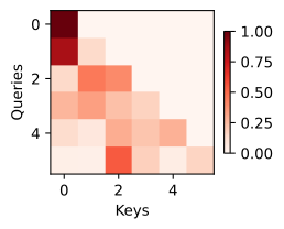
scores = jax.random.normal(jax.random.key(2), (1, 6, 6))
causal_lens = jnp.arange(1, 7)[None, :]  # query t sees keys 1..t
d2l.show_heatmaps(masked_softmax(scores, causal_lens)[None],
                  xlabel='Keys', ylabel='Queries')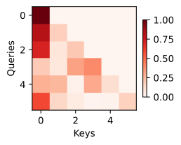
This triangular mask lets a generative model train all sequence positions in parallel without exposing future tokens. Generation additionally requires a shifted next-token objective and a decoding loop. The mask will accompany us through every decoder in the chapters ahead.
10.2.2.3 Composing Masks
valid_lens describes prefixes, which cover the two cases above, but the general interface is a boolean tensor: entry \((i, j)\) says whether query \(i\) may attend to key \(j\). Every requirement takes this form — padding excludes keys beyond the sequence length, causality excludes keys beyond the query, and structural patterns such as the attention windows of Section 10.5 exclude by distance — and a key must survive all requirements at once, so masks compose by logical AND. Broadcasting keeps the bookkeeping cheap: a padding mask has shape \((\textrm{batch}, 1, \textrm{keys})\), a causal mask \((1, \textrm{queries}, \textrm{keys})\), and their AND broadcasts to the full \((\textrm{batch}, \textrm{queries}, \textrm{keys})\) without materializing either input per example. Applying the composite is the same idiom as before: overwrite the excluded scores with the dtype’s most negative finite value, then softmax.
valid_lens, n = torch.tensor([6, 3]), 6
j = torch.arange(n)
padding = (j[None, :] < valid_lens[:, None])[:, None, :]  # (batch, 1, key)
causal = (j[None, :] <= j[:, None])[None, :, :]         # (1, query, key)
mask = padding & causal                                 # (batch, query, key)
torch.manual_seed(0)
scores = torch.randn(2, n, n)
weights = F.softmax(
    scores.masked_fill(~mask, torch.finfo(scores.dtype).min), dim=-1)
d2l.show_heatmaps(weights[:, None], xlabel='Keys', ylabel='Queries')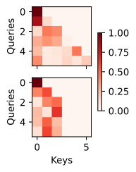
valid_lens, n = jnp.array([6, 3]), 6
j = jnp.arange(n)
padding = (j[None, :] < valid_lens[:, None])[:, None, :]  # (batch, 1, key)
causal = (j[None, :] <= j[:, None])[None, :, :]         # (1, query, key)
mask = padding & causal                                 # (batch, query, key)
scores = jax.random.normal(jax.random.key(0), (2, n, n))
weights = jax.nn.softmax(
    jnp.where(mask, scores, jnp.finfo(scores.dtype).min), axis=-1)
d2l.show_heatmaps(weights[:, None], xlabel='Keys', ylabel='Queries')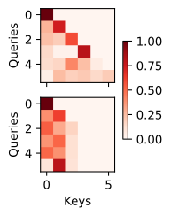
The first sequence shows the plain causal triangle; the second is cut off at its valid length of \(3\), the intersection of both constraints. Composition sharpens the fully-masked hazard flagged above: masks that are harmless alone can leave some query with an empty intersection, so the guarantee of at least one valid key per query must hold for the composite. The same mask composition handles packed sequences, in which several documents are concatenated into one training row. ANDing the causal mask with a block-diagonal mask prevents attention across document boundaries.
10.2.3 Batched Attention
10.2.3.1 Batch Matrix Multiplication
Attention is computed on minibatches of queries, keys, and values, so we need to multiply batches of matrices by one another. Assume that
\[ \mathbf{Q} = [\mathbf{Q}_1, \mathbf{Q}_2, \ldots, \mathbf{Q}_n] \in \mathbb{R}^{n \times a \times b}, \qquad \mathbf{K} = [\mathbf{K}_1, \mathbf{K}_2, \ldots, \mathbf{K}_n] \in \mathbb{R}^{n \times b \times c}. \]
Then the batch matrix multiplication (BMM) computes one matrix product per batch element,
\[\textrm{BMM}(\mathbf{Q}, \mathbf{K}) = [\mathbf{Q}_1 \mathbf{K}_1, \mathbf{Q}_2 \mathbf{K}_2, \ldots, \mathbf{Q}_n \mathbf{K}_n] \in \mathbb{R}^{n \times a \times c}. \tag{10.2.5}\]
A framework batch-matrix multiplication has the expected shape:
Q = torch.ones((2, 3, 4))
K = torch.ones((2, 4, 6))
d2l.check_shape(torch.bmm(Q, K), (2, 3, 6))
Q = jnp.ones((2, 3, 4))
K = jnp.ones((2, 4, 6))
d2l.check_shape(jax.lax.batch_matmul(Q, K), (2, 3, 6))10.2.3.2 The DotProductAttention Class
Scaled dot-product attention can now be written in its matrix form. For \(n\) queries and \(m\) key–value pairs, with queries and keys of length \(d\) and values of length \(v\), stack the queries into \(\mathbf{Q} \in \mathbb{R}^{n \times d}\), the keys into \(\mathbf{K} \in \mathbb{R}^{m \times d}\), and the values into \(\mathbf{V} \in \mathbb{R}^{m \times v}\). Then the entire attention computation is two matrix products and a softmax:
\[ \mathrm{softmax}\left(\frac{\mathbf{Q} \mathbf{K}^\top }{\sqrt{d}}\right) \mathbf{V} \in \mathbb{R}^{n \times v}. \tag{10.2.6}\]
Requiring queries and keys to share the length \(d\) is no real restriction: a learned matrix \(\mathbf{M}\) turns \(\mathbf{q}^\top \mathbf{k}\) into \(\mathbf{q}^\top \mathbf{M} \mathbf{k}\) and translates between spaces of different dimension (an exercise below). Applied to a minibatch, Equation 10.2.6 uses the batch matrix multiplication of Equation 10.2.5 twice. The implementation applies dropout to the attention weights as regularization, and stores the weights for visualization:
class DotProductAttention(nn.Module):
    """Scaled dot product attention."""
    def __init__(self, dropout):
        super().__init__()
        self.dropout = nn.Dropout(dropout)

    # Shape of queries: (batch_size, no. of queries, d)
    # Shape of keys: (batch_size, no. of key-value pairs, d)
    # Shape of values: (batch_size, no. of key-value pairs, value dimension)
    # Shape of valid_lens: (batch_size,) or (batch_size, no. of queries)
    def forward(self, queries, keys, values, valid_lens=None):
        d = queries.shape[-1]
        # Swap the last two dimensions of keys with keys.transpose(1, 2)
        scores = torch.bmm(queries, keys.transpose(1, 2)) / math.sqrt(d)
        self.attention_weights = masked_softmax(scores, valid_lens)
        return torch.bmm(self.dropout(self.attention_weights), values)
class DotProductAttention(nnx.Module):
"""Scaled dot product attention."""
def __init__(self, dropout, rngs=None):
rngs = nnx.Rngs(dropout=0) if rngs is None else rngs
self.dropout = nnx.Dropout(dropout, rngs=rngs)
# Shape of queries: (batch_size, no. of queries, d)
# Shape of keys: (batch_size, no. of key-value pairs, d)
# Shape of values: (batch_size, no. of key-value pairs, value dimension)
# Shape of valid_lens: (batch_size,) or (batch_size, no. of queries)
def __call__(self, queries, keys, values, valid_lens=None):
d = queries.shape[-1]
# Swap the last two dimensions of keys with keys.swapaxes(1, 2)
scores = queries@(keys.swapaxes(1, 2)) / math.sqrt(d)
attention_weights = masked_softmax(scores, valid_lens)
# NNX idiom: return (output, weights); PyTorch stores weights on self
return self.dropout(attention_weights) @ values, attention_weightsTo see the class at work we use a minibatch of size \(2\), with \(10\) keys and values of dimension \(4\), a single \(2\)-dimensional query per example, and valid lengths of \(2\) and \(6\). The output is one \(4\)-dimensional row per query:
torch.manual_seed(0)
queries = torch.randn(2, 1, 2)
keys = torch.randn(2, 10, 2)
values = torch.randn(2, 10, 4)
valid_lens = torch.tensor([2, 6])

attention = DotProductAttention(dropout=0.5)
attention.eval()
d2l.check_shape(attention(queries, keys, values, valid_lens), (2, 1, 4))
queries = jax.random.normal(jax.random.key(0), (2, 1, 2))
keys = jax.random.normal(jax.random.key(1), (2, 10, 2))
values = jax.random.normal(jax.random.key(2), (2, 10, 4))
valid_lens = jnp.array([2, 6])
attention = DotProductAttention(dropout=0.5)
output, attention_weights = nnx.view(
attention, deterministic=True)(queries, keys, values, valid_lens)
d2l.check_shape(output, (2, 1, 4))The stored attention weights confirm the effect of the mask: weights vanish beyond the second and sixth key, respectively.
d2l.show_heatmaps(attention.attention_weights.reshape((1, 1, 2, 10)),
                  xlabel='Keys', ylabel='Queries')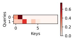
d2l.show_heatmaps(attention_weights.reshape((1, 1, 2, 10)),
                  xlabel='Keys', ylabel='Queries')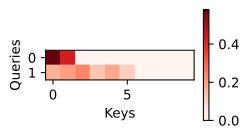
10.2.4 Attention as Learned Alignment
Learned attention first became prominent in neural machine translation. Around 2014, the leading neural approach encoded a source sentence with an RNN into a single fixed-size state vector and decoded the translation from that vector with a second RNN (we build such encoder–decoder models in full in Section 18.1). The design has the flaw this chapter opened with: one fixed-size vector must represent the entire sentence, which becomes increasingly restrictive as sentences grow. Translation quality degraded visibly with sentence length. Graves (2013) had faced a version of this problem when generating handwriting from text, and solved it with a differentiable model that aligned each output pen stroke with a position in the source text—though with the constraint that the alignment could only move forward, an assumption borrowed from decoding in speech recognition (Rabiner and Juang 1993).
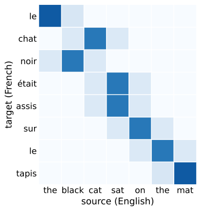
Bahdanau et al. (2015) removed the constraint. Their translation model kept the two RNNs but changed the decoder input at every step. The current decoder state served as a query against all encoder states, which serve as keys and values, and feed the resulting weighted summary—a fresh one per output token—into the next prediction. The paper’s title called the idea “jointly learning to align and translate”, and the learned weights behaved exactly like the soft alignments of classical statistical translation: mostly monotone along the diagonal, with clean departures where the two languages order words differently, as sketched in Figure 10.2.1. The training objective did not directly supervise these alignments; they emerged while the model learned translation. This computation instantiates the attention mechanism in Equation 10.1.1.
One detail differed from the scoring function we settled on above. The decoder state and the encoder states were vectors of different sizes, so instead of a dot product, Bahdanau et al. (2015) scored with a small one-hidden-layer MLP, now known as additive attention:
\[a(\mathbf{q}, \mathbf{k}) = \mathbf{w}_v^\top \tanh(\mathbf{W}_q \mathbf{q} + \mathbf{W}_k \mathbf{k}) \in \mathbb{R}, \tag{10.2.7}\]
where \(\mathbf{W}_q \in \mathbb{R}^{h \times q}\), \(\mathbf{W}_k \in \mathbb{R}^{h \times k}\), and \(\mathbf{w}_v \in \mathbb{R}^{h}\) are learned. The two projections embed queries and keys into a shared \(h\)-dimensional space, and \(\mathbf{w}_v\) reads a score off the sum. It takes only a few lines to compute—here scoring three \(20\)-dimensional queries against six \(2\)-dimensional keys, dimensions no dot product could pair up:
torch.manual_seed(0)
queries, keys = torch.randn(3, 20), torch.randn(6, 2)
num_hiddens = 8
W_q = torch.randn(num_hiddens, 20) / math.sqrt(20)
W_k = torch.randn(num_hiddens, 2) / math.sqrt(2)
w_v = torch.randn(num_hiddens) / math.sqrt(num_hiddens)
features = torch.tanh((queries @ W_q.T)[:, None, :]
                      + (keys @ W_k.T)[None, :, :])
scores = features @ w_v
d2l.check_shape(scores, (3, 6))
F.softmax(scores, dim=-1)
tensor([[0.1692, 0.1612, 0.1816, 0.1560, 0.1502, 0.1818],
[0.1664, 0.1849, 0.1657, 0.1338, 0.1623, 0.1870],
[0.1517, 0.2188, 0.1441, 0.1317, 0.2166, 0.1371]])key_q, key_k, k1, k2, k3 = jax.random.split(jax.random.key(0), 5)
queries = jax.random.normal(key_q, (3, 20))
keys = jax.random.normal(key_k, (6, 2))
num_hiddens = 8
W_q = jax.random.normal(k1, (num_hiddens, 20)) / math.sqrt(20)
W_k = jax.random.normal(k2, (num_hiddens, 2)) / math.sqrt(2)
w_v = jax.random.normal(k3, (num_hiddens,)) / math.sqrt(num_hiddens)
features = jnp.tanh((queries @ W_q.T)[:, None, :]
+ (keys @ W_k.T)[None, :, :])
scores = features @ w_v
d2l.check_shape(scores, (3, 6))
jax.nn.softmax(scores, axis=-1)Array([[0.13390937, 0.3772766 , 0.17127123, 0.1027277 , 0.06276076,
0.15205443],
[0.19218282, 0.31524566, 0.14511336, 0.08953383, 0.07662669,
0.18129766],
[0.15669951, 0.3378386 , 0.15281527, 0.11713327, 0.09428051,
0.1412329 ]], dtype=float32)Dot-product attention later became the standard choice partly because it maps efficiently to accelerator hardware. All query–key dot products form one matrix multiplication, whereas the additive score requires an \(n \times m \times h\) tensor of hidden activations. When a learned metric is wanted, we can project queries and keys with learned matrices before the dot product and have it at matmul speed—which is precisely the form attention takes inside the Transformer, whose authors then discarded the RNN scaffolding altogether and kept attention as the only mechanism relating sequence positions (Vaswani et al. 2017). The next next sections develop multiple attention heads and then introduce explicit positional information to replace the RNN’s sequential ordering.
10.2.5 Summary
Scaled dot-product attention computes scores with one batched matrix multiplication. Dividing by \(\sqrt d\) keeps the score variance independent of dimension and prevents premature softmax saturation. A mask excludes padding, future positions, or other invalid query–key pairs before normalization; use the most negative finite value of the dtype so the operation remains valid in reduced precision. Boolean masks for several constraints compose by logical AND. DotProductAttention combines scoring, masking, dropout, and value pooling. Additive attention provides an alternative learned score and was the form used in the original neural alignment model.
10.2.6 Exercises
- Invariances of the score. The Gaussian score Equation 10.2.1 and the scaled dot product Equation 10.2.2 both define attention weights through the softmax Equation 10.2.3.
- For each of the two scores, determine which of the following transformations leaves the weights unchanged: adding one vector \(\mathbf{c}\) to every key; adding \(\mathbf{c}\) to the query and to every key; multiplying the query and every key by one orthogonal matrix.
- Queries and keys are usually computed from inputs by affine maps, \(\mathbf{q} = \mathbf{W}_q \mathbf{x} + \mathbf{b}_q\) and \(\mathbf{k}_i = \mathbf{W}_k \mathbf{y}_i + \mathbf{b}_k\). Expand \(\mathbf{q}^\top \mathbf{k}_i\) into four terms and show that the weights do not depend on \(\mathbf{b}_k\). What is the gradient of the loss with respect to \(\mathbf{b}_k\)?
- Through which of the four terms does \(\mathbf{b}_q\) affect the weights, and what preference over the keys can it express that the bias-free score cannot?
- [code] Distance-based attention. Equation Equation 10.2.1 writes the Gaussian score as a dot product minus two squared norms, and the section drops the key-norm term to arrive at Equation 10.2.2.
- Modify
DotProductAttentionso that it keeps the term \(-\tfrac{1}{2}\|\mathbf{k}_i\|^2\), using one batch matrix multiplication for the dot products and a broadcast of the \(m\) squared key norms, without forming the \(n \times m \times d\) tensor of differences \(\mathbf{q} - \mathbf{k}_i\). Apply the \(1/\sqrt{d}\) scaling to both terms. - Verify on random inputs that the resulting weights equal those of a direct evaluation of \(\exp(-\|\mathbf{q} - \mathbf{k}_i\|^2 / (2\sqrt{d}))\) normalized over the keys.
- Compare the weights of the two scoring rules on the inputs of Section 10.2.3.2, ten random two-dimensional keys per example. For which keys do the rules disagree most, and why?
- Modify
- Entropy of random scores. ● The scaled curve of
attention_statsstays near \(3.7\) nats, below the uniform value \(\ln 64 \approx 4.16\). Fix one query \(\mathbf{q} \in \mathbb{R}^d\) and draw \(m\) keys with independent standard normal coordinates, asattention_statsdoes.- Show that the scaled scores \(a_i = \mathbf{q}^\top \mathbf{k}_i /
\sqrt{d}\) are independent normal variables with mean \(0\) and variance \(s^2 = \|\mathbf{q}\|^2 / d\), and compute the expected value of \(s^2\) when \(\mathbf{q}\) is drawn as in
attention_stats. - The entropy of the weights is \(H = \ln Z - \sum_i \alpha_i a_i\) with \(Z = \sum_j \exp(a_j)\). For large \(m\), replace \(Z/m\) and \(\sum_i \exp(a_i)\, a_i / m\) by their expected values and derive \[H \approx \ln m - \frac{s^2}{2}.\] Evaluate the approximation for \(m = 64\) and \(s = 1\).
- The approximation needs \(Z\) to concentrate around its mean. Compute the relative standard deviation of \(Z\) as a function of \(s\) and \(m\), and derive from it a condition on \(s^2\) under which the approximation holds. Unscaled scores have \(s^2 = \|\mathbf{q}\|^2\), whose expected value is \(d\). Evaluate the relative standard deviation for \(m = 64\) at \(s^2 = 4\) and \(s^2 = 8\), and compare the approximation with the unscaled entropies that
attention_statsreturns for \(d = 4\) and \(d = 8\).
- Show that the scaled scores \(a_i = \mathbf{q}^\top \mathbf{k}_i /
\sqrt{d}\) are independent normal variables with mean \(0\) and variance \(s^2 = \|\mathbf{q}\|^2 / d\), and compute the expected value of \(s^2\) when \(\mathbf{q}\) is drawn as in
- [code] The softmax Jacobian.
attention_statsmeasures the Frobenius norm of the Jacobian Equation 10.2.4.- Derive Equation 10.2.4 from Equation 10.2.3, show that for finite scores its null space is spanned by the all-ones vector, and check the formula against automatic differentiation on a random score vector.
- Compute the Frobenius norm when \(\boldsymbol{\alpha}\) is one-hot and when it is uniform over \(m\) keys, and evaluate the uniform case for \(m = 64\). Show that the squared norm is close to \(\sum_i \alpha_i^2\) when every weight is small, and use this to explain why the scaled norms printed for \(d \in \{4, 64, 512\}\) exceed the uniform value.
- Compute the norm for weights spread uniformly over \(k\) of the \(m\) keys, find the \(k\) that maximizes it, and confirm by sampling random weight vectors that none exceeds this maximum. Use the result to explain why the unscaled norm printed for \(d = 4\) exceeds the scaled one.
- Fully masked rows.
masked_softmaxoverwrites excluded scores with the most negative finite value of the dtype and then zeroes the rows of queries that have no valid key.- Explain why, without the final zeroing, a fully masked row returns the uniform distribution, and why the same row returns NaN when the scores are overwritten with \(-\infty\) instead. Trace both cases through the subtraction of the row maximum that a numerically stable softmax performs.
- An older codebase overwrites excluded scores with the constant \(-10^6\) and computes its scores in float16, whose largest finite magnitude is about \(6.55 \times 10^4\). Determine the value that the constant takes when it is rounded to float16, and state what the softmax of such a codebase returns for a fully masked row and for a row with at least one valid key.
- In a self-attention layer, whose queries, keys, and values all come from the same sequence, let a query at a padding position have no valid key, as the composite masks of Section 10.2.2.3 can arrange, and let the excluded scores be overwritten with \(-\infty\), so that the output at that position is NaN. That output is discarded, and in the next attention layer every valid query excludes the padding position as a key. Explain why the NaN nevertheless corrupts the outputs of all valid positions of that sequence in the next layer.
- Composite masks. Section 10.2.2.3 combines masks by logical AND and warns that masks that are harmless alone can leave a query with no valid key. A causal sliding window of width \(w\) lets the query at position \(t\) attend to the keys at positions \(t - w + 1, \ldots,
t\).
- For a sequence of length \(6\) with valid length \(3\), write the padding mask and the causal sliding window of width \(2\) as \(6 \times 6\) boolean matrices. Check that each leaves every query at least one key, and find the queries whose row of the AND is empty.
- Show that an AND of masks has no empty row if every mask allows each query to attend to its own position. Which of the padding, causal, sliding-window, and packed-sequence masks satisfy this condition, and what does the answer say about the empty rows you found?
- Some implementations add a bias matrix with entries \(0\) for allowed pairs and \(c < 0\) for excluded pairs, and compose masks by adding their biases. Take for \(c\) the most negative finite single-precision value, about \(-3.4 \times 10^{38}\). Compute the sum of two such biases in single precision, and determine what the softmax returns for a row in which every key is excluded by both masks and for a row in which every key is excluded but some keys by only one mask.
- [code] Two masking conventions.
masked_softmaxdescribes the valid keys of a query by a prefix length, whereas the masks of Section 10.2.2.3 and many libraries use a boolean tensor in whichTruemarks a pair the query may attend to.- Write a converter from
valid_lensof shape (batch size,) or (batch size, number of queries) to a boolean mask of shape (batch size, number of queries, number of keys), and a variant ofmasked_softmaxthat takes such a mask. - Verify on ten random padding and causal configurations that both routes produce identical weights, including for fully masked rows.
- Pack two documents of lengths \(4\) and \(2\) into one row of length \(6\). Build the boolean mask that combines the causal mask with the block-diagonal mask of document indices, and verify that attention with your variant gives each document the outputs it receives when it is processed alone with a causal mask.
- Which of the following masks can be expressed by one prefix length per query: padding, causal, padding combined with causal, the packed mask, and a causal sliding window? State what the boolean interface costs in memory for \(B\) sequences of length \(n\) relative to
valid_lens.
- Write a converter from
- [code] Attention dropout.
DotProductAttentionapplies dropout with rate \(p\) to the attention weights, and the weights it exposes for visualization are those before dropout. Dropout multiplies each kept weight by \(1/(1 - p)\) and sets the others to zero, so a row of weights no longer sums to \(1\).- Show that the row sum after dropout has expectation \(1\) and variance \(\frac{p}{1-p} \sum_i \alpha_i^2\), and evaluate the variance for a row that is uniform over \(l\) keys and for a one-hot row. What is the output of a one-hot row in the draws in which dropout removes the attended weight?
- Use the inputs of Section 10.2.3.2 with dropout \(0.5\) active, and pass as values a batch of \(10 \times 10\) identity matrices, so that each output row equals the weights after dropout. Compare the mean and the variance of the row sums over many draws with the prediction computed from the weights before dropout.
- [code] Keys of a different width. Section 10.2.3.2 notes that a matrix \(\mathbf{M} \in \mathbb{R}^{d_q \times d_k}\) turns the dot product into the score \(\mathbf{q}^\top \mathbf{M} \mathbf{k}\) for queries \(\mathbf{q} \in \mathbb{R}^{d_q}\) and keys \(\mathbf{k} \in
\mathbb{R}^{d_k}\).
- Implement this score for a batch of \(n\) queries and \(m\) keys with a learnable \(\mathbf{M}\), and test it on three \(20\)-dimensional queries against six \(2\)-dimensional keys, the dimensions used in Section 10.2.4. Count the floating-point operations of the two evaluation orders \((\mathbf{Q}\mathbf{M})\mathbf{K}^\top\) and \(\mathbf{Q}(\mathbf{M}\mathbf{K}^\top)\) for these dimensions, and state the rule that decides between them.
- The factorization \(\mathbf{M} = \mathbf{W}_q^\top \mathbf{W}_k\) with \(\mathbf{W}_q \in \mathbb{R}^{r \times d_q}\) and \(\mathbf{W}_k \in \mathbb{R}^{r \times d_k}\) turns the score into a dot product of two projected vectors. Count the parameters of both parameterizations, find the values of \(r\) for which the factored form has fewer, and state the constraint it places on \(\mathbf{M}\).
- Let \(\mathbf{q}\) and \(\mathbf{k}\) have independent zero-mean, unit-variance coordinates, and let \(\mathbf{W}_q\) and \(\mathbf{W}_k\) have independent zero-mean entries of variance \(1/d_q\) and \(1/d_k\), as
W_qandW_kin Section 10.2.4 do. Compute the variance of the factored score, and state the factor that replaces \(1/\sqrt{d}\).
- Arithmetic intensity of attention. For \(n\) queries and \(m\) keys, with queries and keys of width \(d\) and values of width \(v\), the two matrix products of Equation 10.2.6 cost \(2nmd\) and \(2nmv\) floating-point operations, and the softmax costs a few operations per score.
- Suppose that the score matrix is written to memory once and read once by the softmax, whose output is written once and read once by the value product, all in single precision. Count the bytes moved by these four passes, and by reading \(\mathbf{Q}\), \(\mathbf{K}\), \(\mathbf{V}\) and writing the output.
- Neglecting the softmax arithmetic, form the ratio of operations to bytes and let \(n, m \to \infty\) at fixed \(d\) and \(v\). Show that the limit is \((d + v)/8\), and state how the softmax arithmetic changes it.
- Look up the peak arithmetic throughput and the memory bandwidth of one accelerator, compute its ratio of operations per byte, and decide whether attention with \(d = v = 64\) is limited by arithmetic or by memory traffic on it.
- [code] Additive scores near zero. ● The additive score Equation 10.2.7 adds the projected query and the projected key inside a \(\tanh\).
- Replace \(\tanh\) by the identity and show that the attention weights then do not depend on the query.
- Expand \(\tanh\) to third order around zero, identify the lowest-order terms through which the weights depend on the query, and state how this dependence scales when \(\mathbf{W}_q\) and \(\mathbf{W}_k\) are both multiplied by a small factor \(\epsilon\).
- Multiply
W_qandW_kin the code of Section 10.2.4 by \(\epsilon \in \{1, 0.3, 0.1, 0.03\}\), and measure the largest difference between the weight rows of the three queries. Check the scaling you derived, and state what the result for \(\epsilon = 1\) implies for additive attention at initialization.
- [code] Additive versus dot-product cost. ● Score \(n\) queries of width \(d_q\) against \(m\) keys of width \(d_k\) with the additive rule Equation 10.2.7 of hidden size \(h\), and \(n\) queries against \(m\) keys of a shared width \(d\) with Equation 10.2.2.
- Count the parameters, the floating-point operations, and the size of the largest intermediate tensor for each rule.
- Implement a batched version of Equation 10.2.7 that produces weights of shape (batch size, \(n\), \(m\)), and check it against the unbatched code of Section 10.2.4.
- Time both rules for a batch of \(4\) sequences with \(n = m = 512\) at \(d_q = d_k = d = h = 64\) and at \(d_q = d_k = d = h = 256\). Relate the ratio of the two times to your counts of operations and of intermediate memory.
- [extended] A learned alignment. ● Bahdanau et al. (2015) observed that attention weights trained only for translation behave like alignments (Figure 10.2.1). The same effect appears in a toy model without recurrent networks. Draw source sequences of \(8\) tokens uniformly from a vocabulary of \(16\), and let the target at output position \(j\) be the source token at position \(\pi(j)\) for a fixed permutation \(\pi\) of the positions. Score one learned query per output position against keys that a learned linear map computes from the concatenated one-hot token and one-hot position of each source token, use the one-hot source tokens as values, and train on the negative logarithm of the output entry that belongs to the target token.
- Implement the model with
DotProductAttention, train it, and plot the attention weights of one sequence withd2l.show_heatmaps. Compare the map with \(\pi\). - Replace the score by the additive rule Equation 10.2.7 and compare the number of steps that each model needs to reach \(99\%\) accuracy.
- Give queries and keys the width \(d \in \{16, 256, 1024\}\) with standard normal initialization, and train with and without the factor \(1/\sqrt{d}\). Relate the training curves to the entropy of the weights at initialization.
- Explain why a fixed query per output position cannot learn a reordering that depends on the tokens, such as swapping two neighbors only when the first belongs to a designated subset of the vocabulary, and state what the query would have to depend on.
- Implement the model with