%matplotlib inline
from d2l import torch as d2l
import numpy as np
import torch27.2 Distributions
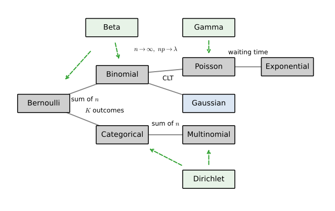
A distribution assigns probabilities to the possible values of a random variable (Section 27.1). This section develops eleven data distributions and three conjugate priors used frequently in machine learning and relates them through constructions and limits. A sum of Bernoulli variables has a binomial distribution. Appropriate many-trial limits yield the Poisson or, under the central limit theorem, the Gaussian distribution. The categorical distribution extends Bernoulli variables to \(K\) outcomes and provides the probabilistic model behind a softmax classifier. Many of these distributions belong to the exponential family and admit conjugate priors, which simplifies maximum-likelihood and Bayesian calculations.
Figure 27.2.1 summarizes these relationships. Its arrows denote constructions and limiting arguments, and the enclosing region marks the distributions that belong to the exponential family.
The first two parts form a reference gallery; the exponential-family and conjugacy parts explain shared structure. A modeling choice also depends on the support and data-generating question:
| observed quantity | useful starting model | condition or omission to check |
|---|---|---|
| binary or one-of-\(K\) outcome | Bernoulli or categorical | probabilities may depend on covariates |
| successes in fixed trials | binomial | conditionally independent trials with a common success probability |
| event count over exposure | Poisson | mean equals variance; overdispersion may require another count law |
| positive waiting time | exponential | constant hazard; Gamma, Weibull, and log-normal laws are omitted |
| bounded continuous value | continuous uniform as a baseline | an application need not have constant density |
| real-valued residual | Gaussian or Laplace | mixtures and heavier-tailed laws may fit better |
| correlated real vector | multivariate Gaussian | multimodality and structured covariance need richer models |
For each distribution we use a common template: its mass or density function, where it arises in machine learning, its mean and variance derived rather than asserted, and a compact teaching cell that evaluates the law and draws a sample. We treat the discrete distributions first, then the continuous ones, then unify them, using the following imports throughout.
%matplotlib inline
from d2l import tensorflow as d2l
import numpy as np
import tensorflow as tf%matplotlib inline
from d2l import jax as d2l
import numpy as np
import jax
from jax import numpy as jnp%matplotlib inline
from d2l import mxnet as d2l
import numpy as npThis section works in plain NumPy: every computation here is elementary array arithmetic, so nothing beyond NumPy is needed.
27.2.1 Discrete Distributions
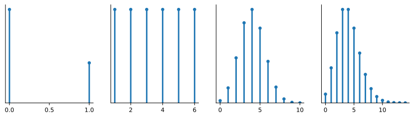
A discrete random variable takes values in a countable set, and its distribution is a probability mass function (pmf) \(p_k = P(X=k)\) with \(p_k\ge0\) and \(\sum_k p_k=1\). Mean and variance are the sums \(\mathbb E[X]=\sum_k k\,p_k\) and \(\operatorname{Var}(X)=\mathbb E[X^2]-\mathbb E[X]^2\) (Section 27.1). The five distributions here form a connected chain: each is built from, or is a limit of, the one before. Figure 27.2.2 shows their shapes side by side so the shared bell-like silhouette of the count distributions is visible at a glance.
27.2.1.1 Bernoulli
The Bernoulli is the simplest non-trivial random variable: a single coin flip that comes up \(1\) with probability \(p\) and \(0\) with probability \(1-p\). We write \(X\sim\mathrm{Bernoulli}(p)\), with pmf
\[ p_1 = P(X=1) = p, \qquad p_0 = P(X=0) = 1-p . \tag{27.2.1}\]
Where it arises. A probabilistic binary classifier commonly uses a Bernoulli output: the model emits \(\hat p\), and the negative log-likelihood \(-y\log\hat p-(1-y)\log(1-\hat p)\) is exactly the binary cross-entropy loss, the maximum-likelihood view of binary classification developed in Section 27.3.2.1.
Mean and variance. Because \(X\) takes only the values \(0\) and \(1\), we have \(X^2=X\), which makes both moments immediate:
\[ \mu_X = \mathbb E[X] = 1\cdot p + 0\cdot(1-p) = p, \qquad \sigma_X^2 = \mathbb E[X^2]-\mu_X^2 = p - p^2 = p(1-p). \]
The variance \(p(1-p)\) is largest at \(p=\tfrac12\) (the fairest, least predictable coin) and vanishes at \(p\in\{0,1\}\) (a certain outcome carries no randomness).
import numpy as onp
rng = onp.random.default_rng(0)
p = 0.3
sample = 1 * (rng.random((3, 3)) < p)          # 1 with prob p, else 0
big = 1 * (rng.random(10000) < p)              # large sample for the mean
print('pmf  P(0), P(1) =', (1 - p, p))
print('mean of 10,000 draws =', float(big.mean()), ' (≈ p)')
sample
pmf P(0), P(1) = (0.7, 0.3)
mean of 10,000 draws = 0.3006 (≈ p)array([[0, 1, 1],
[1, 0, 0],
[0, 0, 0]])27.2.1.2 Categorical and Multinomial
The categorical distribution generalizes the Bernoulli from two outcomes to \(K\). It is parameterized by a probability vector \(\mathbf p=(p_1,\dots,p_K)\) with \(p_k\ge0\) and \(\sum_k p_k=1\), and a draw lands on class \(k\) with probability \(p_k\),
\[ P(X=k) = p_k . \tag{27.2.2}\]
Where it arises. Every softmax output layer turns a vector of scores (logits) \(\mathbf z\) into a categorical over classes or vocabulary tokens via
\[ p_k = \frac{e^{z_k}}{\sum_{j=1}^{K} e^{z_j}}, \tag{27.2.3}\]
and the negative log-likelihood of the categorical, \(-\sum_k y_k\log p_k\) with \(\mathbf y\) the one-hot label, is exactly the softmax cross-entropy loss (Section 27.3.2.1, Section 3.1). The Bernoulli is the case \(K=2\). To sample a class rather than score one, the Gumbel-max trick perturbs each logit with independent Gumbel noise (the Gumbel distribution is the location–scale law of the maxima of many independent draws (Gumbel 1954)) and takes the argmax: an exact categorical sampler, and the basis of the Gumbel-softmax relaxation that lets gradients flow through discrete choices (Jang et al. 2017; Maddison et al. 2017).
The multinomial is its count version, the categorical analogue of how the binomial sums Bernoullis. Drawing \(n\) independent categorical samples and counting how often each class occurs gives a vector \(\mathbf x=(x_1,\dots,x_K)\) with \(\sum_k x_k=n\) and pmf
\[ P(\mathbf x) = \frac{n!}{x_1!\cdots x_K!}\,\prod_{k=1}^{K} p_k^{x_k}, \tag{27.2.4}\]
the multinomial coefficient counting the orderings that yield those counts, times the probability \(\prod_k p_k^{x_k}\) of any one such ordering. For \(K=2\) this is the binomial of the next section.
The teaching cell turns a logit vector into a categorical via softmax, confirms it normalizes, and draws one sample.
import numpy as onp
rng = onp.random.default_rng(0)
z = onp.array([2.0, 1.0, 0.1, -1.0])            # logits over K = 4 classes
p_cat = onp.exp(z) / onp.exp(z).sum()            # softmax -> categorical
draw = int(rng.choice(len(p_cat), p=p_cat))
print('categorical p =', p_cat.round(3), ' sum =', float(p_cat.sum()))
print('one sample -> class', draw)
categorical p = [0.638 0.235 0.095 0.032] sum = 1.0
one sample -> class 027.2.1.3 Discrete Uniform
If a categorical assigns equal probability to each of its outcomes it is the discrete uniform. Supported on \(\{1,2,\dots,n\}\), every value is equally likely, \(p_i=\tfrac1n\), written \(X\sim U(n)\).
Where it arises. It models a fair die, a uniformly chosen index, or a token sampled with no preference. It is also the maximum-entropy distribution on a finite set, a fact we take as given (Cover and Thomas 1999) and place in context when we meet the exponential family below.
Mean and variance. Both follow from the closed forms \(\sum_{i=1}^n i=\tfrac{n(n+1)}2\) and \(\sum_{i=1}^n i^2=\tfrac{n(n+1)(2n+1)}6\):
\[ \mu_X = \frac1n\sum_{i=1}^n i = \frac{n+1}{2}, \qquad \sigma_X^2 = \frac1n\sum_{i=1}^n i^2 - \mu_X^2 = \frac{n^2-1}{12}. \]
The mean is the midpoint, by symmetry; the variance grows like \(n^2\), since a wider range of equally likely values is more spread out. The cell checks both formulas against a large sample of die rolls.
rng = np.random.default_rng(0)
n = 6
sample = rng.integers(1, n + 1, 10000)           # 10,000 die rolls
print('mean (n+1)/2  =', (n + 1) / 2, '   sample mean:', float(sample.mean()))
print('var (n^2-1)/12 =', round((n**2 - 1) / 12, 3), ' sample var :',
      float(sample.var().round(3)))
mean (n+1)/2 = 3.5 sample mean: 3.5045
var (n^2-1)/12 = 2.917 sample var : 2.93727.2.1.4 Binomial
Sum \(n\) independent Bernoulli flips and you count successes: this is the binomial. Writing each flip as \(X_i\sim\mathrm{Bernoulli}(p)\) with \(1\) for success,
\[ X = \sum_{i=1}^{n} X_i \sim \mathrm{Binomial}(n,p). \tag{27.2.5}\]
Exactly \(k\) successes can occur in \(\binom nk\) orderings, each of probability \(p^k(1-p)^{n-k}\), so
\[ P(X=k) = \binom{n}{k}\,p^k(1-p)^{n-k}, \qquad k=0,1,\dots,n. \tag{27.2.6}\]
Where it arises. It models any “how many out of \(n\)” count with a fixed per-trial probability: clicks among impressions, correct predictions on a held-out batch, heads in a run of flips.
Mean and variance, via the sum. Rather than wrestle with the binomial coefficient, use the representation Equation 27.2.5 as a sum of Bernoullis. Expectation is linear (always, even for dependent terms), so
\[ \mu_X = \mathbb E\Bigl[\sum_i X_i\Bigr] = \sum_i \mathbb E[X_i] = np . \]
The \(X_i\) are independent, and variance is additive over independent summands, so
\[ \sigma_X^2 = \operatorname{Var}\Bigl(\sum_i X_i\Bigr) = \sum_i \operatorname{Var}(X_i) = np(1-p) . \]
Representing a binomial variable as a sum of Bernoulli variables gives its mean and variance without manipulating binomial coefficients. Successive pmf terms differ by the ratio
\[ \frac{P(X=k+1)}{P(X=k)} = \frac{n-k}{k+1}\cdot\frac{p}{1-p}, \]
so the whole pmf builds up from \(P(X=0)=(1-p)^n\) by repeated multiplication, with never a factorial in sight.
import numpy as onp
rng = onp.random.default_rng(0)
n, p = 10, 0.4
pmf = onp.zeros(n + 1)
pmf[0] = (1 - p)**n
for k in range(n):                               # successive-ratio recursion
    pmf[k + 1] = pmf[k] * (n - k) / (k + 1) * p / (1 - p)
print('mean onp =', n * p, '  var onp(1-p) =', n * p * (1 - p))
print('P(X=k):', pmf.round(3))
rng.binomial(n, p, size=(3, 3))                  # sample counts of successes
mean onp = 4.0 var onp(1-p) = 2.4
P(X=k): [0.006 0.04 0.121 0.215 0.251 0.201 0.111 0.042 0.011 0.002 0. ]array([[5, 3, 1],
[1, 5, 6],
[4, 5, 4]])27.2.1.5 Poisson
What if the trials become many and each rare? Standing at a bus stop, the chance of an arrival in any tiny sub-interval is small, but there are many such intervals. Let \(\lambda\) be the expected number of arrivals per minute. Split the minute into \(n\) slices, model each as \(\mathrm{Bernoulli}(\lambda/n)\), and the count is \(\mathrm{Binomial}(n,\lambda/n)\). Its mean is \(n\cdot\lambda/n=\lambda\) for every \(n\), and its variance \(n\cdot\tfrac{\lambda}{n}(1-\tfrac{\lambda}{n})\to\lambda\). The moments stabilize, which signals that a limiting distribution exists.
The limit, derived. Take \(\mathrm{Binomial}(n,p_n)\) with \(n\to\infty\) and \(p_n\to0\) such that \(np_n\to\lambda\), the law of rare events. Writing \(p_n=\lambda/n\), the pmf at a fixed \(k\) factors into four pieces:
\[ \binom{n}{k}\Bigl(\frac\lambda n\Bigr)^k\Bigl(1-\frac\lambda n\Bigr)^{n-k} = \underbrace{\frac{n!}{(n-k)!\,n^k}}_{\to\,1} \cdot \frac{\lambda^k}{k!} \cdot \underbrace{\Bigl(1-\frac\lambda n\Bigr)^{n}}_{\to\,e^{-\lambda}} \cdot \underbrace{\Bigl(1-\frac\lambda n\Bigr)^{-k}}_{\to\,1} . \]
The first factor is \(\tfrac{n(n-1)\cdots(n-k+1)}{n^k}\to1\), the third is the classic limit \((1-\lambda/n)^n\to e^{-\lambda}\), and the last \(\to1\). Collecting the survivors gives the Poisson pmf:
\[ P(X=k) = \frac{\lambda^k e^{-\lambda}}{k!}, \qquad k=0,1,2,\dots \tag{27.2.7}\]
with \(\lambda>0\) the rate, the average count per unit time; we write \(X\sim\mathrm{Poisson}(\lambda)\).
Where it arises. Counts of rare events with no fixed ceiling: click counts, photons on a sensor, mutations in a genome, requests hitting a server. Run over the whole timeline, the bus-stop slicing above is the Poisson process: the event counts in disjoint time windows are independent Poisson variables.
Mean and variance. The binomial moments suggest the answer, but convergence in distribution alone does not automatically pass unbounded moments to the limit. The Poisson pmf verifies them directly:
\[ E[X]=\sum_{k\ge1}k e^{-\lambda}\frac{\lambda^k}{k!} =\lambda, \qquad E[X(X-1)]=\lambda^2. \]
Therefore
\[ \mu_X=\lambda, \qquad \sigma_X^2=E[X(X-1)]+E[X]-E[X]^2=\lambda. \]
Mean equals variance is the Poisson fingerprint: over-dispersed count data (where the empirical variance exceeds the mean) is the standard sign that a plain Poisson model is too simple. The standard fix, a Poisson whose rate is itself random, reappears later in this section as the Gamma–Poisson mixture, better known as the negative binomial.
import numpy as onp
rng = onp.random.default_rng(0)
lam = 4.0
k = onp.arange(15)
pmf = onp.empty_like(k, dtype=float)
pmf[0] = onp.exp(-lam)
for j in range(len(k) - 1):                    # P(j+1) / P(j) = lambda / (j+1)
    pmf[j + 1] = pmf[j] * lam / (j + 1)
print('mean = var = lambda =', lam)
print('P(X=k):', pmf.round(3))
rng.poisson(lam, size=(3, 3))                   # sample event counts
mean = var = lambda = 4.0
P(X=k): [0.018 0.073 0.147 0.195 0.195 0.156 0.104 0.06 0.03 0.013 0.005 0.002
0.001 0. 0. ]array([[2, 0, 7],
[3, 4, 4],
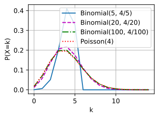
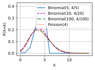
[6, 6, 4]])Watching the limit happen. The limit is visible in a plot. The cell below overlays the pmf of \(\mathrm{Binomial}(n,\lambda/n)\) for growing \(n\) on its \(\mathrm{Poisson}(\lambda)\) limit, building every pmf by the same successive-ratio trick we used for the binomial (for the Poisson the ratio is simply \(P(X=k+1)/P(X=k)=\lambda/(k+1)\)). Already at \(n=20\) the curves are visibly closing in on each other, and at \(n=100\) they coincide to plotting accuracy.
lam, ks = 4.0, np.arange(15)

def binomial_pmf(n, p):                # successive-ratio recursion, no factorials
    pmf = [(1 - p)**n]
    for k in range(len(ks) - 1):
        pmf.append(pmf[-1] * max(n - k, 0) / (k + 1) * p / (1 - p))
    return np.array(pmf)

poisson_pmf = [np.exp(-lam)]
for k in range(len(ks) - 1):
    poisson_pmf.append(poisson_pmf[-1] * lam / (k + 1))
d2l.plot(ks, [binomial_pmf(n, lam / n) for n in (5, 20, 100)]
         + [np.array(poisson_pmf)], xlabel='k', ylabel='P(X=k)',
         legend=[f'Binomial({n}, 4/{n})' for n in (5, 20, 100)] + ['Poisson(4)'])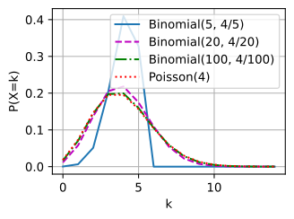
27.2.2 Continuous Distributions
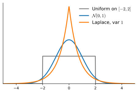
A continuous random variable is described by a probability density (pdf) \(p(x)\ge0\) with \(\int p(x)\,dx=1\); probabilities are areas under it and expectations are integral averages (Section 25.4). The five laws below run from the structureless (uniform) to the universal (Gaussian) to the vector-valued (multivariate Gaussian), with the exponential covering waiting times on \([0,\infty)\) and the Laplace the symmetric case with heavier-than-Gaussian tails. Figure 27.2.3 overlays the three densities on the whole line so their tail behavior is directly comparable: the Gaussian’s thin \(e^{-x^2}\) tail, the Laplace’s heavier \(e^{-|x|}\) tail and sharp peak, and the uniform’s flat plateau.
27.2.2.1 Continuous Uniform
Refine the discrete uniform (let the \(n\) equally likely points fill an interval \([a,b]\)) and you reach the continuous uniform, which picks a value in \([a,b]\) with every value equally likely. The density is constant on the interval and zero outside, with the constant fixed by \(\int p=1\):
\[ p(x) = \begin{cases}\frac{1}{b-a} & x\in[a,b],\\ 0 & \text{otherwise,}\end{cases} \qquad X\sim U(a,b). \tag{27.2.8}\]
Where it arises. It is the raw material of randomness: the \(U(0,1)\) generator underlies inverse-transform sampling (Section 27.1), Monte Carlo, dropout masks, and random weight initialization.
Mean and variance. Direct integration, with the substitution \(x\mapsto x-\tfrac{a+b}2\) centering the interval,
\[ \mu_X = \int_a^b \frac{x}{b-a}\,dx = \frac{a+b}{2}, \qquad \sigma_X^2 = \int_a^b \frac{(x-\mu_X)^2}{b-a}\,dx = \frac{(b-a)^2}{12}. \]
These are the continuous mirrors of the discrete-uniform formulas (with the range \(b-a\) playing the role of \(n\)). The default generator samples \(U(0,1)\); shifting and scaling gives any \(U(a,b)\), and the cell checks the formulas against a large sample.
rng = np.random.default_rng(0)
a, b = 1.0, 3.0
sample = (b - a) * rng.random(10000) + a         # shift-and-scale U(0,1)
print('mean (a+b)/2   =', (a + b) / 2, '  sample mean:',
      float(sample.mean().round(3)))
print('var (b-a)^2/12 =', round((b - a)**2 / 12, 3), ' sample var :',
      float(sample.var().round(3)))
mean (a+b)/2 = 2.0 sample mean: 1.999
var (b-a)^2/12 = 0.333 sample var : 0.33427.2.2.2 Exponential
If the Poisson counts how many rare events land in a window, the exponential models the waiting time between them. It is the canonical density on \([0,\infty)\),
\[ p(x) = \lambda e^{-\lambda x}\ (x\ge0), \qquad F(x) = 1 - e^{-\lambda x}, \qquad X\sim\mathrm{Exp}(\lambda), \tag{27.2.9}\]
with rate \(\lambda\) matching the Poisson rate: more frequent events mean shorter waits.
Where it arises. Inter-arrival times, time-to-failure in reliability, and survival analysis: anywhere a constant hazard (the instantaneous failure rate per unit time, here independent of the age already reached) is plausible.
Memorylessness. The exponential is the unique continuous distribution with no memory: having already waited \(s\), the chance of waiting \(t\) longer is the same as starting fresh. Using \(P(X>x)=e^{-\lambda x}\),
\[ P(X>s+t \mid X>s) = \frac{P(X>s+t)}{P(X>s)} = \frac{e^{-\lambda(s+t)}}{e^{-\lambda s}} = e^{-\lambda t} = P(X>t). \]
The waiting clock never “ages”, exactly the property that makes the exponential the continuous-time partner of the Poisson. The converse, that memorylessness forces the exponential form, is Exercise 4.
Mean and variance. With the standard integrals \(\int_0^\infty u\,e^{-u}\,du=1\) and \(\int_0^\infty u^2 e^{-u}\,du=2\) (integration by parts, Section 25.4), substitute \(u=\lambda x\):
\[ \mu_X = \int_0^\infty x\,\lambda e^{-\lambda x}\,dx = \frac1\lambda, \qquad \mathbb E[X^2] = \frac{2}{\lambda^2} \;\Rightarrow\; \sigma_X^2 = \frac{2}{\lambda^2}-\frac1{\lambda^2} = \frac1{\lambda^2}. \]
The teaching cell samples by the inverse-transform proposition of Section 27.1; this is the closed-form case promised there. Inverting \(F(x)=1-e^{-\lambda x}\) gives \(F^{-1}(q)=-\tfrac1\lambda\log(1-q)\), and since \(1-U\) is again uniform when \(U\sim U(0,1)\), the sampler simplifies to \(X=-\tfrac1\lambda\log U\sim\mathrm{Exp}(\lambda)\).
import numpy as onp
rng = onp.random.default_rng(0)
lam = 0.5
U = rng.random(100000)
sample = -onp.log(U) / lam                        # inverse-transform sampler
print('mean 1/lambda =', 1 / lam, '  sample mean =', float(sample.mean().round(3)))
print('var 1/lambda^2 =', 1 / lam**2, ' sample var =', float(sample.var().round(3)))
mean 1/lambda = 2.0 sample mean = 2.001
var 1/lambda^2 = 4.0 sample var = 3.98427.2.2.3 Gaussian
The Gaussian (or normal) distribution is what sums of many small independent effects look like, and such sums are everywhere. Return to the binomial \(X^{(n)}\sim\mathrm{Binomial}(n,p)\), but now hold \(p\) fixed and send \(n\to\infty\). Both mean \(np\) and variance \(np(1-p)\) blow up, so we standardize,
\[ Y^{(n)} = \frac{X^{(n)} - np}{\sqrt{np(1-p)}}, \]
which has mean \(0\) and variance \(1\) for every \(n\). The central limit theorem (CLT) states that \(Y^{(n)}\) converges in distribution to the standard Gaussian: for any interval \([a,b]\), \(P(Y^{(n)}\in[a,b])\to P(\mathcal N(0,1)\in[a,b])\). This binomial case is the de Moivre–Laplace theorem, historically the first central limit theorem. The limiting density is
\[ p(x) = \frac{1}{\sqrt{2\pi\sigma^2}}\,\exp\!\Bigl(-\frac{(x-\mu)^2}{2\sigma^2}\Bigr), \qquad X\sim\mathcal N(\mu,\sigma^2). \tag{27.2.10}\]
Nothing about coin flips was special: the Lindeberg–Lévy form of the CLT holds for any independent, identically distributed summands with finite variance (no higher moments needed), which is why the conditions are so easy to meet and the Gaussian is everywhere. We take the theorem as given; (Wasserman 2013) gives the proof.
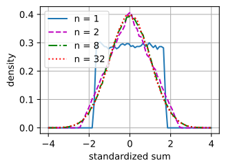
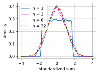
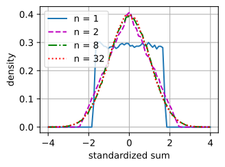
Watching universality happen. Like the Poisson limit, this claim is checkable in a few lines. The cell below starts from about the least Gaussian summand available (a \(U(0,1)\) draw, flat with hard edges and no tails), forms sums of \(n\) of them, standardizes each sum by its mean \(n/2\) and standard deviation \(\sqrt{n/12}\), and overlays the resulting histograms on the standard normal density. At \(n=1\) we see the uniform’s own plateau; at \(n=2\) the triangular hat; by \(n=8\) the curve is already hard to distinguish from the Gaussian, and at \(n=32\) the two agree to the resolution of the plot. Nothing in the code knows about the Gaussian: the bell is manufactured by the summation itself, which is exactly the universality the CLT asserts.
rng = np.random.default_rng(0)
ns, x = (1, 2, 8, 32), np.arange(-4, 4, 0.01)
curves = []
for n in ns:                                   # standardized sums of n uniforms
    s = (rng.random((100000, n)).sum(1) - n / 2) / np.sqrt(n / 12)
    hist, edges = np.histogram(s, bins=80, range=(-4, 4), density=True)
    curves.append(np.interp(x, (edges[:-1] + edges[1:]) / 2, hist))
curves.append(np.exp(-x**2 / 2) / np.sqrt(2 * np.pi))     # N(0, 1) density
d2l.plot(x, curves, xlabel='standardized sum', ylabel='density',
         legend=[f'n = {n}' for n in ns] + ['N(0, 1)'])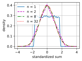
The normalizer and the moments. Why the constant \(1/\sqrt{2\pi\sigma^2}\)? The identity it rests on, \(\int_{-\infty}^\infty e^{-x^2/2}\,dx=\sqrt{2\pi}\), is the Gaussian integral computed in Section 25.4 by squaring the integral and passing to polar coordinates (Equation 25.4.10). Substituting \(x\mapsto(x-\mu)/\sigma\) then shows Equation 27.2.10 integrates to one. The parameters are the first two moments, and one integration by parts proves it: the mean is \(\mu\) by symmetry, and for the variance take \(\mu=0\), \(\sigma=1\) and integrate by parts with \(u=x\), \(dv=x\,e^{-x^2/2}\,dx\),
\[ \int_{-\infty}^{\infty} x^2\,\frac{e^{-x^2/2}}{\sqrt{2\pi}}\,dx = \frac{1}{\sqrt{2\pi}}\Bigl(\bigl[-x\,e^{-x^2/2}\bigr]_{-\infty}^{\infty} + \int_{-\infty}^{\infty} e^{-x^2/2}\,dx\Bigr) = 0 + 1 = 1, \]
so the standard Gaussian has variance \(1\); shifting by \(\mu\) and scaling by \(\sigma\) gives mean \(\mu\) and variance \(\sigma^2\) in general. (The exponential family’s moment property, Equation 27.2.16, will recover both by differentiation alone.)
Maximum entropy. Among all distributions with a given mean and variance, the Gaussian has the largest entropy: it is the most noncommittal choice consistent with knowing only those two numbers (Cover and Thomas 1999). We prove this in Section 28.1.2.3 as a short consequence of Gibbs’ inequality, and place it in context when we meet the exponential family below.
Where it arises. As the CLT limit it models aggregate noise; it is the noise model behind regression, where taking \(y\sim\mathcal N(\hat y,\sigma^2)\) makes the negative log-likelihood equal to mean squared error (Section 27.3.2.3); and it is the default prior and latent distribution throughout deep generative modeling.
import numpy as onp
rng = onp.random.default_rng(0)
mu, sigma = 0.0, 1.0
x = onp.arange(-4, 4, 0.01)
p = onp.exp(-(x - mu)**2 / (2 * sigma**2)) / onp.sqrt(2 * onp.pi * sigma**2)
print('total mass (≈1):', float((0.01 * p).sum().round(4)))
rng.normal(mu, sigma, size=(3, 3))              # sample from N(mu, sigma^2)
total mass (≈1): 0.9999array([[ 0.12573022, -0.13210486, 0.64042265],
[ 0.10490012, -0.53566937, 0.36159505],
[ 1.30400005, 0.94708096, -0.70373524]])27.2.2.4 Laplace
The Laplace distribution is a Gaussian’s sharper sibling: symmetric about a location \(\mu\), but with exponential decay on each side instead of Gaussian,
\[ p(x) = \frac{1}{2b}\,e^{-|x-\mu|/b}, \qquad X\sim\mathrm{Laplace}(\mu,b). \tag{27.2.11}\]
The two-sided exponential gives it a sharp peak at \(\mu\) and heavier tails than the Gaussian, visible in Figure 27.2.3.
Where it arises. The Laplace likelihood corresponds to the \(L_1\) loss, just as the Gaussian likelihood corresponds to squared error: its negative log-likelihood is proportional to \(|y-\hat y|\), the mean absolute error. As a prior on weights, it gives the sparsity-inducing regularizer \(\|\mathbf w\|_1\) used by LASSO (Tibshirani 1996).
Mean and variance. By symmetry \(\mu_X=\mu\). For the variance, center at \(\mu\) and use \(\int_0^\infty u^2 e^{-u}\,du=2\) with \(u=|x-\mu|/b\):
\[ \sigma_X^2 = \int_{-\infty}^\infty \frac{(x-\mu)^2}{2b}e^{-|x-\mu|/b}\,dx = \frac{2}{2b}\int_0^\infty x^2 e^{-x/b}\,dx = \frac{1}{b}\cdot b^3\!\int_0^\infty u^2 e^{-u}\,du = 2b^2 . \]
The location estimator makes the contrast concrete: the maximum-likelihood \(\hat\mu\) under a Laplace minimizes \(\sum_i|x_i-\mu|\), whose minimizer is the sample median (robust to outliers), whereas the Gaussian’s is the mean. The cell matches a Laplace and a Gaussian on variance and confirms the Laplace’s heavier tail by the fraction of mass beyond \(3\) standard deviations.
import numpy as onp
rng = onp.random.default_rng(0)
mu, b = 0.0, 1.0
sigma = onp.sqrt(2) * b                            # matched-variance Gaussian sd
U = (rng.random(200000) - 0.5) * (1 - 1e-7)       # open interval avoids log(0)
lap = mu - b * onp.sign(U) * onp.log(1 - 2 * onp.abs(U))  # inverse transform
gau = rng.normal(mu, sigma, 200000)
print('Laplace var (2b^2):', float(lap.var().round(3)), ' Gaussian var:', float(gau.var().round(3)))
print('P(|x| > 3sd): Laplace', float((onp.abs(lap) > 3 * sigma).mean()),
      ' Gaussian', float((onp.abs(gau) > 3 * sigma).mean()))
Laplace var (2b^2): 1.998 Gaussian var: 2.005
P(|x| > 3sd): Laplace 0.014575 Gaussian 0.0027227.2.2.5 Multivariate Gaussian
Almost every latent-variable and noise model in deep learning uses a Gaussian over a vector. The multivariate Gaussian \(\mathcal N(\boldsymbol\mu, \boldsymbol\Sigma)\) on \(\mathbb R^d\) has a mean vector \(\boldsymbol\mu\) and a symmetric positive-definite covariance matrix \(\boldsymbol\Sigma\), with density
\[ p(\mathbf x) = \frac{1}{(2\pi)^{d/2}|\boldsymbol\Sigma|^{1/2}} \exp\!\Bigl(-\tfrac12(\mathbf x-\boldsymbol\mu)^\top\boldsymbol\Sigma^{-1}(\mathbf x-\boldsymbol\mu)\Bigr). \tag{27.2.12}\]
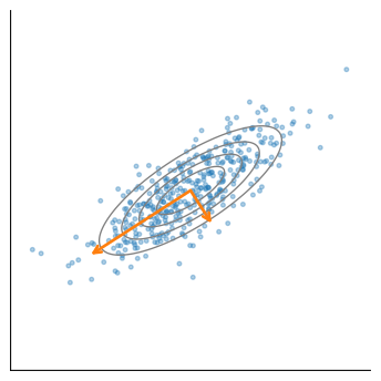
The geometry is the eigendecomposition. The exponent is a quadratic form in \(\boldsymbol\Sigma^{-1}\), so its level sets (the contours of equal density) are ellipsoids. The covariance \(\boldsymbol\Sigma\) is symmetric positive definite, so it has an orthonormal eigenbasis \(\boldsymbol\Sigma=\mathbf W\boldsymbol\Lambda\mathbf W^\top\) with all \(\lambda_i>0\) by the spectral theorem (Section 24.2.3.1), and the contour ellipsoid’s axes point along the eigenvectors \(\mathbf w_i\) with half-lengths proportional to \(\sqrt{\lambda_i}\): the principal directions of spread are the eigenvectors, stretched by the standard deviations along them. The isotropic case \(\boldsymbol\Sigma=\sigma^2\mathbf I\) gives spherical contours and factorizes into \(d\) independent one-dimensional Gaussians. Figure 27.2.4 draws this for a \(2\times2\) covariance.
It is the default vector noise and prior because it is closed under linear maps and conditioning. A linear transform \(\mathbf A\mathbf x+\mathbf b\) of a Gaussian is again Gaussian, with covariance \(\mathbf A\boldsymbol\Sigma\mathbf A^\top\); marginals (a special case, projecting onto a coordinate block) are therefore Gaussian too. Conditioning is closed in the same way. Partition the vector and its parameters into blocks \(\mathbf x=(\mathbf x_1,\mathbf x_2)\),
\[ \boldsymbol\mu = \begin{pmatrix}\boldsymbol\mu_1\\\boldsymbol\mu_2\end{pmatrix}, \qquad \boldsymbol\Sigma = \begin{pmatrix}\boldsymbol\Sigma_{11} & \boldsymbol\Sigma_{12}\\ \boldsymbol\Sigma_{21} & \boldsymbol\Sigma_{22}\end{pmatrix}, \]
and the conditional \(\mathbf x_1\mid\mathbf x_2\) is again Gaussian. We state its mean and covariance as a given fact (the derivation is a block-matrix computation, carried out in (Bishop 2006), §2.3; Exercise 10 puts the formulas to work):
\[ \boldsymbol\mu_{1\mid 2} = \boldsymbol\mu_1 + \boldsymbol\Sigma_{12}\boldsymbol\Sigma_{22}^{-1}(\mathbf x_2-\boldsymbol\mu_2), \qquad \boldsymbol\Sigma_{1\mid 2} = \boldsymbol\Sigma_{11} - \boldsymbol\Sigma_{12}\boldsymbol\Sigma_{22}^{-1}\boldsymbol\Sigma_{21}. \tag{27.2.13}\]
The conditional mean is a linear function of the observed block (a linear regression of \(\mathbf x_1\) on \(\mathbf x_2\) read straight off the covariance), and the conditional covariance \(\boldsymbol\Sigma_{11}-\boldsymbol\Sigma_{12}\boldsymbol\Sigma_{22}^{-1}\boldsymbol\Sigma_{21}\) is the Schur complement of \(\boldsymbol\Sigma_{22}\), the block that remains when the variables in \(\mathbf x_2\) are eliminated. It does not depend on the observed value \(\mathbf x_2\). These formulas underlie Gaussian process regression (Chapter 21): conditioning the joint Gaussian prior over function values on the observations gives the predictive mean and variance.
Sampling via Cholesky. How do we draw from \(\mathcal N(\boldsymbol\mu,\boldsymbol\Sigma)\) given only a standard-normal generator? This is the application promised when the Cholesky factorization was introduced (Section 24.2.3.2): factor \(\boldsymbol\Sigma=\mathbf L\mathbf L^\top\) with \(\mathbf L\) lower triangular, draw \(\mathbf z\sim\mathcal N(\mathbf 0,\mathbf I_d)\) (\(d\) independent standard normals), and set \(\mathbf x=\boldsymbol\mu+\mathbf L\mathbf z\). Then \(\mathbf x\) is Gaussian (a linear map of a Gaussian), and its mean is \(\boldsymbol\mu\) because \(\mathbb E[\mathbf z]=\mathbf 0\). Its covariance is
\[ \mathbb E\bigl[(\mathbf x-\boldsymbol\mu)(\mathbf x-\boldsymbol\mu)^\top\bigr] = \mathbf L\,\mathbb E[\mathbf z\mathbf z^\top]\,\mathbf L^\top = \mathbf L\,\mathbf I\,\mathbf L^\top = \boldsymbol\Sigma . \]
This recipe is what the library samplers run: \(d\) standard normals plus one triangular matrix multiply. The cell draws samples through the library sampler, estimates the covariance, checks that its eigenvalues recover the \(\{1,3\}\) built into \(\boldsymbol\Sigma\), then re-samples by the Cholesky recipe and confirms that it reproduces \(\boldsymbol\Sigma\) as well.
import numpy as onp
rng = onp.random.default_rng(0)
mu_v = onp.array([0., 0.])
Sigma = onp.array([[2., 1.], [1., 2.]])
sample = rng.multivariate_normal(mu_v, Sigma, size=5000)
emp = onp.cov(sample.T)
vals, vecs = onp.linalg.eigh(emp)
print('empirical covariance:\n', emp.round(2))
print('eigenvalues (≈ 1, 3):', vals.round(2))   # Sigma has eigenvalues 1 and 3
L = onp.linalg.cholesky(Sigma)                   # Sigma = L L^T
chol = mu_v + rng.standard_normal((5000, 2)) @ L.T  # x = mu + L z
print('Cholesky-recipe covariance:\n', onp.cov(chol.T).round(2))
empirical covariance:
[[1.96 1.03]
[1.03 2.06]]
eigenvalues (≈ 1, 3): [0.98 3.04]
Cholesky-recipe covariance:
[[1.93 0.97]
[0.97 2. ]]Probability in high dimension. One more Gaussian fact matters enormously in deep learning and defies low-dimensional intuition. For \(\mathbf x\sim\mathcal N(\mathbf 0,\mathbf I_d)\) the squared norm \(\|\mathbf x\|^2=\sum_{i=1}^d x_i^2\) is a sum of \(d\) independent terms with mean \(1\), so \(\mathbb E\,\|\mathbf x\|^2=d\), and, by the same averaging that makes sample means reliable, the sum concentrates near \(d\): virtually all the mass of a high-dimensional Gaussian lives in a thin shell of radius \(\approx\sqrt d\), far from the origin where the density is pointwise largest. Likewise two independent draws \(\mathbf x,\mathbf y\) are nearly orthogonal: their cosine has mean \(0\) and standard deviation \(\approx1/\sqrt d\), a probabilistic version of the concentration-of-angles proposition of Section 24.1; both facts get their full quantitative treatment, with exponential tail bounds, in Section 27.6. Both matter in practice: weight-initialization schemes scale by \(1/\sqrt{d}\) precisely so that \(\|\mathbf W\mathbf x\|\) stays comparable to \(\|\mathbf x\|\) layer after layer; cosine similarity between embeddings is informative because unrelated high-dimensional vectors sit near cosine \(0\) by default; and nearest-neighbor search loses contrast because the distances between random points all concentrate around one common value. The check below watches both concentrations set in as \(d\) grows.
rng = np.random.default_rng(0)
for d in (3, 30, 300):
    x, y = rng.standard_normal((2, 1000, d))
    nx = np.linalg.norm(x, axis=1)
    cos = (x * y).sum(1) / (nx * np.linalg.norm(y, axis=1))
    print(f'd = {d:3d}:  ||x||/sqrt(d) = {(nx / np.sqrt(d)).mean():.3f}'
          f' ± {(nx / np.sqrt(d)).std():.3f},   mean |cos(x,y)| = {np.abs(cos).mean():.3f}')
d = 3: ||x||/sqrt(d) = 0.920 ± 0.378, mean |cos(x,y)| = 0.497
d = 30: ||x||/sqrt(d) = 0.992 ± 0.127, mean |cos(x,y)| = 0.145
d = 300: ||x||/sqrt(d) = 1.000 ± 0.039, mean |cos(x,y)| = 0.046The norm ratio locks onto \(1\) with a spread shrinking like \(1/\sqrt{2d}\), and the typical cosine collapses toward \(0\) at the promised \(1/\sqrt d\) rate: in high dimension, Gaussian geometry is a thin shell of mutually near-orthogonal directions.
27.2.3 The Exponential Family
Nearly every distribution above (Bernoulli, categorical, binomial, Poisson, exponential, Gaussian, Laplace with fixed location) is a special case of one form, the exponential family. A distribution belongs to it if its density (or mass) can be written
\[ p(\mathbf x\mid\boldsymbol\eta) = h(\mathbf x)\,\exp\!\bigl(\boldsymbol\eta^\top T(\mathbf x) - A(\boldsymbol\eta)\bigr). \tag{27.2.14}\]
The four ingredients each play a clear role. The base measure \(h(\mathbf x)\) is a fixed background that does not depend on the parameters. The natural parameters \(\boldsymbol\eta\) are the knobs. The sufficient statistics \(T(\mathbf x)\) are the only features of the data that matter: given \(T(\mathbf x)\), no other detail of \(\mathbf x\) affects the probability, which is exactly what “sufficient” means. The log-partition function (or cumulant function)
\[ A(\boldsymbol\eta) = \log\!\int h(\mathbf x)\,\exp\!\bigl(\boldsymbol\eta^\top T(\mathbf x)\bigr)\,d\mathbf x \tag{27.2.15}\]
is whatever it takes to make Equation 27.2.14 integrate to one.
27.2.3.1 Identifying Standard Distributions
The form looks abstract until we match the pieces. The Bernoulli \(p^x(1-p)^{1-x}\) rewrites as
\[ \exp\!\Bigl(x\log\tfrac{p}{1-p} + \log(1-p)\Bigr), \]
so \(T(x)=x\), the natural parameter \(\eta=\log\tfrac{p}{1-p}\) is the logit, and \(A(\eta)=\log(1+e^\eta)\) is the softplus; the link between probabilities and logits is built into the family. The Poisson \(\tfrac{\lambda^k e^{-\lambda}}{k!}\) has base measure \(h(k)=1/k!\), statistic \(T(k)=k\), parameter \(\eta=\log\lambda\), and \(A(\eta)=e^\eta=\lambda\). The Gaussian with unknown mean and variance is a two-parameter member: completing the exponent,
\[ \frac{1}{\sqrt{2\pi}}\exp\!\Bigl(\underbrace{\tfrac{\mu}{\sigma^2}}_{\eta_1}\,x + \underbrace{\bigl(-\tfrac{1}{2\sigma^2}\bigr)}_{\eta_2}\,x^2 - \underbrace{\bigl(\tfrac{\mu^2}{2\sigma^2}+\log\sigma\bigr)}_{A(\boldsymbol\eta)}\Bigr), \]
so \(T(x)=(x,x^2)^\top\) with base measure \(h(x)=1/\sqrt{2\pi}\). The second natural parameter is negative, \(\eta_2=-1/(2\sigma^2)<0\), which is what forces the tail-suppressing \(e^{-x^2}\) decay. The exact split between \(h\), \(\eta\), and \(T\) is not unique; what matters is that the distribution fits the form at all.
Membership has edges. The conspicuous absentees from the list above are the two uniforms: when the endpoints are unknown parameters, the support of \(U(a,b)\) (and likewise of \(U(n)\)) moves with those parameters, whereas every member of Equation 27.2.14 has the fixed, parameter-free support of its base measure \(h\). This is the classic counterexample. Heavy-tailed laws live outside the family for a different reason. The Student-\(t\) takes two lines to define: draw a random precision \(1/\sigma^2\) from a Gamma distribution (a two-parameter density on the positive half-line, defined in full among the conjugate priors below), then draw a Gaussian with that precision. Averaging the Gaussian over its random scale fattens the \(e^{-x^2}\) tails into polynomial ones, and the Cauchy of Section 27.1 is its one-degree-of-freedom extreme. The support here is all of \(\mathbb R\), fixed, yet the mixing destroys the exponential form: no fixed finite-dimensional sufficient statistic exists, the situation described by the Pitman–Koopman–Darmois theorem (Bishop 2006). The exclusion costs two conveniences: these laws admit no finite-dimensional conjugate prior, and their negative log-likelihoods are not convex in the parameters. Both conveniences are exponential-family privileges, as the rest of this section shows.
27.2.3.2 Maximum-Entropy Derivation
Maximum entropy produces an exponential-family form only relative to a chosen support, base measure, and feasible set of constraints. Fix a base measure \(h\), require \(p\) to be absolutely continuous with respect to it, and impose normalization together with \(\mathbb E_p[T(\mathbf x)]=\boldsymbol\tau\). If the constraints are feasible, the log-partition function is finite, and a maximizer exists in the regular interior case, the optimizer has the exponential form below. Existence can fail for incompatible constraints or heavy-tailed settings.
The two maximum-entropy facts cited earlier (Cover and Thomas 1999) are the same statement seen twice: the discrete uniform is the maximum-entropy distribution on a finite set when we fix nothing but the support, and the Gaussian is the maximum-entropy distribution on the line when we fix the mean and variance. In general, maximizing the entropy relative to the base measure \(h\), \(H_h[p]=-\int p\log\tfrac{p}{h}\), subject to fixing the expected sufficient statistics \(\mathbb E[T(\mathbf x)]=\boldsymbol\tau\) has, by a Lagrange multiplier argument (Section 26.4.1), the solution
\[ p(\mathbf x) \propto h(\mathbf x)\,\exp\!\bigl(\boldsymbol\eta^\top T(\mathbf x)\bigr), \]
which is precisely Equation 27.2.14: the multipliers \(\boldsymbol\eta\) are the natural parameters and \(A(\boldsymbol\eta)\) is again the normalizer (Murphy 2022; Wainwright and Jordan 2008). One subtlety: the base measure does real work here. With plain Shannon entropy, i.e. \(h\equiv1\), fixing the mean on \(\{0,1,2,\dots\}\) yields the geometric distribution; only entropy relative to \(h(k)=1/k!\) yields the Poisson. For the uniform and the Gaussian above, \(h\) is constant, so plain entropy was the relevant objective in those cases. Thus, when the optimization problem has a solution, the solution is least committal only relative to the selected support, base measure, entropy, and moment constraints. Changing those choices can change the optimizer.
27.2.3.3 The Moment Property
The single most useful fact about Equation 27.2.14 is that \(A\) is a moment generator: differentiating the log-partition function returns the mean of the sufficient statistics.
Proposition (mean of the sufficient statistics). For an exponential-family distribution Equation 27.2.14,
\[ \nabla_{\boldsymbol\eta} A(\boldsymbol\eta) = \mathbb E[T(\mathbf x)]. \tag{27.2.16}\]
Proof. Differentiate Equation 27.2.15 under the integral sign; we grant the interchange of derivative and integral, which is valid on the interior of the natural-parameter domain (Folland 1999). Writing \(Z(\boldsymbol\eta)=e^{A(\boldsymbol\eta)}=\int h(\mathbf x)e^{\boldsymbol\eta^\top T(\mathbf x)}d\mathbf x\), the derivative of the log is \(\nabla A = (\nabla Z)/Z\), and
\[ \nabla_{\boldsymbol\eta} Z = \int h(\mathbf x)\,T(\mathbf x)\,e^{\boldsymbol\eta^\top T(\mathbf x)}\,d\mathbf x . \]
Dividing by \(Z=e^{A}\) pulls the \(e^{-A}\) back inside, reconstituting the density Equation 27.2.14:
\[ \nabla_{\boldsymbol\eta} A = \frac{1}{Z}\int h(\mathbf x)\,T(\mathbf x)\,e^{\boldsymbol\eta^\top T(\mathbf x)}\,d\mathbf x = \int T(\mathbf x)\,\underbrace{h(\mathbf x)\,e^{\boldsymbol\eta^\top T(\mathbf x) - A(\boldsymbol\eta)}}_{p(\mathbf x\mid\boldsymbol\eta)}\,d\mathbf x = \mathbb E[T(\mathbf x)] . \quad\blacksquare \]
Differentiating once more (the same interchange) turns \(\nabla A=(\nabla Z)/Z\) into
\[ \nabla^2 A = \frac{\nabla^2 Z}{Z} - \frac{(\nabla Z)(\nabla Z)^\top}{Z^2} = \mathbb E[T\,T^\top] - \mathbb E[T]\,\mathbb E[T]^\top = \operatorname{Cov}(T), \]
so \(A\) is convex (a covariance matrix is PSD, Section 24.2.3.2). Consequently, for a sample \(x_1,\dots,x_n\) the negative log-likelihood is
\[ -\sum_{i=1}^{n} \log p(x_i\mid\boldsymbol\eta) = n\,A(\boldsymbol\eta) - \boldsymbol\eta^\top \sum_{i=1}^{n} T(x_i) - \sum_{i=1}^{n} \log h(x_i), \]
convex in \(\boldsymbol\eta\) because \(A\) is. Setting its gradient to zero gives \(n\nabla A(\boldsymbol\eta)=\sum_i T(x_i)\): by the moment property, maximum likelihood matches the model’s expected sufficient statistics to their empirical averages, \(\mathbb E[T]=\bar T\). Uniqueness of the optimum needs one more hypothesis, strict convexity: \(\operatorname{Cov}(T)\succ0\), which holds when the representation is minimal (no linear combination of the sufficient statistics is constant). The section’s own softmax parameterization Equation 27.2.3 is not minimal: adding the same constant to every logit leaves every \(p_k\) unchanged, so the categorical negative log-likelihood is flat along the direction \(\mathbf 1\) and its optima form a line rather than a point, which is why implementations pin the shift (fixing one logit at zero, or subtracting the maximum). We verify Equation 27.2.16 for the Bernoulli, where it should read \(A'(\eta)=\sigma(\eta)=\mathbb E[x]=p\).
import numpy as onp
eta = 0.7                                        # natural parameter (logit)
A = lambda e: onp.log1p(onp.exp(e))                # Bernoulli log-partition (softplus)
eps = 1e-6
dA = (A(eta + eps) - A(eta - eps)) / (2 * eps)   # numerical dA/deta
print('dA/deta      =', round(float(dA), 6))
print('sigmoid(eta) = E[x] = p =', round(float(1 / (1 + onp.exp(-eta))), 6))
dA/deta = 0.668188
sigmoid(eta) = E[x] = p = 0.668188The derivative of the softplus is the sigmoid, and it lands exactly on the Bernoulli mean \(p\). This is no coincidence: the sigmoid and softmax links that deep-learning classifiers use are precisely the maps from natural parameters to means in the Bernoulli and categorical families, and the convexity of \(A\) is why their negative log-likelihoods are convex in the natural parameters. If those parameters are affine functions of fixed features, this gives a convex optimization problem. A neural network makes the natural parameters nonlinear functions of its weights, so the same loss is not generally convex in the weights. The exponential family still supplies the likelihood and the link functions used by standard deep-learning losses (Bishop 2006; Koller and Friedman 2009).
27.2.4 Conjugate Priors
The distributions above model observations, but Bayesian inference also requires distributions over their parameters: the Bernoulli probability \(p\), the Poisson rate \(\lambda\), or the categorical probability vector \(\mathbf p\). Such a distribution is a prior. Three continuous distributions provide the standard priors for the discrete likelihoods introduced above: the Beta, Gamma, and Dirichlet distributions.
A prior is conjugate to a likelihood if the posterior belongs to the same family as the prior. Observations then update the parameters of the distribution without changing its functional form. The dashed links in Figure 27.2.1 show these conjugate pairs.
27.2.4.1 Beta–Bernoulli Conjugacy and Pseudo-Counts
The Beta distribution is a density on the unit interval \(p\in[0,1]\) (exactly the range of a probability) with two shape parameters \(\alpha,\beta>0\),
\[ \mathrm{Beta}(p\mid\alpha,\beta) = \frac{p^{\alpha-1}(1-p)^{\beta-1}}{B(\alpha,\beta)}, \tag{27.2.17}\]
where the normalizing constant is \(B(\alpha,\beta)=\Gamma(\alpha)\Gamma(\beta)/\Gamma(\alpha+\beta)\), with \(\Gamma\) the Gamma function that the exercises of Section 25.4 introduced (recall \(\Gamma(z+1)=z\,\Gamma(z)\) and \(\Gamma(n+1)=n!\)). The mean follows from this normalizer:
\[ \mathbb E[p] = \frac{1}{B(\alpha,\beta)}\int_0^1 p^{\alpha}(1-p)^{\beta-1}\,dp = \frac{B(\alpha+1,\beta)}{B(\alpha,\beta)} = \frac{\alpha}{\alpha+\beta}, \]
using \(\Gamma(\alpha+1)=\alpha\,\Gamma(\alpha)\) to simplify the ratio; the same move one step further gives the variance \(\operatorname{Var}(p)=\alpha\beta/\bigl((\alpha+\beta)^2(\alpha+\beta+1)\bigr)\). The uniform prior on \([0,1]\) that Section 27.3 will place on the coin’s bias is the special case \(\alpha=\beta=1\).
Now take a Beta prior on a coin’s bias \(p\) and observe a Bernoulli/binomial sample with \(x\) heads in \(n\) flips. Multiplying the prior by the likelihood Equation 27.2.6,
\[ \underbrace{p^{\alpha-1}(1-p)^{\beta-1}}_{\text{prior}}\cdot \underbrace{p^{x}(1-p)^{n-x}}_{\text{likelihood}} = p^{(\alpha+x)-1}(1-p)^{(\beta+n-x)-1}, \]
which, up to normalization, is again a Beta, now with parameters shifted by the data:
\[ p \mid x \;\sim\; \mathrm{Beta}\bigl(\alpha+x,\ \beta+(n-x)\bigr). \tag{27.2.18}\]
This update has a pseudo-count interpretation. The parameters \(\alpha\) and \(\beta\) act as prior counts for heads and tails. Observing \(x\) heads and \(n-x\) tails adds these observations to the corresponding prior counts. The posterior mean
\[ \mathbb E[p\mid x] = \frac{\alpha+x}{\alpha+\beta+n} \]
is the empirical frequency after including the pseudo-counts. It lies between the prior mean \(\alpha/(\alpha+\beta)\) and the maximum-likelihood estimate \(x/n\), and approaches the latter as \(n\) grows. With the uniform prior \(\alpha=\beta=1\) it becomes Laplace’s rule of succession \((x+1)/(n+2)\) (Laplace 1814): estimate a probability by adding one phantom observation of each outcome. The cell verifies the update on a small sample.
alpha, beta = 2.0, 2.0                           # Beta prior pseudo-counts
x, n = 7, 10                                     # 7 heads in 10 flips
post_alpha, post_beta = alpha + x, beta + (n - x)  # Beta posterior update
print('prior mean      =', round(alpha / (alpha + beta), 4))
print('MLE  x/n        =', round(x / n, 4))
print('posterior Beta  =', (post_alpha, post_beta))
print('posterior mean  =', round(post_alpha / (post_alpha + post_beta), 4))
prior mean = 0.5
MLE x/n = 0.7
posterior Beta = (9.0, 5.0)
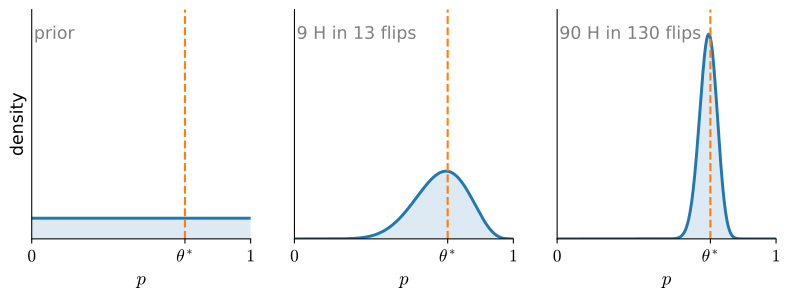
posterior mean = 0.6429The posterior mean lies between the prior mean \(0.5\) and the empirical frequency \(0.7\), as the pseudo-count calculation predicts. Figure 27.2.5 shows the same update with more data: the flat \(\mathrm{Beta}(1,1)\) prior becomes concentrated around the true bias, and its width decreases as \(1/\sqrt n\).
27.2.4.2 Other Conjugate Pairs
The other discrete laws have their own conjugate partners, built the same way.
Gamma–Poisson. The Gamma distribution \(\mathrm{Gamma}(\lambda\mid\alpha,\beta)=\frac{\beta^\alpha}{\Gamma(\alpha)}\,\lambda^{\alpha-1}e^{-\beta\lambda}\) is a density on the rate \(\lambda>0\) with mean \(\alpha/\beta\) and variance \(\alpha/\beta^2\). Its conjugacy with the Poisson follows by the same multiplication used for the Beta: \(n\) observed counts \(x_1,\dots,x_n\) contribute the likelihood \(\propto\lambda^{\sum_i x_i}e^{-n\lambda}\), and multiplying by the prior collects powers into \(\lambda^{\alpha+\sum_i x_i-1}e^{-(\beta+n)\lambda}\), the posterior \(\mathrm{Gamma}\bigl(\alpha+\sum_i x_i,\ \beta+n\bigr)\): pseudo-events over a pseudo-window. Averaging the Poisson over this Gamma uncertainty in its rate yields the negative binomial, the over-dispersed fix promised in the Poisson section.
Gamma as a waiting time. The Gamma is more than a prior: with integer shape \(\alpha=k\), \(\mathrm{Gamma}(k,\beta)\) is the waiting time to the \(k\)-th event of the Poisson process we named at the bus stop, the sum of \(k\) independent \(\mathrm{Exp}(\beta)\) waits, extending the exponential’s arrow in the family tree just as the binomial extends the Bernoulli’s.
Dirichlet–Multinomial. The Dirichlet distribution
\[ \mathrm{Dir}(\mathbf p\mid\boldsymbol\alpha)=\frac{\Gamma(\sum_k\alpha_k)}{\prod_k\Gamma(\alpha_k)}\prod_k p_k^{\alpha_k-1} \]
is the multivariate Beta, a density over probability vectors on the simplex, with mean \(\mathbb E[p_k]=\alpha_k/\sum_j\alpha_j\). It is conjugate to the categorical/multinomial by the same multiplication: the likelihood contributes \(\prod_k p_k^{x_k}\), so observing class counts \(\mathbf x\) updates the prior to \(\mathrm{Dir}(\boldsymbol\alpha+\mathbf x)\), one pseudo-count per class.
These are three instances of one theorem. Every exponential-family likelihood has a conjugate prior, provided the hyperparameters are chosen so that the prior below is normalizable, and that prior is itself an exponential family in the natural parameters \(\boldsymbol\eta\): writing the prior as \(p(\boldsymbol\eta)\propto\exp\!\bigl(\boldsymbol\nu^\top\boldsymbol\eta - \kappa\,A(\boldsymbol\eta)\bigr)\), Multiplying by the likelihood Equation 27.2.14 adds the data’s sufficient statistics to \(\boldsymbol\nu\) and increments \(\kappa\) by the sample size. The pseudo-count update of Equation 27.2.18 is this general mechanism specialized to the Bernoulli, and the hyperparameters \((\boldsymbol\nu,\kappa)\) are pseudo-data: a prior sufficient statistic and a prior sample size (Bishop 2006; Murphy 2022). Conjugacy makes the exponential family the natural home of tractable Bayesian inference as well as of the standard losses.
27.2.5 Summary
Here are the eleven data distributions of this section in one view; their three conjugate priors, the Beta, Gamma, and Dirichlet, close the family. For the categorical and multinomial rows we code a draw as a one-hot vector, respectively as the sum of \(n\) one-hot vectors: the coding the cross-entropy loss already uses, and the object whose mean and covariance the table states.
| Law | pmf or pdf | Mean | Variance | Where it shows up in DL |
|---|---|---|---|---|
| \(\mathrm{Bernoulli}(p)\) | \(p^x(1-p)^{1-x}\) | \(p\) | \(p(1-p)\) | binary classifier output, BCE loss |
| \(\mathrm{Categorical}(\mathbf p)\) | \(p_k\) | \(\mathbf p\) | \(\operatorname{diag}(\mathbf p)-\mathbf p\mathbf p^\top\) | softmax output, cross-entropy loss |
| \(\mathrm{Multinomial}(n,\mathbf p)\) | Equation 27.2.4 | \(n\mathbf p\) | \(n\bigl(\operatorname{diag}(\mathbf p)-\mathbf p\mathbf p^\top\bigr)\) | class counts over \(n\) draws |
| Uniform \(U(n)\) | \(1/n\) | \((n+1)/2\) | \((n^2-1)/12\) | index sampling, shuffling |
| \(\mathrm{Binomial}(n,p)\) | \(\binom nk p^k(1-p)^{n-k}\) | \(np\) | \(np(1-p)\) | success counts over \(n\) trials |
| \(\mathrm{Poisson}(\lambda)\) | \(\lambda^k e^{-\lambda}/k!\) | \(\lambda\) | \(\lambda\) | rare-event counts |
| Uniform \(U(a,b)\) | \(1/(b-a)\) on \([a,b]\) | \((a+b)/2\) | \((b-a)^2/12\) | raw randomness, initialization |
| \(\mathrm{Exp}(\lambda)\) | \(\lambda e^{-\lambda x}\), \(x\ge0\) | \(1/\lambda\) | \(1/\lambda^2\) | waiting times, survival |
| \(\mathcal N(\mu,\sigma^2)\) | \(\frac{1}{\sqrt{2\pi\sigma^2}}e^{-(x-\mu)^2/2\sigma^2}\) | \(\mu\) | \(\sigma^2\) | MSE noise model, CLT, priors |
| \(\mathrm{Laplace}(\mu,b)\) | \(\frac{1}{2b}e^{-\lvert x-\mu\rvert/b}\) | \(\mu\) | \(2b^2\) | MAE loss, \(L_1\) sparsity prior |
| \(\mathcal N(\boldsymbol\mu,\boldsymbol\Sigma)\) | Equation 27.2.12 | \(\boldsymbol\mu\) | \(\boldsymbol\Sigma\) | latent priors, Gaussian processes |
- Distributions form a family: Bernoulli is the seed; summing \(n\) gives the Binomial (\(\mu=np\), \(\sigma^2=np(1-p)\), derived as a sum of Bernoullis); the many-rare limit gives the Poisson (\(\mu=\sigma^2=\lambda\), derived from the binomial); the many-ordinary limit (CLT) gives the Gaussian.
- The Categorical generalizes Bernoulli to \(K\) outcomes; its softmax form is every classifier’s output layer and its NLL is the cross-entropy loss. The Multinomial counts \(n\) categorical draws.
- The continuous laws: the uniform (raw randomness, \(U(0,1)\) powers sampling), the exponential (memoryless waiting times, partner of the Poisson), the Gaussian (CLT limit, MSE noise model, max-entropy default), the Laplace (\(L_1\)/MAE loss, sparsity prior), and the multivariate Gaussian, whose elliptical contours are the eigendecomposition of its covariance, which is closed under both linear maps and conditioning (the Schur-complement formulas, Equation 27.2.13, that drive Gaussian-process regression), and which is sampled by the Cholesky recipe \(\mathbf x=\boldsymbol\mu+\mathbf L\mathbf z\).
- Means and variances follow from structure (linearity of expectation, limits, and standard integrals) rather than memorization.
- The exponential family \(p(\mathbf x)=h(\mathbf x)\exp(\boldsymbol\eta^\top T(\mathbf x)-A(\boldsymbol\eta))\) unifies almost all of them (the uniforms, whose support moves with their parameters, stay outside). Under feasible moment constraints and regularity conditions, the form arises by maximizing entropy relative to a selected base measure \(h\). Its log-partition \(A\) generates moments: \(\nabla A(\boldsymbol\eta)=\mathbb E[T(\mathbf x)]\), and \(A\) is convex. Thus its negative log-likelihood is convex in the natural parameters; with an affine parameter map this yields a convex generalized linear model, whereas a neural-network parameterization remains nonconvex.
- Every exponential-family likelihood has a conjugate prior: the Beta for the Bernoulli/binomial, the Gamma for the Poisson, the Dirichlet for the categorical/multinomial. Bayesian updating then just adds the data’s sufficient statistics to the prior’s pseudo-counts: e.g. a \(\mathrm{Beta}(\alpha,\beta)\) prior and \(x\) heads in \(n\) flips give a \(\mathrm{Beta}(\alpha+x,\beta+n-x)\) posterior.
27.2.6 Exercises
- Let \(X,Y\sim\mathrm{Binomial}(16,1/2)\) be independent. Find the standard deviation of \(X-Y\). (Hint: variances add for independent variables, even under subtraction.)
- Show that the categorical negative log-likelihood \(-\sum_k y_k\log p_k\) with \(p_k\) from the softmax Equation 27.2.3 has gradient \(\hat{\mathbf p}-\mathbf y\) with respect to the logits \(\mathbf z\). Why does this form make softmax classification well behaved?
- Verify that the multinomial pmf Equation 27.2.4 for \(n\) trials, \(K=2\), reduces exactly to the binomial pmf Equation 27.2.6.
- Prove the converse of memorylessness: if a positive continuous random variable has survival function \(G(t)=P(X>t)\) satisfying \(G(s+t)=G(s)\,G(t)\) for all \(s,t\ge0\), show that \(G(t)=e^{-\lambda t}\) for some \(\lambda>0\) (use monotonicity of \(G\)). Then show that the minimum of independent \(\mathrm{Exp}(\lambda_i)\) is again exponential with rate \(\sum_i\lambda_i\).
- For \(X\sim\mathrm{Poisson}(\lambda)\), argue that \((X-\lambda)/\sqrt\lambda\) becomes approximately Gaussian as \(\lambda\to\infty\). (Hint: for integer \(\lambda=m\), a \(\mathrm{Poisson}(m)\) variable is the sum of \(m\) independent \(\mathrm{Poisson}(1)\) variables, so the iid CLT applies as \(m\to\infty\); general \(\lambda\) follows by splitting off the fractional part.)
- Show that the maximum-likelihood location \(\mu\) under a \(\mathrm{Laplace}(\mu,b)\) model minimizes \(\sum_i|x_i-\mu|\) and hence is the sample median, while under a Gaussian it is the mean.
- Write the categorical distribution over \(K\) classes in exponential-family form Equation 27.2.14. Identify \(T(\mathbf x)\) (one-hot) and the natural parameters, and verify that \(\nabla A(\boldsymbol\eta)=\mathbb E[T]\) recovers the softmax Equation 27.2.3.
- Given \(\boldsymbol\Sigma=\left(\begin{smallmatrix}2&1\\1&2\end{smallmatrix}\right)\), find the eigenvalues and eigenvectors and state the axis directions and half-lengths of the \(\mathcal N(\mathbf 0,\boldsymbol\Sigma)\) density contours. Show that a linear map \(\mathbf A\mathbf x+\mathbf b\) of a multivariate Gaussian is again Gaussian with covariance \(\mathbf A\boldsymbol\Sigma\mathbf A^\top\).
- Start from a uniform \(\mathrm{Beta}(1,1)\) prior on a coin’s bias and observe the sequence “HHHTHTTHHHHHT” (\(9\) heads, \(4\) tails) of Section 27.3. Give the posterior Equation 27.2.18 and its mean, and show that as the data grows the posterior mean converges to the maximum-likelihood frequency \(n_H/(n_H+n_T)\).
- Using the conditional formula Equation 27.2.13, take the bivariate Gaussian with \(\boldsymbol\mu=\mathbf 0\) and \(\boldsymbol\Sigma=\left(\begin{smallmatrix}1&\rho\\\rho&1\end{smallmatrix}\right)\) and find the distribution of \(x_1\) given \(x_2\). Show its mean is \(\rho x_2\) and its variance is \(1-\rho^2\), and explain why observing \(x_2\) never increases the uncertainty about \(x_1\).