%matplotlib inline
from d2l import torch as d2l
import json
import os
import pathlib
import subprocess
import sys
import time
import torch
from torch import nn
import torch.nn.functional as F
import torch.utils.checkpoint as ckpt

torch.set_float32_matmul_precision('high')
# The profiler's CUDA instrumentation must not outlive its cell — without
# this, every timing after the first profile pays a per-launch tax.
os.environ['TEARDOWN_CUPTI'] = '1'13.7 Case Study: Optimizing a Transformer
This section applies the chapter’s method to the GPT model of Section 11.2. We profile a baseline, classify its limiting regime, apply one optimization, and profile again before choosing the next step. The sequence includes compilation, reduced precision, larger batches, activation checkpointing, and data parallelism. Reporting each incremental change separates the contribution of a technique from interactions among techniques.
Prerequisites: the entire chapter. The subject is d2l.GPT and d2l.TimeMachine from Section 11.2, reused verbatim.
%matplotlib inline
from d2l import jax as d2l
from flax import nnx
import jax
from jax import numpy as jnp
import optax
import os
import time

# XLA's NCCL buffer registration fails harmlessly on this P2P-less box;
# opt out rather than let every collective print the warning (see 13.6).
os.environ.setdefault('NCCL_LOCAL_REGISTER', '0')'0'13.7.1 The Subject
We take ch. 11’s GPT at a width where the experiment can be read cleanly.
At the num_hiddens=256 of Section 11.2, the model’s matmuls are small enough that some techniques do not clear the measurement noise — worse, bf16 actively hurts, because width-256 matmuls are too small to feed the tensor cores and the casting overhead dominates (an instructive failure, pursued in the exercises). Widening to num_hiddens=512 (about 19M parameters, six blocks, char-level Time Machine, context 128) puts each measured effect above the timing noise floor. The metric is training throughput in tokens per second, measured with the discipline of Section 13.1.
At the num_hiddens=256 of Section 11.2 the matmuls are small enough that several configurations would sit inside the measurement noise; widening to num_hiddens=512 (about 19M parameters, six blocks, char-level Time Machine, context 128) gives every real effect room to show. The metric is training throughput in tokens per second, measured with the discipline of Section 13.1.
The case study runs in both frameworks, deliberately in parallel: the same model, data, metric, and measurement protocol. The optimization sequences diverge where the frameworks do — what compiled execution means, which change the profile suggests next, and how data parallelism is launched — and that divergence is itself part of the closing lesson: the method transfers; the recipe does not.
The benchmark contract is fixed throughout the section:
| field | setting |
|---|---|
| hardware | this book’s four 24-GB RTX 4090 GPUs; single-GPU tests use one card |
| model | six GPT blocks, width 512, character vocabulary, context 128 |
| data | Time Machine batches, reshuffled; incomplete batches are dropped |
| optimizer | AdamW at \(10^{-3}\) unless a cell states otherwise |
| metric | end-to-end training tokens/s, including input staging and optimizer update |
| timing | fixed shapes, synchronization, 60 warm-up and 100 timed steps by default |
| precision | fp32 baseline with documented tf32 policy; bf16 changes are explicit |
Each displayed throughput is one timed window, so the reported ratios describe this host and shape rather than a hardware-independent ranking.
device = d2l.try_gpu()
data = d2l.TimeMachine(batch_size=64, num_steps=128, tokenization='char')
vocab_size = len(data.vocab)

def make_gpt():
    torch.manual_seed(0)
    return d2l.GPT(vocab_size, num_hiddens=512, num_blks=6).to(device)

model = make_gpt()
print(f'{sum(p.numel() for p in model.parameters()) / 1e6:.1f}M parameters')

def batches(dm):
    while True:
        for X, Y in dm.train_dataloader():
            if X.shape[0] == dm.batch_size:   # constant shape: no retrace
                yield X.to(device), Y.to(device)
stream = batches(data)
18.9M parametersdata = d2l.TimeMachine(batch_size=64, num_steps=128, tokenization='char')
vocab_size = len(data.vocab)
def make_gpt():
return d2l.GPT(vocab_size, num_hiddens=512, num_blks=6,
rngs=nnx.Rngs(0))
model = make_gpt()
n_params = sum(p.size for p in jax.tree.leaves(nnx.state(model, nnx.Param)))
print(f'{n_params / 1e6:.1f}M parameters')
def batches(dm, batch_size=None, seed=0):
"""Shuffled minibatches, staged on device once (the corpus is 5 MB)."""
X, Y = jnp.asarray(dm.X[:dm.num_train]), jnp.asarray(dm.Y[:dm.num_train])
B = dm.batch_size if batch_size is None else batch_size
n = (len(X) // B) * B # whole batches only: one shape
key = jax.random.key(seed)
while True:
key, sub = jax.random.split(key)
perm = jax.random.permutation(sub, len(X))[:n]
for i in range(0, n, B):
idx = perm[i:i + B]
yield X[idx], Y[idx]
stream = batches(data)18.9M parametersBefore comparing optimizations, the measurement must be trustworthy. Two errors required explicit handling because each corrupted an early draft of this section by tens of percent. First, the dataset’s ragged final batch (10,000 windows do not divide by 64) hands torch.compile a new shape once per epoch, and the retrace it triggers (Section 13.3) lands inside a timing window; the stream above drops the ragged tail so the compiler sees one shape. Second, the profiler’s instrumentation is not free and, by default, does not fully detach when its with block ends — every measurement taken afterwards in the same process inherits a per-launch tax that hits small-batch configurations hardest; the TEARDOWN_CUPTI line in the imports cell makes profiling stop costing once it stops running. Both are the chapter’s opening lesson in miniature: the first thing to profile is your own experiment. Beyond that, every measurement warms up long enough for one-time costs to settle — allocator growth, autotuning, compilation caches, and whatever clock state the driver is in — and timed windows close with a device sync:
Before comparing optimizations, the measurement must be trustworthy. The traps that corrupted early drafts of the PyTorch tab have JAX counterparts, only sharper. A changed batch shape here does not cost a mere retrace — it triggers a full XLA recompilation, seconds long, inside the timing window; the stream above rounds every epoch down to whole batches so a jitted step compiles once (Section 13.3’s shape specialization). The stream also does something the PyTorch tab does not need to: it stages the corpus — all 5 MB of it — on the device once and shuffles there. The book’s stock tf.data loader is perfectly adequate for every training loop so far, but it costs a millisecond-and-change of host work per batch, and an early draft of this section timed the configurations through it: invisible next to the un-jitted baseline, it silently taxed the fastest configurations below by roughly a quarter — the bottleneck had moved off the GPU and into the input pipeline, exactly the failure mode Section 13.1 warned about. Finally, asynchronous dispatch means a window that does not close on block_until_ready measures how fast Python enqueues work, not how fast the device finishes it, and the first call of every freshly jitted function pays its compilation — so every warmup below is long enough to absorb one. Warm up until the one-time costs settle; close every timed window with a sync:
def throughput(step_fn, warmup=60, timed=100):
    """Tokens/s with warmup + device sync (see :numref:`sec_perf_model`)."""
    for _ in range(warmup):
        X, Y = next(stream); step_fn(X, Y)
    torch.cuda.synchronize(); t0 = time.perf_counter(); n = 0
    for _ in range(timed):
        X, Y = next(stream); step_fn(X, Y); n += X.numel()
    torch.cuda.synchronize()
    return n / (time.perf_counter() - t0)
def throughput(step_fn, stream, warmup=60, timed=100):
"""Tokens/s with warmup + sync (see :numref:`sec_perf_model`)."""
for _ in range(warmup):
loss = step_fn(*next(stream))
jax.block_until_ready(loss)
t0 = time.perf_counter(); n = 0
for _ in range(timed):
X, Y = next(stream); loss = step_fn(X, Y); n += X.size
jax.block_until_ready(loss)
return n / (time.perf_counter() - t0)One note on the metric: throughput times the whole pipeline — next(stream) includes the DataLoader and the host-to-device copy — so these are end-to-end tokens per second, the number a training run actually delivers, not a kernels-only figure. (At this scale the input pipeline is under two percent of a step; we measured that too.)
One note on the metric: throughput times the whole pipeline — next(stream) includes the shuffle, the batch gather, and the dispatch of both — so these are end-to-end tokens per second, the number a training run actually delivers, not a kernels-only figure. One thing it deliberately does not do is feed the same batch twice: a benchmark that re-times one cached batch lets the GPU serve every read from cache and overstates throughput by double-digit percent in this test. We therefore draw a fresh batch for every measured step.
def fp32_step(model, optimizer, X, Y):
    def loss_fn(model):
        return optax.softmax_cross_entropy_with_integer_labels(
            model(X).reshape(-1, vocab_size), Y.reshape(-1)).mean()
    loss, grads = nnx.value_and_grad(loss_fn)(model)
    optimizer.update(model, grads)
    return loss

_m = make_gpt(); _o = nnx.Optimizer(_m, optax.adamw(1e-3), wrt=nnx.Param)
_jit, _big = nnx.jit(fp32_step), batches(data, batch_size=512)
_Xb, _Yb = next(_big)
ctl512 = throughput(lambda X, Y: _jit(_m, _o, X, Y), _big,
                    warmup=20, timed=20)                # fp32 @512, clean pool
plan32_gib = (_jit.lower(_m, _o, _Xb, _Yb).compile()
              .memory_analysis().temp_size_in_bytes / 2**30)
del _m, _o, _jit, _big, _Xb, _Yb; jax.clear_caches()    # release before R0
print(f'fp32 control @512 (clocked up front): {ctl512:.0f} tokens/s, '
      f'plan {plan32_gib:.1f} GiB')
fp32 control @512 (clocked up front): 201228 tokens/s, plan 15.1 GiB13.7.2 Baseline Measurement
Eager execution, tf32-fair (matmul precision already 'high'). Before optimizing, we classify: profile one step and read where the time goes.
Un-jitted JAX is not a practical training baseline. Section 13.3 measured why: an un-jitted step dispatches every operation one at a time — the forward, the hundreds of intermediate gradients, the optimizer’s whole tree of updates — and re-traces the function on every call; eager JAX is a development surface, not a training mode. (It is also already tf32-fair: on this card JAX’s default matmul precision is tensor-core tf32, the fair baseline Section 13.4 established.) A cumulative comparison requires this baseline, so we measure the un-jitted step once:
def profile_top(prof, rows=6):
    """`prof.key_averages()`, ranked as `.table()` ranks it, in the columns
    this chapter reads — and narrow enough to print on a book page."""
    avg = prof.key_averages()
    # Device time is counted on the kernel entries only. Summing over every
    # entry would count each kernel twice, once on the `aten::` op that
    # launched it, and halve every percentage.
    cuda = sum(e.self_device_time_total for e in avg
               if e.device_type != torch.autograd.DeviceType.CPU)
    cpu = sum(e.self_cpu_time_total for e in avg)
    print(f'{"":40}{"self CUDA":>10}{"%":>5}{"us/call":>9}'
          f'{"CPU total":>10}{"calls":>6}')
    for e in sorted(avg, key=lambda e: -e.device_time_total)[:rows]:
        name = e.key if len(e.key) < 40 else e.key[:36] + '...'
        print(f'{name:<40}{e.self_device_time_total / 1e3:>8.1f}ms'
              f'{100 * e.self_device_time_total / cuda:>5.1f}'
              f'{e.self_device_time_total / e.count:>9.1f}'
              f'{e.cpu_time_total / 1e3:>8.1f}ms{e.count:>6}')
    print(f'self CUDA total {cuda / 1e3:.1f}ms, '
          f'self CPU total {cpu / 1e3:.1f}ms')

opt = torch.optim.AdamW(model.parameters(), lr=1e-3)

def step_eager(X, Y):
    opt.zero_grad(set_to_none=True)
    loss = F.cross_entropy(model(X).reshape(-1, vocab_size), Y.reshape(-1))
    loss.backward(); opt.step()

for _ in range(3):
    step_eager(*next(stream))
with torch.profiler.profile(activities=[
        torch.profiler.ProfilerActivity.CPU,
        torch.profiler.ProfilerActivity.CUDA], acc_events=True) as prof:
    for _ in range(5):
        step_eager(*next(stream))
profile_top(prof)
tput0 = throughput(step_eager)
print(f'R0 eager: {tput0:.0f} tokens/s')
self CUDA % us/call CPU total calls
aten::mm 68.5ms 50.1 147.2 17.5ms 465
autograd::engine::evaluate_function:... 0.0ms 0.0 0.0 18.8ms 155
MmBackward0 0.0ms 0.0 0.0 16.7ms 155
aten::linear 0.0ms 0.0 0.0 7.6ms 155
aten::matmul 0.0ms 0.0 0.0 6.4ms 155
aten::mul 16.7ms 12.2 25.3 12.7ms 660
self CUDA total 136.6ms, self CPU total 127.3ms
R0 eager: 267436 tokens/soptimizer = nnx.Optimizer(model, optax.adamw(1e-3), wrt=nnx.Param)
def train_step(model, optimizer, X, Y):
def loss_fn(model):
logits = model(X)
return optax.softmax_cross_entropy_with_integer_labels(
logits.reshape(-1, vocab_size), Y.reshape(-1)).mean()
loss, grads = nnx.value_and_grad(loss_fn)(model)
optimizer.update(model, grads)
return loss
tput0 = throughput(lambda X, Y: train_step(model, optimizer, X, Y),
stream, warmup=3, timed=10)
print(f'R0 un-jitted: {tput0:.0f} tokens/s')R0 un-jitted: 13659 tokens/sRead the profile for the model’s character. Matmuls (the attention projections and the feed-forward blocks) carry about half of the device time — but only about half: the rest is a long tail of small elementwise and normalization kernels (note the hundreds of aten::mul calls per five steps), each launched separately, none individually visible. And the CPU-total column is nearly as large as the CUDA total — remembering Section 13.1’s caveat that these totals overlap across threads and streams, that still says the dispatch thread is busy most of the step. The diagnosis, then: partly compute-bound, but with a fusible elementwise tail and non-trivial launch traffic — which predicts that compilation may reduce latency. The next measurements test compilation before changing arithmetic precision.
The un-jitted timing measures Python dispatch overhead and is not a practical JAX training baseline. Ratios below therefore use the jitted step. We profile that compiled program, where device operations and memory traffic can be classified meaningfully.
13.7.3 Successive Optimizations
Configuration 1 — compile (Section 13.3). The profile promised a fusible tail and busy dispatch; compilation is the matching fix. Before the timing comes the correctness gate: the compiled model must produce the same logits as the eager one (they agree to about \(10^{-2}\); the residue is tf32 matmuls re-associated by fusion, not a wrong answer). Same answer first, then faster:
Configuration 1 — jit the whole step (Section 13.3). The configuration is one transformation: nnx.jit captures the loss, the gradients, and the optimizer update — 13.3’s whole-step lesson — and the training step becomes a single compiled program. Whole-step JIT is the practical JAX baseline, so cumulative ratios start here. The correctness check comes first: the jitted forward must produce the same logits as the op-by-op one (they agree to a few times \(10^{-4}\); the residue is tf32 arithmetic re-associated by fusion, not a wrong answer). Same answer first, then faster:
compiled = torch.compile(model)
def step_compiled(X, Y):
    opt.zero_grad(set_to_none=True)
    loss = F.cross_entropy(compiled(X).reshape(-1, vocab_size), Y.reshape(-1))
    loss.backward(); opt.step()

t0 = time.perf_counter(); step_compiled(*next(stream)); torch.cuda.synchronize()
print(f'first (compiling) step: {time.perf_counter() - t0:.1f} s')
X, _ = next(stream)
assert torch.allclose(compiled(X), model(X), atol=1e-2, rtol=1e-3)
tput1 = throughput(step_compiled)
print(f'R1 compiled: {tput1:.0f} tokens/s ({tput1 / tput0:.2f}x)')
first (compiling) step: 1.7 s
R1 compiled: 311419 tokens/s (1.16x)step_jit = nnx.jit(train_step) # the configuration is one transformation
t0 = time.perf_counter()
jax.block_until_ready(step_jit(model, optimizer, *next(stream)))
print(f'first (compiling) step: {time.perf_counter() - t0:.1f} s')
fwd = nnx.jit(lambda m, X: m(X))
X, Y = next(stream)
assert jnp.allclose(fwd(model, X), model(X), atol=1e-2, rtol=1e-3)
tput1 = throughput(lambda X, Y: step_jit(model, optimizer, X, Y), stream)
print(f'R1 jit: {tput1:.0f} tokens/s ({tput1 / tput0:.0f}x)')first (compiling) step: 7.3 s
R1 jit: 255278 tokens/s (19x)The first call takes about two seconds to compile. Thereafter throughput is roughly 1.2 times the eager result even though this model is not fully overhead-bound in the sense of Section 13.1. Elementwise chains between matmuls fuse into a handful of generated kernels, and the launch traffic drops with them. A re-profile confirms the bottleneck moved:
The first call takes several seconds to compile. Steady-state throughput is roughly twenty times the un-jitted result — the two-orders-of-magnitude pattern Section 13.3 measured on its toy step, compressed here because this model’s larger kernels partly amortize dispatch. The compiled program can now be classified by its limiting resource. The profile the PyTorch tab reads is one tool; the compiler’s own accounting is the more natural one in JAX (Section 13.4 used the same trick for memory): lower the step, compile it, and ask the compiled object what it plans to execute —
with torch.profiler.profile(activities=[
        torch.profiler.ProfilerActivity.CPU,
        torch.profiler.ProfilerActivity.CUDA], acc_events=True) as prof:
    for _ in range(5):
        step_compiled(*next(stream))
profile_top(prof, rows=5)
self CUDA % us/call CPU total calls
autograd::engine::evaluate_function:... 0.0ms 0.0 0.0 46.7ms 5
CompiledFunctionBackward 0.0ms 0.0 0.0 46.4ms 5
## Call CompiledFxGraph fdcdeefsm5ww... 0.0ms 0.0 0.0 45.4ms 5
aten::mm 69.0ms 55.4 149.9 17.0ms 460
Torch-Compiled Region: 0/0 0.0ms 0.0 0.0 15.2ms 5
self CUDA total 124.6ms, self CPU total 119.0mscompiled = step_jit.lower(model, optimizer, X, Y).compile()
flops = compiled.cost_analysis()['flops']
t_step = 64 * 128 / tput1
print(f'XLA counts {flops / 1e9:.0f} GFLOP per step; at {1e3 * t_step:.1f} '
f'ms per step that is {flops / t_step / 1e12:.0f} TFLOP/s achieved')XLA counts 765 GFLOP per step; at 32.1 ms per step that is 24 TFLOP/s achievedThe elementwise tail has folded into CompiledFunction regions, and the matmuls’ share of device time has risen — the step is now more tensor-core-bound than before, which is precisely the regime that precision attacks. So, precision next.
Put the two numbers against Table 13.2.1: the compiled step achieves about a third of the card’s ~83 tf32 TFLOP/s. That classification carries real information, but read it carefully — it is ambiguous. Jit already cured R0’s op-by-op dispatch disease, and the step is not at the compute roof either; the gap could be arithmetic that is slow (a mixed workload of matmuls, attention softmax, normalizations, and rope trigonometry idles the tensor cores part of the time), or it could be a fixed per-step cost that even a fused program still pays. The cheap experiment that separates the suspects is the format sequence’s next configuration: bf16 doubles the tensor-core roof and halves every activation byte — if arithmetic is the wall, the effect must show. So, precision next — as a measurement as much as an optimization.
def step_bf16(X, Y):
    opt.zero_grad(set_to_none=True)
    with torch.autocast('cuda', dtype=torch.bfloat16):
        loss = F.cross_entropy(compiled(X).reshape(-1, vocab_size), Y.reshape(-1))
    loss.backward()
    opt.step()
tput2 = throughput(step_bf16)
print(f'R2 +bf16: {tput2:.0f} tokens/s ({tput2 / tput1:.2f}x)')
R2 +bf16: 486262 tokens/s (1.56x)def bf16_arrays(model):
"""Cast every floating array of a copy -- surely bf16 now?"""
graphdef, state = nnx.split(model)
state = jax.tree.map(lambda x: x.astype(jnp.bfloat16)
if jnp.issubdtype(x.dtype, jnp.floating) else x,
state)
return nnx.merge(graphdef, state)
@nnx.jit
def step_naive(model, optimizer, X, Y):
def loss_fn(model):
logits = bf16_arrays(model)(X)
return optax.softmax_cross_entropy_with_integer_labels(
logits.reshape(-1, vocab_size).astype(jnp.float32),
Y.reshape(-1)).mean()
loss, grads = nnx.value_and_grad(loss_fn)(model)
optimizer.update(model, grads)
return loss
naive = throughput(lambda X, Y: step_naive(model, optimizer, X, Y), stream)
print(f'"bf16", naive cast: {naive:.0f} tokens/s ({naive / tput1:.2f}x)')
print('the receipt:', bf16_arrays(model).token_emb(X).dtype)"bf16", naive cast: 249913 tokens/s (0.98x)
the receipt: float32Flat — and the second print is the receipt. The embedding layer still emits fp32: flax modules record a compute dtype at construction (Embed remembers its param_dtype), and their __call__ promotes inputs and parameters to that dtype. The installed bf16 arrays were therefore promoted back to fp32 at the first layer, and downstream computation remained fp32. This configuration changed array storage but not compute precision. This is the JAX tab’s version of the PyTorch tab’s corrupted-measurement traps, and it is nastier for being silent: no error, no warning, a plausible number. The timing and one dtype check detected the error. Threading bf16 for real takes two more steps. First, set the compute dtype the modules remember, not just the arrays. Second, one leak is in the model’s own arithmetic: rope’s fp32 trigonometry promotes the query and key back to fp32 on their way into attention — and the attention kernel, rightly, refuses mixed-precision inputs (loudly, this time) — so a two-line subclass casts them back. The fp32 masters stay in the model and the optimizer; the gradients arrive fp32 on their own, because the transpose of a cast is a cast back:
def to_bf16(model):
    """A bf16 compute copy: cast every floating array AND the compute
    dtype each flax module remembers from construction."""
    copy = bf16_arrays(model)
    for _, m in nnx.iter_graph(copy):
        if isinstance(m, nnx.Module) and hasattr(m, 'dtype'):
            m.dtype = jnp.bfloat16
    return copy

class Bf16GPT(d2l.GPT):
    """ch. 11's GPT with one dtype leak patched: rope's fp32 trigonometry
    promotes q and k back to fp32 (and the attention kernel rightly
    refuses mixed inputs), so cast them back after rope."""
    class CausalAttention(d2l.GPT.CausalAttention):
        def __call__(self, X, *_):
            B, T, D = X.shape
            q, k, v = jnp.split(self.W_qkv(X), 3, axis=-1)
            q, k, v = (u.reshape(B, T, self.num_heads, -1)
                       for u in (q, k, v))
            if self.rope:
                q, k = self._rope(q), self._rope(k)
            q, k = q.astype(v.dtype), k.astype(v.dtype)
            Y = jax.nn.dot_product_attention(q, k, v, is_causal=True)
            return self.W_o(Y.reshape(B, T, D)), None

def make_bf16_gpt():
    return Bf16GPT(vocab_size, num_hiddens=512, num_blks=6,
                   rngs=nnx.Rngs(0))

model16 = make_bf16_gpt()
opt16 = nnx.Optimizer(model16, optax.adamw(1e-3), wrt=nnx.Param)

@nnx.jit
def step_bf16(model, optimizer, X, Y):
    def loss_fn(model):
        logits = to_bf16(model)(X)         # bf16 compute copy of the step;
        return optax.softmax_cross_entropy_with_integer_labels(
            logits.reshape(-1, vocab_size).astype(jnp.float32),  # fp32 loss
            Y.reshape(-1)).mean()
    loss, grads = nnx.value_and_grad(loss_fn)(model)   # grads arrive fp32
    optimizer.update(model, grads)
    return loss

print('the receipt, again:', to_bf16(model16).token_emb(X).dtype)
plan16 = step_bf16.lower(model16, opt16, X, Y).compile().memory_analysis()
print(f'planned temp: bf16 {plan16.temp_size_in_bytes / 2**20:.0f} MiB '
      f'(fp32: {compiled.memory_analysis().temp_size_in_bytes / 2**20:.0f} '
      f'MiB)')
tput2 = throughput(lambda X, Y: step_bf16(model16, opt16, X, Y), stream)
assert all(p.dtype == jnp.float32                      # fp32 masters intact
           for p in jax.tree.leaves(nnx.state(model16, nnx.Param)))
print(f'R2 +bf16, threaded: {tput2:.0f} tokens/s ({tput2 / tput1:.2f}x)')
the receipt, again: bfloat16
planned temp: bf16 1149 MiB (fp32: 1989 MiB)
R2 +bf16, threaded: 233844 tokens/s (0.92x)Configuration 3 — raise the batch, raise the intensity (Section 13.4, Section 13.1). A bigger per-device batch raises the matmuls’ arithmetic intensity, climbing the roofline toward the compute roof — a configuration in its own right, whatever the precision. Memory is its usual price, so we also run a control: a few fp32 steps at batch 512, to see what the batch would cost without bf16. The control shows fp32 at 512 still fits this 24 GB card — snugly — so bf16 did not unlock this batch; what it bought is headroom, roughly half the footprint, which becomes the difference between fitting and not the moment the model, context, or batch grows again:
The second surprise, and the better lesson: bf16 is now provably real — the receipt prints bfloat16, the compiler’s planned temporaries drop by about two-fifths — and the throughput still barely moves, nowhere near the factor the format sequence promised. The profile explains the result. The device-side work genuinely shrank, and the plan confirms it. The surrounding overhead did not shrink: the per-call Python that walks the module graph, the stream’s dispatches, the launch path, a fixed per-step toll that the fp32 step was already brushing against. At batch 64 this step is overhead-bound in exactly Section 13.1’s sense, and making the arithmetic faster cannot move a wall made of dispatch. (The tell, if you re-run this notebook: the ratio above wobbles from run to run — deterministic device work does not do that; host state does.) The matching fix is not more precision. It is amortization: make every step carry more tokens, so the fixed toll is divided by a bigger number. That is the next configuration — where the bf16 investment, correct all along but bought where the wall wasn’t, will finally cash.
big = d2l.TimeMachine(batch_size=512, num_steps=128, tokenization='char')
big_stream = batches(big)

def throughput_big(step_fn, warmup=60, timed=50):
    for _ in range(warmup):
        step_fn(*next(big_stream))
    torch.cuda.synchronize(); t0 = time.perf_counter(); n = 0
    for _ in range(timed):
        X, Y = next(big_stream); step_fn(X, Y); n += X.numel()
    torch.cuda.synchronize()
    return n / (time.perf_counter() - t0)

torch.cuda.reset_peak_memory_stats()      # control: batch 512 in fp32
for _ in range(3):
    step_eager(*next(big_stream))
mem_fp32 = torch.cuda.max_memory_allocated() / 2**30
torch.cuda.reset_peak_memory_stats()
tput3 = throughput_big(step_bf16)
print(f'R3 +batch-up (512): {tput3:.0f} tokens/s ({tput3 / tput2:.2f}x), '
      f'peak {torch.cuda.max_memory_allocated() / 2**30:.1f} GiB '
      f'(fp32 control: {mem_fp32:.1f} GiB)')
R3 +batch-up (512): 607815 tokens/s (1.25x), peak 8.6 GiB (fp32 control: 16.6 GiB)big_stream = batches(data, batch_size=512) # same corpus, bigger gathers
Xb, Yb = next(big_stream)
# The bf16-512 step (~9 GiB) fits alongside the pool the sequence has already
# grown; the fp32-512 control (~15 GiB) did not, which is why it was clocked
# up front (`ctl512`, `plan32_gib`). Here we run bf16-512 and read its plan.
tput3 = throughput(lambda X, Y: step_bf16(model16, opt16, X, Y),
big_stream, warmup=30, timed=30)
c16 = step_bf16.lower(model16, opt16, Xb, Yb).compile()
plan16_gib = c16.memory_analysis().temp_size_in_bytes / 2**30
tf512 = c16.cost_analysis()['flops'] / (512 * 128 / tput3) / 1e12
print(f'R3 +batch-up (512): {tput3:.0f} tokens/s ({tput3 / tput2:.2f}x), '
f'{tf512:.0f} TFLOP/s achieved')
print(f'fp32 control at 512: {ctl512:.0f} tokens/s '
f'-> bf16 pays {tput3 / ctl512:.2f}x here')
print(f'planned temp: bf16 {plan16_gib:.1f} GiB '
f'(fp32 control: {plan32_gib:.1f} GiB)')R3 +batch-up (512): 440731 tokens/s (1.88x), 45 TFLOP/s achieved
fp32 control at 512: 201228 tokens/s -> bf16 pays 2.19x here
planned temp: bf16 8.9 GiB (fp32 control: 15.1 GiB)Another configuration, another re-profile. At batch 512 the average matmul runs several times longer per call — bigger tiles, better tensor-core utilization — and the launch-and-dispatch side has receded to a footnote:
with torch.profiler.profile(activities=[
        torch.profiler.ProfilerActivity.CPU,
        torch.profiler.ProfilerActivity.CUDA], acc_events=True) as prof:
    for _ in range(5):
        step_bf16(*next(big_stream))
profile_top(prof, rows=5)
self CUDA % us/call CPU total calls
autograd::engine::evaluate_function:... 0.0ms 0.0 0.0 72.9ms 5
CompiledFunctionBackward 0.0ms 0.0 0.0 72.5ms 5
## Call CompiledFxGraph fqqnnoosg4xs... 0.0ms 0.0 0.0 71.0ms 5
aten::mm 236.4ms 44.6 508.5 18.6ms 465
Torch-Compiled Region: 0/2 0.0ms 0.0 0.0 23.3ms 5
self CUDA total 530.4ms, self CPU total 527.0msConfiguration 4 — activation checkpointing, and why it does not help here (Section 13.4). This is a deliberate negative configuration. Checkpointing trades compute for memory — but at this scale memory is not the binding constraint (the bf16 batch-512 step fits in about a third of the card). Recomputing activations therefore only costs time and saves memory we did not need. Measuring the loss is the lesson: knowing when a technique does not apply is as much the method as knowing when it does. The wrapper below mirrors GPT.forward exactly, checkpointing each block — and because a mirror can drift, we assert it is one before timing anything:
Read the three printed lines together, because they close R2’s case and then break a lazy assumption. The bf16 step at batch 512 delivers most of a factor of two over the stalled batch-64 configuration, and the achieved TFLOP/s roughly doubles — the tensor cores are finally earning their silicon. But look at the fp32 control: at batch 512 it is slower than fp32 at batch 64. The batch configuration, taken alone, is a negative configuration for the fp32 program — its compute rate does not rise, holding around twenty TFLOP/s, no better than the batch-64 step — and the plan says why: roughly 15 GiB of temporaries, dominated by materialized fp32 attention buffers, and a plan that large also increases memory traffic. The fp32 step becomes bandwidth-bound as host overhead recedes. Neither configuration improves throughput by itself here: bf16 at batch 64 is dispatch-bound, while the larger fp32 batch is memory-bound. Together they improve throughput because bf16 halves the bytes where the larger batch needs it, and the larger batch amortizes the dispatch exactly where bf16 needs it. Techniques interact. That is why the cumulative comparison is cumulative, why every configuration is re-measured on top of the last — and why a recipe of independent “tips” would have called both of these configurations wrong.
class CheckpointedGPT(nn.Module):
    """ch. 11's GPT with its transformer blocks run under checkpointing.
    Reuses the exact submodules; only the block loop differs."""
    def __init__(self, gpt):
        super().__init__(); self.gpt = gpt
    def forward(self, X):
        m = self.gpt                              # mirror GPT.forward exactly,
        H = m.token_emb(X)                        # but checkpoint each block
        if m.pos == 'learned':                    # (default 'rope' adds no emb)
            H = H + m.pos_emb(torch.arange(X.shape[1], device=X.device))
        for blk in m.blks:
            H = ckpt.checkpoint(blk, H, use_reentrant=False)
        return F.linear(m.norm(H), m.token_emb.weight)

ckpt_gpt = CheckpointedGPT(model)
X, _ = next(big_stream)
assert torch.allclose(ckpt_gpt(X), model(X), atol=1e-6)   # an exact mirror

ckpt_model = torch.compile(ckpt_gpt)
def step_ckpt(X, Y):
    opt.zero_grad(set_to_none=True)
    with torch.autocast('cuda', dtype=torch.bfloat16):
        loss = F.cross_entropy(ckpt_model(X).reshape(-1, vocab_size), Y.reshape(-1))
    loss.backward()
    opt.step()
torch.cuda.reset_peak_memory_stats()
tput4 = throughput_big(step_ckpt)
print(f'R4 +checkpoint: {tput4:.0f} tokens/s ({tput4 / tput3:.2f}x), '
      f'peak {torch.cuda.max_memory_allocated() / 2**30:.1f} GiB')
R4 +checkpoint: 546074 tokens/s (0.90x), peak 3.1 GiBdef ckpt_forward(model, X):
"""ch. 11's GPT.__call__ with each block under jax.checkpoint.
Reuses the exact submodules; only the block loop differs."""
H = model.token_emb(X)
if model.pos == 'learned': # (default 'rope' adds no emb)
H = H + model.pos_emb(jnp.arange(X.shape[1]))
for blk in model.blks:
graphdef, state = nnx.split(blk)
H = jax.checkpoint(
lambda state, H: nnx.merge(graphdef, state)(H))(state, H)
return model.token_emb.attend(model.norm(H))
half = to_bf16(model16)
assert jnp.allclose(ckpt_forward(half, Xb), half(Xb), atol=1e-6) # a mirror
@nnx.jit
def step_ckpt(model, optimizer, X, Y):
def loss_fn(model):
logits = ckpt_forward(to_bf16(model), X)
return optax.softmax_cross_entropy_with_integer_labels(
logits.reshape(-1, vocab_size).astype(jnp.float32),
Y.reshape(-1)).mean()
loss, grads = nnx.value_and_grad(loss_fn)(model)
optimizer.update(model, grads)
return loss
plan_ck = step_ckpt.lower(model16, opt16, Xb, Yb).compile().memory_analysis()
tput4 = throughput(lambda X, Y: step_ckpt(model16, opt16, X, Y),
big_stream, warmup=30, timed=30)
print(f'R4 +checkpoint: {tput4:.0f} tokens/s ({tput4 / tput3:.2f}x), '
f'planned temp {plan_ck.temp_size_in_bytes / 2**30:.1f} GiB')R4 +checkpoint: 377527 tokens/s (0.86x), planned temp 1.8 GiBConfiguration 5 — data parallel across 2–4 GPUs (Section 13.6), predicted first. Before measuring, we predict the result using the accounting of Section 13.5. This GPT has about 19M parameters, so roughly 76 MB of gradients must allreduce every step; the NCCL collective on our host-staged box sustains around five GB/s per device in Section 13.5’s bytes-per-device convention, which puts the allreduce at roughly the same tens of milliseconds as the compute itself. A transformer’s parameters are proportional to its compute, so unlike a convolutional ResNet it offers little extra compute to hide communication behind. (The cell prices with 4.5, toward the conservative end of its run-to-run range; NCCL’s own “busbw” reads ~2 GB/s — the default-fallback figure: Section 13.6 measures a five-fold-faster configured mode, and shows why these runs nonetheless keep the library’s defaults.) Summing the two terms, Equation 13.5.2 predicts a weak two-GPU gain: scarcely more than one single-GPU throughput at \(k=2\), under half of linear at \(k=4\). One refinement before trusting the measurement: the serial sum is a floor — DDP overlaps its bucketed allreduce under backward (Figure 13.6.1), so the measurement can land above the serial prediction, and how far above measures the overlap. We reuse 13.6’s sidecar idiom on this very model (eager, per-rank batch 64 — weak scaling, the convention of Section 13.5.4; each rank streams its own batches, so this is a throughput measurement, not a convergence claim):
Configuration 5 — data parallel across 2–4 GPUs (Section 13.6), predicted first. Before measuring, we predict the result using the accounting of Section 13.5. This GPT has about 19M parameters, so roughly 76 MB of gradients must be summed across devices every step — and Section 13.5 measured the very collective JAX will run, psum through NCCL on this host-staged box, at about 4.5 GB/s per device in its bytes-per-device convention. That prices the allreduce at the same tens of milliseconds as the entire compute step: a transformer’s parameters are proportional to its compute, so unlike a convolutional ResNet it offers little extra compute to hide communication behind. Summing the two terms, Equation 13.5.2 predicts limited scaling: at \(k=2\), throughput barely exceeds the single-GPU result, and at \(k=4\) it remains under half of linear scaling. The mechanism, though, is 13.6’s declarative recipe at its cleanest: build a mesh, replicate the state, shard the batch, and feed the unchanged jitted step — no launcher, no sidecar script, no rank files; one process, three annotations. (One version note: the mesh names its axis Auto — under this JAX version’s explicit-sharding types the embedding’s gather cannot infer an output layout, and Auto hands the whole layout problem back to GSPMD, which is exactly 13.6’s semantics.) Per-device batch 64 — weak scaling, the convention of Section 13.5.4; fresh shuffled batches each step, so this is a throughput measurement, not a convergence claim:
GPT_DDP = r'''
import json, os, time, torch
import torch.distributed as dist
import torch.nn.functional as F
from torch.nn.parallel import DistributedDataParallel as DDP
from d2l import torch as d2l

rank = int(os.environ["LOCAL_RANK"])
torch.cuda.set_device(rank); dist.init_process_group("nccl")
torch.set_float32_matmul_precision("high")

data = d2l.TimeMachine(batch_size=64, num_steps=128, tokenization='char')
torch.manual_seed(0)
model = d2l.GPT(len(data.vocab), num_hiddens=512, num_blks=6).to(rank)
model = DDP(model, device_ids=[rank])
opt = torch.optim.AdamW(model.parameters(), lr=1e-3)
torch.manual_seed(rank)                 # each rank streams its own batches

def batches():
    while True:
        for X, Y in data.train_dataloader():
            yield X.to(rank), Y.to(rank)
stream = batches()

def step(X, Y):
    opt.zero_grad(set_to_none=True)
    loss = F.cross_entropy(model(X).reshape(-1, len(data.vocab)),
                           Y.reshape(-1))
    loss.backward(); opt.step()

for _ in range(30):                     # warmup: clocks, caches, NCCL
    step(*next(stream))
torch.cuda.synchronize(); t0 = time.time(); n = 0
for _ in range(50):
    X, Y = next(stream); step(X, Y); n += X.numel()
torch.cuda.synchronize()
here = os.path.dirname(os.path.abspath(__file__))
with open(os.path.join(here, f"rank{rank}.json"), "w") as f:
    json.dump({"tokens_per_s": n / (time.time() - t0)}, f)
dist.destroy_process_group()
'''
GPT_DIR = pathlib.Path('ddp_gpt')
GPT_DIR.mkdir(exist_ok=True)
_ = (GPT_DIR / 'train_gpt_ddp.py').write_text(GPT_DDP)

def ddp_gpt_tokens(k):
    for stale in GPT_DIR.glob('rank*.json'):
        stale.unlink()
    torchrun = str(pathlib.Path(sys.executable).parent / 'torchrun')
    subprocess.run([torchrun, '--standalone', f'--nproc-per-node={k}',
                    str(GPT_DIR / 'train_gpt_ddp.py')], check=True)
    total = 0.0
    for r in range(k):
        with open(GPT_DIR / f'rank{r}.json') as f:
            total += json.load(f)['tokens_per_s']
    return total
def dp_setup(k, make_model):
"""13.6's recipe: replicate the state, shard the batch, jit unchanged."""
mesh = jax.make_mesh((k,), ('data',),
axis_types=(jax.sharding.AxisType.Auto,))
P = jax.sharding.PartitionSpec
repl = jax.sharding.NamedSharding(mesh, P())
shard = jax.sharding.NamedSharding(mesh, P('data'))
mdl = make_model()
opt = nnx.Optimizer(mdl, optax.adamw(1e-3), wrt=nnx.Param)
nnx.update(mdl, jax.device_put(nnx.state(mdl), repl))
nnx.update(opt, jax.device_put(nnx.state(opt), repl))
return mdl, opt, shard
def dp_stream(src, k, shard):
"""Global batches: k per-device batches, split along the batch axis."""
while True:
XY = [next(src) for _ in range(k)]
yield (jax.device_put(jnp.concatenate([x for x, _ in XY]), shard),
jax.device_put(jnp.concatenate([y for _, y in XY]), shard))
def dp_tokens(k, step, make_model, src, warmup=20, timed=40):
mdl, opt, shard = dp_setup(k, make_model)
return throughput(lambda X, Y: step(mdl, opt, X, Y),
dp_stream(src, k, shard), warmup=warmup, timed=timed)n_bytes = 4 * sum(p.numel() for p in model.parameters())
beta = 4.5e9 # NCCL allreduce, effective bytes/device/s on this box (13.5)
t_comm, t_cmp = 2 * n_bytes / beta, 64 * 128 / tput0
print(f'per step: t_comm ~ {1e3 * t_comm:.0f} ms vs '
f't_compute ~ {1e3 * t_cmp:.0f} ms')
torch.cuda.empty_cache() # hand the ranks the parent's cache
for k in (k for k in (2, 4) if k <= d2l.num_gpus()):
floor = k * 64 * 128 / (t_cmp + t_comm)
meas = ddp_gpt_tokens(k)
print(f'R5 k={k}: no-overlap floor {floor / 1e3:.0f}k tokens/s, '
f'measured {meas / 1e3:.0f}k ({meas / tput0:.2f}x of one GPU)')per step: t_comm ~ 34 ms vs t_compute ~ 31 ms
R5 k=2: no-overlap floor 255k tokens/s, measured 297k (1.11x of one GPU)
R5 k=4: no-overlap floor 510k tokens/s, measured 454k (1.70x of one GPU)n_bytes = 4 * n_params
beta = 4.5e9 # psum, effective bytes/device/s on this box (13.5)
t_comm, t_cmp = 2 * n_bytes / beta, 64 * 128 / tput1
print(f'per step: t_comm ~ {1e3 * t_comm:.0f} ms vs '
f't_compute ~ {1e3 * t_cmp:.0f} ms')
for k in (k for k in (2, 4) if k <= jax.local_device_count()):
floor = k * 64 * 128 / (t_cmp + t_comm)
meas = dp_tokens(k, step_jit, make_gpt, stream)
print(f'R5 k={k}: no-overlap floor {floor / 1e3:.0f}k tokens/s, '
f'measured {meas / 1e3:.0f}k ({meas / tput1:.2f}x of one GPU)')per step: t_comm ~ 34 ms vs t_compute ~ 32 ms
R5 k=2: no-overlap floor 249k tokens/s, measured 201k (0.79x of one GPU)
R5 k=4: no-overlap floor 499k tokens/s, measured 298k (1.17x of one GPU)The measurement lands where the model said it would — pinned to the floor, nowhere near the linear ceiling. At \(k=2\) it sits somewhat above the floor: DDP’s overlapped buckets buy back part of the communication time. At \(k=4\) it slips a little below it: the floor was priced with the \(\beta\) we measured at two GPUs, and four ranks staging through the same host path do not quite sustain that constant. Either way, data parallelism on this fabric turns a second GPU into a modest fraction of one, and four GPUs into well under half of linear. Communication-hungry is the diagnosis, and it was written down before the launch. On an NVLink box the same accounting predicts near-linear scaling — the constant changes, the method does not. Note what this configuration is not: it uses the eager baseline, matching the prediction’s inputs; stacking DDP on the compiled-bf16-batch-512 configuration is the exercise, and thinking through why its efficiency comes out higher is the point of doing it.
The measurement lands where the model said it would — at the floor, nowhere near the linear ceiling — and in our runs a shade under it. At \(k=2\), the second GPU gives no predicted throughput increase. Measured throughput may fall below the one-GPU result because the model omits some costs: the global batch stages through one device before scattering, and the collective must still be scheduled. At \(k=4\) the shortfall widens — the floor was priced with the \(\beta\) measured at two GPUs, and four ranks hammering the same host path do not sustain that constant (the PyTorch tab’s sidecar sees the same sag). Nor does overlap rescue it: XLA emits overlap-capable collectives, but overlap needs compute to hide behind, and this configuration has none to spare. Communication-hungry is the diagnosis, and it was written down before anything ran. On an NVLink box the same accounting predicts near-linear scaling — the constant changes, the method does not. And here the one-process, annotate-the-layout model pays a dividend the sidecar cannot: stacking data parallelism on the full sequence — bf16, batch 512 — is one more loop over the same helpers, so we run the measurement the PyTorch tab leaves as an exercise. The step performs eight times more compute with the same 76 MB of gradient communication, so Equation 13.5.2 predicts much better efficiency:
for k in (k for k in (2, 4) if k <= jax.local_device_count()):
    meas = dp_tokens(k, step_bf16, make_bf16_gpt, big_stream,
                     warmup=15, timed=25)
    print(f'fast config, k={k}: {meas / 1e3:.0f}k tokens/s '
          f'({meas / (k * tput3):.0%} weak-scaling efficiency)')
fast config, k=2: 528k tokens/s (60% weak-scaling efficiency)
fast config, k=4: 983k tokens/s (56% weak-scaling efficiency)— and delivers it: the fast configuration scales at markedly higher efficiency than the batch-64 configuration, for the reason the cost model states: \(t_{\text{compute}}\) grew eight-fold while \(t_{\text{comm}}\) stayed fixed. Still well short of linear — the fabric is what it is — but the shape of the improvement was predicted by the same two-term sum that predicted the failure.
13.7.4 Aggregate Results
Collect the single-GPU configurations into one plot — the chapter’s closing image. The comparison is cumulative: each bar inherits every choice to its left. The ratio to the previous bar estimates one change, while the ratio to the baseline gives the cumulative effect.
Collect the single-GPU configurations into one plot — the chapter’s closing image. The comparison is cumulative: each bar inherits every choice to its left, so a bar’s ratio to its neighbor estimates one change. Labels use the jitted step as the practical baseline; the un-jitted bar is retained only to show the effect of mandatory whole-step compilation.
configurations = ['R0\neager', 'R1\ncompile', 'R2\n+bf16', 'R3\n+batch', 'R4\n+ckpt']
tputs = [tput0, tput1, tput2, tput3, tput4]
print(f'cumulative, R0 -> R3: {tputs[3] / tputs[0]:.2f}x')
d2l.plt.figure(figsize=(6, 3.5))
bars = d2l.plt.bar(configurations, [t / 1e3 for t in tputs],
                   color=['#7f7f7f', '#1f77b4', '#1f77b4', '#2ca02c', '#d62728'])
d2l.plt.ylabel('throughput (k tokens/s)')
d2l.plt.title('Making a Transformer fast: cumulative configurations')
for b, t in zip(bars, tputs):
    d2l.plt.text(b.get_x() + b.get_width() / 2, t / 1e3,
                 f'{t / tputs[0]:.1f}x', ha='center', va='bottom')
d2l.plt.show()
cumulative, R0 -> R3: 2.27x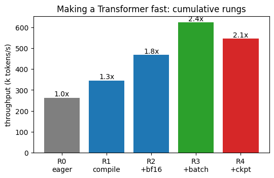
configurations = ['R0\nun-jitted', 'R1\njit', 'R2\n+bf16', 'R3\n+batch', 'R4\n+ckpt']
tputs = [tput0, tput1, tput2, tput3, tput4]
print(f'cumulative, R1 -> R3: {tputs[3] / tputs[1]:.2f}x '
      f'(and R0 -> R3: {tputs[3] / tputs[0]:.0f}x)')
d2l.plt.figure(figsize=(6, 3.5))
bars = d2l.plt.bar(configurations, [t / 1e3 for t in tputs],
                   color=['#7f7f7f', '#1f77b4', '#1f77b4', '#2ca02c', '#d62728'])
d2l.plt.ylabel('throughput (k tokens/s)')
d2l.plt.title('Making a Transformer fast: cumulative configurations')
for b, t in zip(bars, tputs):
    d2l.plt.text(b.get_x() + b.get_width() / 2, t / 1e3,
                 f'{t / tputs[1]:.2f}x', ha='center', va='bottom')
d2l.plt.show()
cumulative, R1 -> R3: 1.73x (and R0 -> R3: 32x)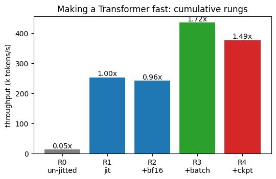
Compilation raises throughput by roughly 1.2 times by fusing the elementwise operations identified in the profile. Bf16 adds about another 50% once the matrices are wide enough to use tensor cores effectively. Increasing the batch adds roughly 1.2 times by raising arithmetic intensity. Checkpointing reduces throughput by about 10% while reducing peak memory from about 9 GiB to 3 GiB; memory capacity was not the limiting resource in this configuration. These single-window ratios vary by several percentage points on repetition. Their cumulative effect through the larger-batch configuration is a little over two times on this host. The result supports an iterative procedure: profile the current configuration, change the identified limiting resource, verify correctness, and measure again.
Whole-step JIT raises throughput by roughly twenty times relative to the un-jitted diagnostic, which is why the jitted step is the practical baseline. Bf16 alone changes little at batch 64 because fixed per-step dispatch remains limiting. At batch 512, bf16 and the larger batch interact: neither isolated change improves this stack, while together they raise throughput by most of a factor of two. Checkpointing reduces throughput by about 10% while reducing planned temporary storage severalfold. From the jitted baseline through the larger-batch configuration, the cumulative increase is about 1.7 times on this host. The PyTorch and JAX sequences differ because their starting bottlenecks differ; both are selected by the same profile–change–verify procedure.
Throughput does not establish that the optimization preserves training behavior. We therefore train the final configuration — compiled, bf16, batch 512 — for a few hundred steps from a fresh initialization and watch the loss, smoothed over twenty steps, actually fall. (On this tiny corpus a few hundred big-batch steps revisit the text over a hundred times, so the loss falls very far — the assertion, not the final value, is the point.) Performance changes are valid only if the optimized model still trains:
learner = make_gpt()
learner_c = torch.compile(learner)
opt_l = torch.optim.AdamW(learner.parameters(), lr=1e-3)
losses = []
for _ in range(300):
    X, Y = next(big_stream)
    opt_l.zero_grad(set_to_none=True)
    with torch.autocast('cuda', dtype=torch.bfloat16):
        loss = F.cross_entropy(learner_c(X).reshape(-1, vocab_size),
                               Y.reshape(-1))
    loss.backward(); opt_l.step()
    losses.append(loss.detach())       # no host read in the hot loop (13.1)
losses = torch.stack(losses).cpu()
first, last = losses[:20].mean(), losses[-20:].mean()
print(f'smoothed loss: first 20 steps {first:.2f} -> last 20 steps {last:.2f}')
assert last < first, 'speed that breaks the model is not speed'
smoothed loss: first 20 steps 3.01 -> last 20 steps 0.07learner = make_bf16_gpt()
opt_l = nnx.Optimizer(learner, optax.adamw(1e-3), wrt=nnx.Param)
losses = []
for _ in range(300):
X, Y = next(big_stream)
losses.append(step_bf16(learner, opt_l, X, Y)) # no host read (13.1)
losses = jnp.stack(losses)
first, last = losses[:20].mean(), losses[-20:].mean()
print(f'smoothed loss: first 20 steps {first:.2f} -> last 20 steps {last:.2f}')
assert last < first, 'speed that breaks the model is not speed'smoothed loss: first 20 steps 2.84 -> last 20 steps 0.0613.7.5 Further Optimization Techniques
The competitive edge of this method is a spectator sport. The modded-nanoGPT speedrun tracks the wall-clock time to train a small GPT to a target loss, and its record holders read like this chapter’s table of contents stacked to the ceiling: compiled and fused kernels (Section 13.3), block-sparse and FlashAttention variants (Section 10.5), a better optimizer (Section 9.9), aggressive low precision down to fp8 — each record a new configuration on a cumulative comparison like ours. fp8 tensor cores exist on our Ada GPUs, but the recipe for training in fp8 (its own loss-scaling and master-copy discipline) is deferred to the Language Models part, along with the multi-node parallelism where these techniques are stacked at frontier scale.
That is where the chapter ends, seven sections deep into a single idea. The machine has two budgets, arithmetic and bandwidth; a program lives in one of three regimes; and the way to make anything fast is always the same loop — measure, classify, fix, re-measure — now demonstrated on a real model, one configuration at a time.
13.7.6 Summary
- We profiled a baseline, classified its limiting regime, applied one technique, and profiled again. On the GPT of Section 11.2 (width 512, about 19 million parameters), compilation improved throughput by roughly 1.2×. Bf16 and a larger batch supplied further gains, for a cumulative improvement of a little over 2× in this experiment.
- Every configuration is attributed to a section, and the bottleneck is re-profiled as it moves: after compilation the elementwise tail is fused away and the matmuls’ share rises, which is what makes precision the next fix.
- Measurement is a technique too, and it can fail: a ragged final batch put a
torch.compileretrace inside our timing window, and the profiler’s instrumentation outlived its cell until told otherwise. Both had to be fixed before the cumulative comparison meant anything. - Two configurations teach by not helping: bf16 is a negative configuration at width 256 (matmuls too small for the tensor cores), and activation checkpointing is a negative configuration here (memory is not the binding constraint). Knowing when a technique does not apply is the method too.
- Data parallelism is predicted before it is measured: a transformer’s parameters scale with its compute, so DP on our host-staged fabric is communication-hungry — the measured throughput lands at the cost model’s no-overlap floor (a shade above it at two GPUs, a shade below at four, where the host-staged fabric no longer sustains its two-GPU bandwidth), nowhere near the linear ceiling. The prediction-then-measurement is the demonstration.
- The same procedure uses the compiler’s cost accounting in JAX. On the GPT of Section 11.2, JIT compilation improves throughput by about twenty times over un-jitted execution. Bf16 at batch 64 has little effect, and increasing the fp32 batch alone reduces throughput; together, reduced precision and the larger batch improve throughput by most of a factor of two over the jitted baseline.
- Precision in JAX is explicit, and layered: casting the arrays is not enough — flax modules remember a compute dtype from construction, and the model’s own fp32 arithmetic (rope’s trigonometry) promotes values straight back, which the attention kernel refuses loudly. The naive cast measured exactly like fp32; one dtype print exposed it. The masters, the gradients, and the Adam state stay fp32 by construction.
- Measurement is a technique too, and it can fail: the stock
tf.dataloader silently taxed the fastest configurations (fixed by staging the 5 MB corpus on device), and re-timing one cached batch flatters throughput by double-digit percent. Both had to be fixed before the cumulative comparison meant anything. - Configurations that do not help teach the most: bf16 at batch 64 is a null configuration here — the wall was per-step dispatch, which precision cannot touch — and checkpointing costs time to save memory the compiler’s plan said we did not need. Knowing when a technique does not apply is the method too.
- Data parallelism is predicted before it is measured: with \(\beta\) from 13.5’s measured
psum, Equation 13.5.2 prices the \(k=2\) gain at roughly nothing — the measurement lands at or below that floor — and \(k=4\) falls well short of the floor as the host-staged fabric sags. Declarative sharding then makes rerunning the fast configuration a loop rather than a launcher, and its recovered efficiency is the cost model’s grown compute term, verified.
13.7.7 Exercises
Attribution under interaction. Suppose that four single-GPU configurations of the GPT of Section 13.7.1 reach the following throughputs, relative to the fp32 step at batch 64: the bf16 step at batch 64 reaches 1.03, the fp32 step at batch 512 reaches 0.85, and the bf16 step at batch 512 reaches 1.75. Let \(r_{p,b}\) denote the relative throughput at precision \(p\) and batch size \(b\).
A cumulative comparison applies bf16 first and the larger batch second. Compute the ratio that it attributes to each change. Repeat the computation for the opposite order.
Show that both orders attribute the same ratio to each change exactly when the interaction ratio
\[\frac{r_{\textrm{bf16},512}\; r_{\textrm{fp32},64}}{r_{\textrm{bf16},64}\; r_{\textrm{fp32},512}} \tag{13.7.1}\]
equals 1, and evaluate it for the numbers above.
A leave-one-out ablation credits each change with the ratio of the final configuration to the final configuration without that change. Show that the two leave-one-out credits do not multiply to the total ratio of 1.75, and that the geometric means of each change’s ratios over the two orders do.
[code] Model FLOPs utilization. The GPT of Section 13.7.1 has \(L = 6\) blocks of width \(d = 512\) and reads contexts of \(T = 128\) tokens. Up to the rounding of the SwiGLU width, each block holds \(12d^2\) weights in its matrix products, and training costs about 6 FLOPs per weight and token, forward and backward pass together.
- The scores \(\mathbf{Q}\mathbf{K}^\top\) and the weighted sum of the values are matrix products without weights. Count their training FLOPs per token and block, taking the backward pass as twice the forward pass and counting the masked scores. Show that their ratio to the weight FLOPs is \(T/(6d)\), and evaluate the ratio for this GPT and for a context of 1,024 tokens.
- Compute the training FLOPs per token and per step at batch 64. From
tput1andtput3of your run, compute the achieved TFLOP/s of Configuration 1 and Configuration 3 of Section 13.7.3, and the fraction of the dense peak of their format in Table 13.2.1 that each reaches. Take the tf32 peak as half the bf16 entry. - A utilization figure can count the FLOPs that the model requires or the FLOPs that the hardware executes. Name two features of the configurations in Section 13.7.3 for which the two counts differ, and state the direction of each difference.
Throughput versus time to target. The cumulative comparison of Section 13.7.4 ranks configurations by tokens per second, whereas the speedrun of Section 13.7.5 ranks them by the wall-clock time to a target loss. By Equation 9.10.3, training at batch size \(b\) needs \(E(b) = E_{\min}(1 + b/b_{\textrm{noise}})\) examples to reach the target.
Let \(\rho > 1\) be the ratio of the throughput at batch 512 to the throughput at batch 64. Show that batch 512 reaches the target sooner exactly when
\[b_{\textrm{noise}} > \frac{512 - 64\rho}{\rho - 1}, \tag{13.7.2}\]
and evaluate the threshold for \(\rho = 1.2\) and for \(\rho = 1.7\).
Classify each configuration of Section 13.7.3, including Configuration 5 under weak scaling, and the switch to the optimizer of Section 9.9 in the speedrun, by whether it changes \(E(b)\), the throughput, or both.
[code] Fixed cost per step. ● Model the time of one training step at batch size \(B\) as
\[t(B) = t_0 + c\,B, \tag{13.7.3}\]
where \(t_0\) is a cost per step that does not depend on the batch and \(c\) is the cost per sequence.
- Measure the step time of Configuration 1 and of Configuration 2 of Section 13.7.3 with
throughputfor \(B \in \{16, 32, 64, 128, 256\}\), and fit \(t_0\) and \(c\) to each configuration by least squares. - Compare the fitted \(t_0\) and \(c\) of the two configurations, and explain each difference by the work that bf16 changes per step and per sequence. Use the fits to predict the throughput ratio of the two configurations at batch 64 and at batch 512, and compare the bf16 prediction at batch 512 with
tput3. - Find the batch at which \(t_0\) is a tenth of the bf16 step time. Configuration 4 costs about a tenth of the throughput of Configuration 3. From the memory that Configurations 3 and 4 report, estimate the largest bf16 batch that fits on the card with and without checkpointing. Use the bf16 fit to decide whether the larger batch that checkpointing admits repays that cost.
- Measure the step time of Configuration 1 and of Configuration 2 of Section 13.7.3 with
[code] Noise floor. Each throughput in Section 13.7.4 comes from a single timed window.
- Call
throughputten times in a row for Configuration 1 of Section 13.7.3, and report the mean and the relative standard deviation of the ten results. - Estimate the ratio of Configuration 2 to Configuration 1 twice: from two blocks of ten consecutive windows, and from ten pairs of alternating windows. Suppose that the GPU clock drifts slowly during the measurement. Explain which of the two designs cancels the drift, and compare the two estimates.
- Suppose that windows vary independently with the relative standard deviation of the first sub-problem. Find the number of windows per configuration that resolves a change of 3% at two standard errors of the ratio. Which ratios between neighboring bars of Section 13.7.4 does one window per configuration resolve?
- Call
[code] Causality gate. The training run at the end of Section 13.7.4 accepts the final configuration when the smoothed loss falls. Consider an optimized attention kernel that silently ignores the causal mask.
- Predict how the training loss of the GPT behaves with this kernel, and whether the assertion
last < firstpasses. Explain why the loss on the validation windows ofd2l.TimeMachinedoes not detect the defect either. - Write a gate that changes the last input token of every sequence in a batch and compares the logits at all earlier positions before and after the change. Run it on
learnerand on a copy ofd2l.GPTwhose attention omits the mask, and justify the tolerance that you choose.
- Predict how the training loss of the GPT behaves with this kernel, and whether the assertion
[extended] Another model. ● Apply the method of this section to
MambaLMof Section 12.3.3.1 or tod2l.ViTof- Write a benchmark contract in the form of the table in Section 13.7.1, profile the baseline, and classify its limiting regime in the terms of Section 13.1.4 before choosing the first change.
- Apply compilation, bf16, a larger batch, and activation checkpointing one at a time, with a correctness check before every timing, and plot the cumulative comparison.
- Identify every configuration whose effect changes sign relative to the GPT, and explain each change by the mechanism that the configuration targets.
[code] Retrace in the window. The stream
batchesdrops the final batch of every epoch, which has fewer rows than the others.- The training split holds 10,000 windows. Compute the number of batches per epoch at batch 64 and the size of the last batch. On a fresh stream without the filter, at which step does the first short batch arrive, and does it fall into the 60 warm-up steps or into the 100 timed steps of
throughput? - Remove the condition
X.shape[0] == dm.batch_sizefrombatches. Calltorch._dynamo.reset(), so that no graph compiled earlier for another batch size remains, turn ontorch._logging.set_logs(recompiles=True), and measure Configuration 1 of Section 13.7.3 on a fresh stream. Compare the throughput withtput1, and relate the difference to the recompilation that the log reports. - Time a second window that contains the short batch of the next epoch. Compare its throughput with the first window and with
tput1, and explain both comparisons from the log.
- The training split holds 10,000 windows. Compute the number of batches per epoch at batch 64 and the size of the last batch. On a fresh stream without the filter, at which step does the first short batch arrive, and does it fall into the 60 warm-up steps or into the 100 timed steps of
[code] bf16 at width 256. ● At
num_hiddens=256, Section 13.7.1 reports that bf16 slows the compiled step down.- Consider the product of the \(8192 \times 256\) activations of one batch with a \(256 \times 256\) weight matrix, the shape of the output projection \(\mathbf{W}_o\). Compute its arithmetic intensity with 4-byte tf32 operands and with 2-byte bf16 operands, place both on the roofline of Figure 13.1.1 for the RTX 4090, taking the tf32 peak as half the bf16 peak, and predict the speedup of bf16 for this product.
- Run the baseline and Configurations 1 and 2 of Section 13.7.3 at
num_hiddens=256. Profile Configurations 1 and 2 withprofile_top, and split the device time of each between the matrix products and all other kernels. Account for the measured ratio of Configuration 2 to Configuration 1 kernel by kernel, and compare it with the prediction.
[code] Attention kernel.
d2l.GPTcomputes attention withF.scaled_dot_product_attention, which selects a fused kernel when its inputs allow one.- For a batch of \(B\) sequences of \(T\) tokens and 8 heads, compute the bytes of the score matrices of one layer at \(B = 64, T = 128\) and at \(B = 8, T = 1024\), two shapes with the same number of tokens. Count 4 bytes per score, because the attention that writes the scores to memory forms them and their softmax in fp32 even for bf16 inputs. Show that at a fixed number of tokens per step these bytes grow in proportion to \(T\).
- Write a bf16 step that calls the uncompiled
modelunder autocast. Measure tokens/s andtorch.cuda.max_memory_allocatedat both shapes, once with the default backend and once insidesdpa_kernel(SDPBackend.MATH)fromtorch.nn.attention, which writes the scores to memory. Relate the four results to the first sub-problem.
[code] Parity tolerance. Configuration 1 of Section 13.7.3 asserts that
compiled(X)andmodel(X)agree withinatol=1e-2, and attributes the residue to tf32 matrix products whose summation order the fusion changes.- Measure the largest absolute difference between
compiled(X)andmodel(X)undertorch.set_float32_matmul_precision('high')and under'highest', callingtorch._dynamo.reset()before the compiled model runs again. Measure also the difference betweenmodel(X)under the two settings. State what the three numbers imply for the attribution. - Measure the largest difference in the check of Configuration 4 between
ckpt_gpt(X)andmodel(X), and explain why that check can useatol=1e-6.
- Measure the largest absolute difference between
[code] Data-parallel overlap. ● Let \(\phi\) be the fraction of \(t_{\text{comm}}\) that DDP hides under the backward pass, so that a step on \(k\) GPUs takes
\[t_{\text{step}} = t_{\text{compute}} + (1 - \phi)\, t_{\text{comm}}. \tag{13.7.4}\]
- Compute \(\phi\) at \(k = 2\) and \(k = 4\) from the measured tokens/s of Configuration 5 of Section 13.7.3 and the \(t_{\text{comm}}\) and \(t_{\text{compute}}\) that it prints. What does a negative value of \(\phi\) indicate?
- Modify
GPT_DDPso that every rank runs the compiled bf16 step at batch 512 on batches of constant shape. Before launching it, predict the no-overlap floor at \(k = 2\) and \(k = 4\) fromtput3and Equation 13.5.2. - Measure tokens/s at \(k = 2\) and \(k = 4\) with
ddp_gpt_tokens. Compute the weak-scaling efficiency againsttput3and the value of \(\phi\), and explain the change from Configuration 5 by the terms of Equation 13.5.2.
[code] Retrace in the window. The stream
batchesrounds every epoch down to whole batches.- The training split holds 10,000 windows. Compute the number of batches per epoch at batch 64 and the size of the last batch if the epoch were not rounded. On a fresh stream without the rounding, at which step does the first short batch arrive, and does it fall into the 60 warm-up steps or into the 100 timed steps of
throughput? - Replace
n = (len(X) // B) * Binbatchesbyn = len(X). Calljax.clear_caches(), so that no program compiled earlier for another batch size remains, turn onjax.config.update('jax_log_compiles', True), and measure Configuration 1 of Section 13.7.3 on a fresh stream. Compare the throughput withtput1, and relate the difference to the compilation that the log reports. - Time a second window that contains the short batch of the next epoch. Compare its throughput with the first window and with
tput1, and explain both comparisons from the log.
- The training split holds 10,000 windows. Compute the number of batches per epoch at batch 64 and the size of the last batch if the epoch were not rounded. On a fresh stream without the rounding, at which step does the first short batch arrive, and does it fall into the 60 warm-up steps or into the 100 timed steps of
[code] Precision audit. The receipts of Configuration 2 in Section 13.7.3 check the dtype of one layer’s output. An audit of the lowered program checks every matrix product of the step.
- Write a function that lowers a jitted step with
.lower(...), reads its StableHLO with.as_text(), and counts thestablehlo.dot_generaloperations by the dtypes of their operands. Apply it tostep_jit,step_naive, andstep_bf16. - Locate the
stablehlo.convertoperations through which the fp32 gradients ofstep_bf16arise, and name the forward operation whose transpose each of them is.
- Write a function that lowers a jitted step with
[code] Attention kernel. ●
d2l.GPTcallsjax.nn.dot_product_attentionwithout naming an implementation, and the default lowering writes the score matrices to memory. The fused kernel of Section 10.5 is selected byimplementation='cudnn'and accepts only half-precision inputs.- For a batch of \(B\) sequences of \(T\) tokens and 8 heads, compute the bytes of the score matrices of one layer at \(B = 64, T = 128\) and at \(B = 8, T = 1024\), two shapes with the same number of tokens. Count 4 bytes per score, because the attention that writes the scores to memory forms them and their softmax in fp32 even for bf16 inputs. Show that at a fixed number of tokens per step these bytes grow in proportion to \(T\).
- Subclass
Bf16GPT.CausalAttentionso that it names the cuDNN implementation, and verify that its logits agree with those ofBf16GPT. - Measure tokens/s and the planned temporary bytes of
memory_analysis()for the bf16 step at both shapes and with both attention implementations. Relate the four results to the first sub-problem.
[code] Parity tolerance. Configuration 1 of Section 13.7.3 asserts that
fwd(model, X)andmodel(X)agree withinatol=1e-2, and attributes the residue of a few times \(10^{-4}\) to tf32 arithmetic whose summation order the fusion changes.- Measure the largest absolute difference between
fwd(model, X)andmodel(X)under the default precision and insidewith jax.default_matmul_precision('float32'):. Measure also the difference betweenmodel(X)under the two settings. State what the three numbers imply for the attribution. - Measure the largest difference in the check of Configuration 4 between
ckpt_forward(half, Xb)andhalf(Xb), and explain why that check can useatol=1e-6.
- Measure the largest absolute difference between
[code] Data-parallel overlap. ● Let \(\phi\) be the fraction of \(t_{\text{comm}}\) that the compiled step hides under computation, so that a step on \(k\) GPUs takes
\[t_{\text{step}} = t_{\text{compute}} + (1 - \phi)\, t_{\text{comm}}. \tag{13.7.5}\]
- Compute \(\phi\) at \(k = 2\) and \(k = 4\) from the measured tokens/s of Configuration 5 of Section 13.7.3 and the \(t_{\text{comm}}\) and \(t_{\text{compute}}\) that it prints. What does a negative value of \(\phi\) indicate?
- The data-parallel run of
step_bf16throughdp_tokensat a per-device batch of 512 prints its weak-scaling efficiency. Predict its no-overlap floor at \(k = 2\) and \(k = 4\) fromtput3,n_bytes, andbeta, and compute \(\phi\) from the printed efficiency. - Repeat that run with per-device batches of 128 and 256, measure the single-GPU throughput of
step_bf16at each batch, and plot the weak-scaling efficiency and \(\phi\) against the per-device batch. Explain the trend by the terms of Equation 13.5.2.
[code] Sharded parameters. ● Configuration 5 of Section 13.7.3 replicates the model and the optimizer state on every device and shards only the batch.
- Change
dp_setupso that every array of the model and optimizer state is sharded over the'data'mesh axis along its first axis whose length is divisible by \(k\), and stays replicated when no axis is. Leavetrain_stepunchanged. Check the layout of one weight matrix withjax.debug.visualize_array_sharding. - Compile
step_jiton the sharded state and list the collective operations in.as_text()of the compiled step with their sizes. Decide whether the step gathers each weight once or twice, and compare its bytes per device with the allreduce of Equation 13.5.1. - Measure tokens/s at \(k = 2\) and \(k = 4\), and compare them with Configuration 5. Compute from Section 13.4.1 the memory per device that sharding saves for this GPT at \(k = 4\). Find the parameter count at which this saving equals
plan16_gib, the planned temporary memory ofstep_bf16at batch 512, and explain what this count implies about the model sizes for which sharding the state pays on 24-GB cards.
- Change