import torch1.1 Data Manipulation
Deep learning programs store numerical data in \(n\)-dimensional arrays, which we call tensors. A tensor may represent a single measurement, a feature vector, an image, or a batch of examples. This section introduces the operations needed to create, inspect, and manipulate these arrays. If you already know the NumPy scientific computing package (Harris et al. 2020), much of this will look familiar. For all modern deep learning frameworks, the tensor class (ndarray in MXNet, Tensor in PyTorch and TensorFlow, jax.Array in JAX) resembles NumPy’s ndarray, with two additions. First, the tensor class supports automatic differentiation (Section 1.5). Second, it uses GPUs to accelerate numerical computation, whereas NumPy only runs on CPUs. These properties support both gradient-based learning and accelerated numerical computation. (We cover how to place tensors on a GPU and move them between devices in Section 5.7; until then, every tensor we create lives in CPU memory.)
1.1.1 Getting Started
To start, we import the PyTorch library. The package name is torch.
To start, we import tensorflow. For brevity, practitioners often assign the alias tf.
To start, we import jax and its NumPy-like numerical interface jax.numpy, conventionally aliased as jnp.
To start, we import the np (numpy) and npx (numpy_extension) modules from MXNet. Here, the np module includes functions supported by NumPy, while the npx module contains a set of extensions that support deep learning within a NumPy-like environment. When using tensors, we almost always invoke the set_np function: this is for compatibility of tensor processing by other components of MXNet.
import tensorflow as tfimport jax
from jax import numpy as jnpfrom mxnet import np, npx
npx.set_np()A tensor represents a (possibly multidimensional) array of numerical values. In the one-dimensional case, i.e., when only one axis is needed for the data, a tensor is called a vector. With two axes, a tensor is called a matrix. With \(k > 2\) axes, we drop the specialized names and refer to the object as a \(k^\textrm{th}\)-order tensor.
Several functions create new tensors prepopulated with values. For example, by invoking arange(n), we can create a vector of evenly spaced values, starting at 0 (included) and ending at n (not included). By default, the interval size is \(1\). Unless otherwise specified, new tensors are stored in main memory and designated for CPU-based computation.
In TensorFlow, this function is named range rather than arange.
x = torch.arange(12, dtype=torch.float32)
x
tensor([ 0., 1., 2., 3., 4., 5., 6., 7., 8., 9., 10., 11.])x = tf.range(12, dtype=tf.float32)
x<tf.Tensor: shape=(12,), dtype=float32, numpy=
array([ 0., 1., 2., 3., 4., 5., 6., 7., 8., 9., 10., 11.],
dtype=float32)>x = jnp.arange(12, dtype=jnp.float32)
xArray([ 0., 1., 2., 3., 4., 5., 6., 7., 8., 9., 10., 11.], dtype=float32)x = np.arange(12)
xarray([ 0., 1., 2., 3., 4., 5., 6., 7., 8., 9., 10., 11.])The dtype (data type) of a tensor determines how its elements are stored. We use 32-bit floating point (float32) as the default throughout these chapters. Training systems also use lower-precision floating-point formats, often together with higher-precision accumulation. Section 5.5 develops those formats and their numerical tradeoffs. You can inspect a tensor’s type via its dtype attribute. In finite precision, naive computations can overflow or underflow, which is why later sections compute quantities such as the softmax and cross-entropy with stabilized formulas (Section 3.1).
Integer ranges like arange default to an integer type, which is why the cell above requests dtype=torch.float32 explicitly. To cast between types, use .to (or shortcuts such as .float()).
Integer ranges like range default to an integer type, which is why the cell above requests dtype=tf.float32 explicitly. To cast between types, use tf.cast.
Integer ranges like arange default to an integer type, which is why the cell above requests dtype=jnp.float32 explicitly. To cast between types, use astype.
MXNet’s np.arange already defaults to float32, so the cell above needs no explicit dtype. To cast between types, use astype.
x.numel()12tf.size(x)<tf.Tensor: shape=(), dtype=int32, numpy=12>x.size12x.size12We can access a tensor’s shape (the length along each axis) by inspecting its shape attribute. Because we are dealing with a vector here, the shape contains a single element and is identical to the size.
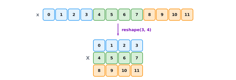
x.shapetorch.Size([12])TensorShape([12])(12,)(12,)We can change the shape of a tensor without altering its size or values, by invoking reshape. For example, we can transform our vector x whose shape is (12,) to a matrix X with shape (3, 4). This new tensor retains all elements but reconfigures them into a matrix. The elements of our vector are laid out one row at a time and thus x[3] == X[0, 3], as Figure 1.1.1 illustrates.
X = x.reshape(3, 4)
X
tensor([[ 0., 1., 2., 3.],
[ 4., 5., 6., 7.],
[ 8., 9., 10., 11.]])X = tf.reshape(x, (3, 4))
X<tf.Tensor: shape=(3, 4), dtype=float32, numpy=
array([[ 0., 1., 2., 3.],
[ 4., 5., 6., 7.],
[ 8., 9., 10., 11.]], dtype=float32)>X = x.reshape(3, 4)
XArray([[ 0., 1., 2., 3.],
[ 4., 5., 6., 7.],
[ 8., 9., 10., 11.]], dtype=float32)X = x.reshape(3, 4)
Xarray([[ 0., 1., 2., 3.],
[ 4., 5., 6., 7.],
[ 8., 9., 10., 11.]])Specifying every shape component to reshape is redundant. Because we already know our tensor’s size, we can work out one component of the shape given the rest. For example, given a tensor of size \(n\) and target shape (\(h\), \(w\)), we know that \(w = n/h\). To automatically infer one component of the shape, we can place a -1 for the shape component that should be inferred automatically. In our case, instead of calling x.reshape(3, 4), we could have equivalently called x.reshape(-1, 4) or x.reshape(3, -1).
For a contiguous tensor such as x, a framework can implement reshape by changing only shape metadata. More generally, reshape may return either a view that shares storage or a copy, depending on the layout and framework. Code should therefore not rely on storage sharing unless it explicitly asks for a view and satisfies that operation’s layout requirements.
Practitioners often need to work with tensors initialized to contain all 0s or 1s. We can construct a tensor with all elements set to 0 and a shape of (2, 3, 4) via the zeros function.
torch.zeros((2, 3, 4))tensor([[[0., 0., 0., 0.],
[0., 0., 0., 0.],
[0., 0., 0., 0.]],
[[0., 0., 0., 0.],
[0., 0., 0., 0.],
[0., 0., 0., 0.]]])tf.zeros((2, 3, 4))<tf.Tensor: shape=(2, 3, 4), dtype=float32, numpy=
array([[[0., 0., 0., 0.],
[0., 0., 0., 0.],
[0., 0., 0., 0.]],
[[0., 0., 0., 0.],
[0., 0., 0., 0.],
[0., 0., 0., 0.]]], dtype=float32)>jnp.zeros((2, 3, 4))Array([[[0., 0., 0., 0.],
[0., 0., 0., 0.],
[0., 0., 0., 0.]],
[[0., 0., 0., 0.],
[0., 0., 0., 0.],
[0., 0., 0., 0.]]], dtype=float32)np.zeros((2, 3, 4))array([[[0., 0., 0., 0.],
[0., 0., 0., 0.],
[0., 0., 0., 0.]],
[[0., 0., 0., 0.],
[0., 0., 0., 0.],
[0., 0., 0., 0.]]])Similarly, we can create a tensor with all 1s by invoking ones.
torch.ones((2, 3, 4))tensor([[[1., 1., 1., 1.],
[1., 1., 1., 1.],
[1., 1., 1., 1.]],
[[1., 1., 1., 1.],
[1., 1., 1., 1.],
[1., 1., 1., 1.]]])tf.ones((2, 3, 4))<tf.Tensor: shape=(2, 3, 4), dtype=float32, numpy=
array([[[1., 1., 1., 1.],
[1., 1., 1., 1.],
[1., 1., 1., 1.]],
[[1., 1., 1., 1.],
[1., 1., 1., 1.],
[1., 1., 1., 1.]]], dtype=float32)>jnp.ones((2, 3, 4))Array([[[1., 1., 1., 1.],
[1., 1., 1., 1.],
[1., 1., 1., 1.]],
[[1., 1., 1., 1.],
[1., 1., 1., 1.],
[1., 1., 1., 1.]]], dtype=float32)np.ones((2, 3, 4))array([[[1., 1., 1., 1.],
[1., 1., 1., 1.],
[1., 1., 1., 1.]],
[[1., 1., 1., 1.],
[1., 1., 1., 1.],
[1., 1., 1., 1.]]])We often wish to sample each element randomly (and independently) from a given probability distribution. For example, the parameters of neural networks are often initialized randomly, in part to break symmetry between units: if every weight in a layer started at the same value (say, zero), the units would all compute the same thing and could never specialize. The following snippet creates a tensor with elements drawn from a standard Gaussian (normal) distribution with mean 0 and standard deviation 1.
torch.randn(3, 4)tensor([[ 0.0760, 0.9297, 1.0870, -0.4283],
[ 0.4409, -0.2029, -0.0518, 0.6283],
[ 0.6729, 0.7885, -1.2366, 1.3750]])tf.random.normal(shape=[3, 4])<tf.Tensor: shape=(3, 4), dtype=float32, numpy=
array([[ 0.5056444 , -0.5161691 , -0.42710906, 0.35468888],
[ 1.6351061 , -0.82661825, -1.6055739 , 0.2748962 ],
[-1.1734169 , 1.2975142 , 0.28410774, 2.0338938 ]],
dtype=float32)># Any call of a random function in JAX requires a key to be
# specified, feeding the same key to a random function will
# always result in the same sample being generated
jax.random.normal(jax.random.key(0), (3, 4))Array([[ 1.6226422 , 2.0252647 , -0.43359444, -0.07861735],
[ 0.1760909 , -0.97208923, -0.49529874, 0.4943786 ],
[ 0.6643493 , -0.9501635 , 2.1795304 , -1.9551506 ]], dtype=float32)np.random.normal(0, 1, size=(3, 4))array([[ 1.1791748 , -0.69516647, 0.7244036 , 0.07209436],
[ 1.2696365 , -0.05372444, -1.4317043 , -0.4031657 ],
[-0.11129929, -1.4493049 , 2.1092663 , -2.345926 ]])Random sampling raises the question of reproducibility. Calling a sampler repeatedly gives different draws, which is usually what we want, but for debugging or for figures that should not change between runs we fix a seed.
PyTorch keeps a global generator that torch.manual_seed resets: after seeding, the sequence of draws is repeatable.
TensorFlow keeps a global generator that tf.random.set_seed resets: after seeding, the sequence of draws is repeatable.
JAX takes a more explicit stance: instead of a hidden global generator, every draw threads a key through the sampler, and the same key always yields the same sample, as the cell above shows.
MXNet keeps a global generator that np.random.seed resets: after seeding, the sequence of draws is repeatable.
Finally, we can construct tensors by supplying the exact values for each element via (possibly nested) Python list(s) containing numerical literals. Here, we construct a matrix with a list of lists, where the outermost list corresponds to axis 0, and the inner list corresponds to axis 1.
torch.tensor([[2, 1, 4, 3], [1, 2, 3, 4], [4, 3, 2, 1]])tensor([[2, 1, 4, 3],
[1, 2, 3, 4],
[4, 3, 2, 1]])tf.constant([[2, 1, 4, 3], [1, 2, 3, 4], [4, 3, 2, 1]])<tf.Tensor: shape=(3, 4), dtype=int32, numpy=
array([[2, 1, 4, 3],
[1, 2, 3, 4],
[4, 3, 2, 1]], dtype=int32)>jnp.array([[2, 1, 4, 3], [1, 2, 3, 4], [4, 3, 2, 1]])Array([[2, 1, 4, 3],
[1, 2, 3, 4],
[4, 3, 2, 1]], dtype=int32)np.array([[2, 1, 4, 3], [1, 2, 3, 4], [4, 3, 2, 1]])array([[2., 1., 4., 3.],
[1., 2., 3., 4.],
[4., 3., 2., 1.]])1.1.2 Indexing and Slicing
As with Python lists, we can access tensor elements by indexing (starting with 0). To access an element based on its position relative to the end of the list, we can use negative indexing. We can also access whole ranges of indices via slicing (e.g., X[start:stop]), where the returned value includes the first index (start) but not the last (stop). Finally, when only one index (or slice) is specified for a \(k^\textrm{th}\)-order tensor, it is applied along axis 0. Thus, in the following code, [-1] selects the last row and [1:3] selects the second and third rows.
X[-1], X[1:3](tensor([ 8., 9., 10., 11.]),
tensor([[ 4., 5., 6., 7.],
[ 8., 9., 10., 11.]]))(<tf.Tensor: shape=(4,), dtype=float32, numpy=array([ 8., 9., 10., 11.], dtype=float32)>,
<tf.Tensor: shape=(2, 4), dtype=float32, numpy=
array([[ 4., 5., 6., 7.],
[ 8., 9., 10., 11.]], dtype=float32)>)(Array([ 8., 9., 10., 11.], dtype=float32),
Array([[ 4., 5., 6., 7.],
[ 8., 9., 10., 11.]], dtype=float32))(array([ 8., 9., 10., 11.]),
array([[ 4., 5., 6., 7.],
[ 8., 9., 10., 11.]]))Beyond reading them, we can also write elements of a matrix by specifying indices.
Tensors in TensorFlow are immutable, and cannot be assigned to. Variables in TensorFlow are mutable containers of state that support assignments. Gradients in TensorFlow do not flow backward through Variable assignments.
Beyond assigning a value to the entire Variable, we can write elements of a Variable by specifying indices.
Beyond reading them, we can also write elements of a matrix by specifying indices.
X[1, 2] = 17
X
tensor([[ 0., 1., 2., 3.],
[ 4., 5., 17., 7.],
[ 8., 9., 10., 11.]])X_var = tf.Variable(X)
X_var[1, 2].assign(17)
X_var<tf.Variable 'Variable:0' shape=(3, 4) dtype=float32, numpy=
array([[ 0., 1., 2., 3.],
[ 4., 5., 17., 7.],
[ 8., 9., 10., 11.]], dtype=float32)># JAX arrays are immutable. jax.numpy.ndarray.at index
# update operators create a new array with the corresponding
# modifications made
X_new_1 = X.at[1, 2].set(17)
X_new_1Array([[ 0., 1., 2., 3.],
[ 4., 5., 17., 7.],
[ 8., 9., 10., 11.]], dtype=float32)X[1, 2] = 17
Xarray([[ 0., 1., 2., 3.],
[ 4., 5., 17., 7.],
[ 8., 9., 10., 11.]])If we want to assign multiple elements the same value, we apply the indexing on the left-hand side of the assignment operation. For instance, [:2, :] accesses the first and second rows, where : takes all the elements along axis 1 (column). While we discussed indexing for matrices, this also works for vectors and for tensors of more than two dimensions.
X[:2, :] = 12
X
tensor([[12., 12., 12., 12.],
[12., 12., 12., 12.],
[ 8., 9., 10., 11.]])X_var = tf.Variable(X)
X_var[:2, :].assign(tf.ones(X_var[:2,:].shape, dtype=tf.float32) * 12)
X_var<tf.Variable 'Variable:0' shape=(3, 4) dtype=float32, numpy=
array([[12., 12., 12., 12.],
[12., 12., 12., 12.],
[ 8., 9., 10., 11.]], dtype=float32)>X_new_2 = X_new_1.at[:2, :].set(12)
X_new_2Array([[12., 12., 12., 12.],
[12., 12., 12., 12.],
[ 8., 9., 10., 11.]], dtype=float32)X[:2, :] = 12
Xarray([[12., 12., 12., 12.],
[12., 12., 12., 12.],
[ 8., 9., 10., 11.]])1.1.3 Operations
Now that we know how to construct tensors and how to read from and write to their elements, we can begin to manipulate them with various mathematical operations. Among the most useful of these are the elementwise operations. These apply a standard scalar operation to each element of a tensor. For functions that take two tensors as inputs, elementwise operations apply some standard binary operator on each pair of corresponding elements. We can create an elementwise function from any function that maps from a scalar to a scalar.
In mathematical notation, we denote such unary scalar operators (taking one input) by the signature \(f: \mathbb{R} \rightarrow \mathbb{R}\). This means that the function maps from any real number onto some other real number. Most standard operators, including unary ones like \(e^x\), can be applied elementwise.
torch.exp(x)tensor([162754.7969, 162754.7969, 162754.7969, 162754.7969, 162754.7969,
162754.7969, 162754.7969, 162754.7969, 2980.9580, 8103.0840,
22026.4648, 59874.1406])tf.exp(x)<tf.Tensor: shape=(12,), dtype=float32, numpy=
array([1.0000000e+00, 2.7182817e+00, 7.3890562e+00, 2.0085537e+01,
5.4598148e+01, 1.4841316e+02, 4.0342880e+02, 1.0966332e+03,
2.9809580e+03, 8.1030840e+03, 2.2026467e+04, 5.9874145e+04],
dtype=float32)>jnp.exp(x)Array([1.0000000e+00, 2.7182817e+00, 7.3890562e+00, 2.0085537e+01,
5.4598148e+01, 1.4841316e+02, 4.0342880e+02, 1.0966332e+03,
2.9809580e+03, 8.1030840e+03, 2.2026467e+04, 5.9874145e+04], dtype=float32)np.exp(x)array([1.0000000e+00, 2.7182820e+00, 7.3890557e+00, 2.0085537e+01,
5.4598145e+01, 1.4841315e+02, 4.0342877e+02, 1.0966331e+03,
2.9809583e+03, 8.1030840e+03, 2.2026467e+04, 5.9874137e+04])Likewise, we denote binary scalar operators, which map pairs of real numbers to a (single) real number via the signature \(f: \mathbb{R}, \mathbb{R} \rightarrow \mathbb{R}\). Given any two vectors \(\mathbf{u}\) and \(\mathbf{v}\) of the same shape, and a binary operator \(f\), we can produce a vector \(\mathbf{c} = F(\mathbf{u},\mathbf{v})\) by setting \(c_i \gets f(u_i, v_i)\) for all \(i\), where \(c_i, u_i\), and \(v_i\) are the \(i^\textrm{th}\) elements of vectors \(\mathbf{c}, \mathbf{u}\), and \(\mathbf{v}\). Here, we produced the vector-valued \(F: \mathbb{R}^d, \mathbb{R}^d \rightarrow \mathbb{R}^d\) by lifting the scalar function to an elementwise vector operation. The common standard arithmetic operators for addition (+), subtraction (-), multiplication (*), division (/), and exponentiation (**) have all been lifted to elementwise operations for identically-shaped tensors of arbitrary shape.
x = torch.tensor([1.0, 2, 4, 8])
y = torch.tensor([2, 2, 2, 2])
x + y, x - y, x * y, x / y, x ** y
(tensor([ 3., 4., 6., 10.]),
tensor([-1., 0., 2., 6.]),
tensor([ 2., 4., 8., 16.]),
tensor([0.5000, 1.0000, 2.0000, 4.0000]),
tensor([ 1., 4., 16., 64.]))x = tf.constant([1.0, 2, 4, 8])
y = tf.constant([2.0, 2, 2, 2])
x + y, x - y, x * y, x / y, x ** y(<tf.Tensor: shape=(4,), dtype=float32, numpy=array([ 3., 4., 6., 10.], dtype=float32)>,
<tf.Tensor: shape=(4,), dtype=float32, numpy=array([-1., 0., 2., 6.], dtype=float32)>,
<tf.Tensor: shape=(4,), dtype=float32, numpy=array([ 2., 4., 8., 16.], dtype=float32)>,
<tf.Tensor: shape=(4,), dtype=float32, numpy=array([0.5, 1. , 2. , 4. ], dtype=float32)>,
<tf.Tensor: shape=(4,), dtype=float32, numpy=array([ 1., 4., 16., 64.], dtype=float32)>)x = jnp.array([1.0, 2, 4, 8])
y = jnp.array([2, 2, 2, 2])
x + y, x - y, x * y, x / y, x ** y(Array([ 3., 4., 6., 10.], dtype=float32),
Array([-1., 0., 2., 6.], dtype=float32),
Array([ 2., 4., 8., 16.], dtype=float32),
Array([0.5, 1. , 2. , 4. ], dtype=float32),
Array([ 1., 4., 16., 64.], dtype=float32))x = np.array([1, 2, 4, 8])
y = np.array([2, 2, 2, 2])
x + y, x - y, x * y, x / y, x ** y(array([ 3., 4., 6., 10.]),
array([-1., 0., 2., 6.]),
array([ 2., 4., 8., 16.]),
array([0.5, 1. , 2. , 4. ]),
array([ 1., 4., 16., 64.]))In addition to elementwise computations, we can also perform linear algebraic operations, such as dot products and matrix multiplications. We will elaborate on these in Section 1.3.
We can also concatenate multiple tensors, stacking them end-to-end to form a larger one. We provide a list of tensors and tell the system along which axis to concatenate. The example below shows what happens when we concatenate two matrices along rows (axis 0) instead of columns (axis 1). We can see that the first output’s axis-0 length (\(6\)) is the sum of the two input tensors’ axis-0 lengths (\(3 + 3\)); while the second output’s axis-1 length (\(8\)) is the sum of the two input tensors’ axis-1 lengths (\(4 + 4\)).
X = torch.arange(12, dtype=torch.float32).reshape((3,4))
Y = torch.tensor([[2.0, 1, 4, 3], [1, 2, 3, 4], [4, 3, 2, 1]])
torch.cat((X, Y), dim=0), torch.cat((X, Y), dim=1)
(tensor([[ 0., 1., 2., 3.],
[ 4., 5., 6., 7.],
[ 8., 9., 10., 11.],
[ 2., 1., 4., 3.],
[ 1., 2., 3., 4.],
[ 4., 3., 2., 1.]]),
tensor([[ 0., 1., 2., 3., 2., 1., 4., 3.],
[ 4., 5., 6., 7., 1., 2., 3., 4.],
[ 8., 9., 10., 11., 4., 3., 2., 1.]]))X = tf.reshape(tf.range(12, dtype=tf.float32), (3, 4))
Y = tf.constant([[2.0, 1, 4, 3], [1, 2, 3, 4], [4, 3, 2, 1]])
tf.concat([X, Y], axis=0), tf.concat([X, Y], axis=1)(<tf.Tensor: shape=(6, 4), dtype=float32, numpy=
array([[ 0., 1., 2., 3.],
[ 4., 5., 6., 7.],
[ 8., 9., 10., 11.],
[ 2., 1., 4., 3.],
[ 1., 2., 3., 4.],
[ 4., 3., 2., 1.]], dtype=float32)>,
<tf.Tensor: shape=(3, 8), dtype=float32, numpy=
array([[ 0., 1., 2., 3., 2., 1., 4., 3.],
[ 4., 5., 6., 7., 1., 2., 3., 4.],
[ 8., 9., 10., 11., 4., 3., 2., 1.]], dtype=float32)>)X = jnp.arange(12, dtype=jnp.float32).reshape((3, 4))
Y = jnp.array([[2.0, 1, 4, 3], [1, 2, 3, 4], [4, 3, 2, 1]])
jnp.concatenate((X, Y), axis=0), jnp.concatenate((X, Y), axis=1)(Array([[ 0., 1., 2., 3.],
[ 4., 5., 6., 7.],
[ 8., 9., 10., 11.],
[ 2., 1., 4., 3.],
[ 1., 2., 3., 4.],
[ 4., 3., 2., 1.]], dtype=float32),
Array([[ 0., 1., 2., 3., 2., 1., 4., 3.],
[ 4., 5., 6., 7., 1., 2., 3., 4.],
[ 8., 9., 10., 11., 4., 3., 2., 1.]], dtype=float32))X = np.arange(12).reshape(3, 4)
Y = np.array([[2, 1, 4, 3], [1, 2, 3, 4], [4, 3, 2, 1]])
np.concatenate([X, Y], axis=0), np.concatenate([X, Y], axis=1)(array([[ 0., 1., 2., 3.],
[ 4., 5., 6., 7.],
[ 8., 9., 10., 11.],
[ 2., 1., 4., 3.],
[ 1., 2., 3., 4.],
[ 4., 3., 2., 1.]]),
array([[ 0., 1., 2., 3., 2., 1., 4., 3.],
[ 4., 5., 6., 7., 1., 2., 3., 4.],
[ 8., 9., 10., 11., 4., 3., 2., 1.]]))Sometimes, we want to construct a boolean tensor via logical statements. Take X == Y as an example. For each position i, j, if X[i, j] and Y[i, j] are equal, then the corresponding entry in the result is True, otherwise it is False. (Booleans behave as 1 and 0 in arithmetic, so summing such a mask counts the positions where the two tensors agree.)
X == Ytensor([[False, True, False, True],
[False, False, False, False],
[False, False, False, False]])<tf.Tensor: shape=(3, 4), dtype=bool, numpy=
array([[False,  True, False,  True],
       [False, False, False, False],
[False, False, False, False]])>Array([[False, True, False, True],
[False, False, False, False],
[False, False, False, False]], dtype=bool)array([[False, True, False, True],
[False, False, False, False],
[False, False, False, False]])Summing all the elements in the tensor yields a tensor with only one element.
X.sum()tensor(66.)tf.reduce_sum(X)<tf.Tensor: shape=(), dtype=float32, numpy=66.0>X.sum()Array(66., dtype=float32)X.sum()array(66.)1.1.4 Broadcasting
By now, you know how to perform elementwise binary operations on two tensors of the same shape. Under certain conditions, even when shapes differ, we can still perform elementwise binary operations by invoking the broadcasting mechanism (a convention inherited from NumPy).
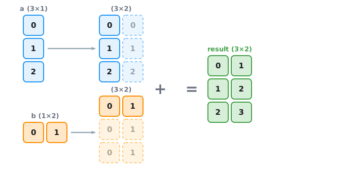
Broadcasting follows a simple rule. Line the two shapes up from the right and compare them axis by axis: two axes are compatible when they are equal or when one of them is \(1\) (a missing leading axis counts as \(1\)). The size-\(1\) axis is then stretched to match the other, by virtually copying its entries, and the elementwise operation is applied to the resulting arrays. If any pair of axes is incompatible, the operation raises an error rather than guessing. Figure 1.1.2 shows the mechanism at work on the example that follows: each size-\(1\) axis is stretched until both operands share the shape \(3\times2\).
a = torch.arange(3).reshape((3, 1))
b = torch.arange(2).reshape((1, 2))
a, b
(tensor([[0],
[1],
[2]]),
tensor([[0, 1]]))a = tf.reshape(tf.range(3), (3, 1))
b = tf.reshape(tf.range(2), (1, 2))
a, b(<tf.Tensor: shape=(3, 1), dtype=int32, numpy=
array([[0],
[1],
[2]], dtype=int32)>,
<tf.Tensor: shape=(1, 2), dtype=int32, numpy=array([[0, 1]], dtype=int32)>)a = jnp.arange(3).reshape((3, 1))
b = jnp.arange(2).reshape((1, 2))
a, b(Array([[0],
[1],
[2]], dtype=int32),
Array([[0, 1]], dtype=int32))a = np.arange(3).reshape(3, 1)
b = np.arange(2).reshape(1, 2)
a, b(array([[0.],
[1.],
[2.]]),
array([[0., 1.]]))Since a and b are \(3\times1\) and \(1\times2\) matrices, respectively, their shapes do not match up. Broadcasting produces a larger \(3\times2\) matrix by replicating matrix a along the columns and matrix b along the rows before adding them elementwise.
a + btensor([[0, 1],
[1, 2],
[2, 3]])<tf.Tensor: shape=(3, 2), dtype=int32, numpy=
array([[0, 1],
[1, 2],
[2, 3]], dtype=int32)>Array([[0, 1],
[1, 2],
[2, 3]], dtype=int32)array([[0., 1.],
[1., 2.],
[2., 3.]])What happens when the shapes are not compatible? Lining up \((3, 2)\) and \((2, 3)\) from the right pairs \(2\) with \(3\) and \(3\) with \(2\): neither axis pair matches and neither member is \(1\), so the framework refuses rather than guessing.
try:
    torch.ones((3, 2)) + torch.ones((2, 3))
except Exception as e:
    print(e)
The size of tensor a (2) must match the size of tensor b (3) at non-singleton dimension 1try:
tf.ones((3, 2)) + tf.ones((2, 3))
except Exception as e:
print(e){{function_node __wrapped__AddV2_device_/job:localhost/replica:0/task:0/device:GPU:0}} required broadcastable shapes [Op:AddV2] name: try:
jnp.ones((3, 2)) + jnp.ones((2, 3))
except Exception as e:
print(e)add got incompatible shapes for broadcasting: (3, 2), (2, 3).try:
np.ones((3, 2)) + np.ones((2, 3))
except Exception as e:
print(e)Traceback (most recent call last):
File "/home/smola/mxnet/src/operator/numpy/./../tensor/elemwise_binary_broadcast_op.h", line 69
MXNetError: Check failed: l == 1 || r == 1: operands could not be broadcast together with shapes [3,2] [2,3]1.1.5 Saving Memory
Running operations can cause new memory to be allocated to host results. For example, if we write Y = Y + X, we dereference the tensor that Y used to point to and instead point Y at the newly allocated memory. We can demonstrate the rebinding with Python’s id() function, which identifies a Python object for the duration of its lifetime. After we run Y = Y + X, id(Y) changes. That is because Python first evaluates Y + X, allocating new memory for the result and then binds Y to the new tensor object. This test says nothing about the address of the tensor’s underlying storage.
before = id(Y)
Y = Y + X
id(Y) == beforeFalseThis might be undesirable for two reasons. First, we do not want to run around allocating memory unnecessarily all the time. In machine learning, we often have gigabytes of parameters and update all of them multiple times per second. In frameworks that support mutation, in-place updates can avoid these allocations. They must be used with care because automatic differentiation may need an earlier value to compute a gradient; functional and compiled systems may instead reuse buffers internally without exposing mutation. Second, we might point at the same parameters from multiple variables. If we do not update in place, we must be careful to update all of these references, lest we spring a memory leak or inadvertently refer to stale parameters.
Frameworks that support mutation provide in-place operations. We can assign the result of an operation to a previously allocated array Y by using slice notation: Y[:] = <expression>. To illustrate this concept, we overwrite the values of tensor Z, after initializing it, using zeros_like, to have the same shape as Y. Slice assignment writes through to Z’s existing buffer, the same storage sharing we saw with reshape, now working in our favor.
Variables are mutable containers of state in TensorFlow. They provide a way to store your model parameters. We can assign the result of an operation to a Variable with assign. To illustrate this concept, we overwrite the values of Variable Z after initializing it, using zeros_like, to have the same shape as Y.
Frameworks that support mutation provide in-place operations. We can assign the result of an operation to a previously allocated array Y by using slice notation: Y[:] = <expression>. To illustrate this concept, we overwrite the values of tensor Z, after initializing it, using zeros_like, to have the same shape as Y. Slice assignment writes through to Z’s existing buffer, the same storage sharing we saw with reshape, now working in our favor.
Z = torch.zeros_like(Y)
print('id(Z):', id(Z))
Z[:] = X + Y
print('id(Z):', id(Z))
id(Z): 129792468200224
id(Z): 129792468200224Z = tf.Variable(tf.zeros_like(Y))
print('id(Z):', id(Z))
Z.assign(X + Y)
print('id(Z):', id(Z))id(Z): 138934936514688
id(Z): 138934936514688# JAX arrays do not allow in-place operationsZ = np.zeros_like(Y)
print('id(Z):', id(Z))
Z[:] = X + Y
print('id(Z):', id(Z))id(Z): 138646640902544
id(Z): 138646640902544If the value of X is not reused in subsequent computations, we can also use X[:] = X + Y or X += Y to reduce the memory overhead of the operation.
Because TensorFlow Tensors are immutable, there is no in-place assignment for ordinary tensors; reuse a Variable (as above) when you need mutable state. Compiling a computation with tf.function additionally lets TensorFlow prune and reuse allocations for you; we return to graph compilation and its performance benefits in Section 13.3.
If the value of X is not reused in subsequent computations, we can also use X[:] = X + Y or X += Y to reduce the memory overhead of the operation.
before = id(X)
X += Y
id(X) == beforeTrue# JAX arrays are immutable, so functional updates return new arrays.
# Use the `.at[...].set(...)` syntax; under JIT, XLA can fuse these
# updates and reuse buffers, recovering most of the in-place benefit.
X_new = X.at[:].set(X + Y)
id(X_new) == id(X)Falsebefore = id(X)
X += Y
id(X) == beforeTrue1.1.6 Conversion to Other Python Objects
We can convert between a PyTorch tensor and a NumPy ndarray. The torch tensor and NumPy array will share their underlying memory, and changing one through an in-place operation will also change the other.
We can convert between a framework tensor and a NumPy ndarray. The converted result does not share memory. Framework operations may execute asynchronously, possibly on a GPU, while NumPy works on a buffer in host memory. If the two shared that buffer, each side would have to synchronize with the other before reading or writing it; copying removes the coordination.
We can convert between a JAX array and a NumPy ndarray: jax.device_get copies a JAX array to the host as a NumPy array, and jax.device_put transfers it back. The converted result does not share memory, since a JAX array may live on an accelerator.
We can convert between a framework tensor and a NumPy ndarray. The converted result does not share memory. Framework operations may execute asynchronously, possibly on a GPU, while NumPy works on a buffer in host memory. If the two shared that buffer, each side would have to synchronize with the other before reading or writing it; copying removes the coordination.
A = X.numpy()
B = torch.from_numpy(A)
type(A), type(B)
(numpy.ndarray, torch.Tensor)A = X.numpy()
B = tf.constant(A)
type(A), type(B)(numpy.ndarray, tensorflow.python.framework.ops.EagerTensor)A = jax.device_get(X)
B = jax.device_put(A)
type(A), type(B)(numpy.ndarray, jaxlib._jax.ArrayImpl)A = X.asnumpy()
B = np.array(A)
type(A), type(B)(numpy.ndarray, mxnet.numpy.ndarray)To convert a size-1 tensor to a Python scalar, we can invoke the item method or Python’s built-in float and int.
a = torch.tensor([3.5])
a, a.item(), float(a), int(a)
(tensor([3.5000]), 3.5, 3.5, 3)a = tf.constant([3.5]).numpy()
a, a.item(), float(a.item()), int(a.item())(array([3.5], dtype=float32), 3.5, 3.5, 3)a = jnp.array(3.5)
a, a.item(), float(a), int(a)(Array(3.5, dtype=float32, weak_type=True), 3.5, 3.5, 3)a = np.array([3.5])
a, a.item(), float(a), int(a)(array([3.5]), 3.5, 3.5, 3)1.1.7 Discussion
The tensor class is the main interface for storing and manipulating data in deep learning libraries. Tensors provide a variety of functionalities including construction routines; indexing and slicing; basic mathematics operations; broadcasting; memory-efficient assignment; and conversion to and from other Python objects.
1.1.8 Exercises
- Comparison masks. The comparison
X == Yin this section uses the tensorXobtained by reshapingarange(12)to \((3, 4)\) and the \((3, 4)\) tensorYwith rows \((2, 1, 4, 3)\), \((1, 2, 3, 4)\), and \((4, 3, 2, 1)\). Form the masksX < Y,X == Y, andX > Yfrom these two tensors.- Predict the number of
Trueentries in each mask before running the code. Explain why the three counts add up to the number of elements ofX. - Let
N = X / X. Its first entry is the floating-point value NaN (not a number), becauseX[0, 0]is zero. Repeat the three counts withNin place ofXand explain how their sum changes. Then evaluateN == Nand explain its first entry.
- Predict the number of
- [code] Broadcasting shapes. Broadcasting in Section 1.1.4 aligns two shapes from the right.
- Replace
aandbwith two tensors that each have three axes and whose shapes differ on every axis. Predict the shape ofa + b, then run the code and check your prediction. - A model returns predictions
y_hatof shape \((5, 1)\) for five examples whose labelsyform a vector of shape \((5,)\). Predict the shape ofy_hat - y. Then letyhold the labels \(0, 1, 2, 3, 4\) as floating-point numbers and sety_hattoyreshaped to \((5, 1)\), so that every prediction equals its label. Compute the mean of the squared entries ofy_hat - y, explain the value, and give the reshape ofythat pairs each prediction with its own label.
- Replace
- Inferred reshape axis. A batch of \(n\) grayscale images of \(28 \times 28\) pixels arrives as a tensor of shape \((n, 1, 28, 28)\). Each image must be flattened into a row of 784 values. Check every prediction below in code.
- Predict the result of reshaping the batch to \((-1, 784)\) and to \((256, -1)\), once for a full batch of \(n = 256\) images and once for a final batch of \(n = 100\) images. State which of the two targets works for every batch size.
- Suppose the images were loaded with three color channels by mistake, so that the batch has shape \((n, 3, 28, 28)\). Predict the result of the reshape to \((-1, 784)\), and state whether this step detects the mistake. ::: {.panel-tabset group=“framework”}
1.1.9 PyTorch
[code] Object identity versus storage. The cells in Section 1.1.5 compare
id(Y)before and afterY = Y + X, andid(X)before and afterX += Y. The methodX.data_ptr()returns the memory address of the first element ofX.- Record whether
id(X)changes and whetherX.data_ptr()changes under each ofX += Y,X = X + Y, andX = X.reshape(-1). - Use these observations to explain why a changed
id()does not show that new storage was allocated. Then explain why an unchangedid()does not by itself show that the old storage was reused.
- Record whether
[code] In-place composition. Compute
(A + B) * (-A / 2)for two same-shaped tensors without allocating any intermediate tensor, using only in-place methods such asadd_,div_,neg_, andmul_, or theout=argument of the corresponding functions. Confirm thatA.data_ptr()andB.data_ptr()are unchanged and that the result equals the direct expression. Explain whyZ[:] = A + Bwould not have met the requirement.Adapted from Nicolas P. Rougier, 100 numpy exercises, problem 35.
1.1.10 TensorFlow
- Object identity versus storage. The cell in Section 1.1.5 shows that
Z.assign(X + Y)leavesid(Z)unchanged, whereas the earlierY = Y + Xchangesid(Y). State what the unchangedid(Z)establishes aboutZ, and what it leaves undetermined about the memory that holds the values ofZ. - [code] In-place composition. ● Ordinary tensors are immutable, so every arithmetic operation on them allocates a new tensor. Hold
AandBintf.Variables and compute(A + B) * (-A / 2)so that the result ends up in one of the two variables, usingassign,assign_add, and related methods.- List the steps of your solution, mark each step that still allocates a temporary tensor, and explain why eager execution cannot avoid these temporaries.
- Explain how wrapping the computation in
tf.functionlets TensorFlow reuse the memory of these temporaries.
1.1.11 JAX
Object identity versus storage. The cell in Section 1.1.5 shows that
X.at[:].set(X + Y)returns an object with a newid(). Explain why the newid()does not show whether the result occupies fresh memory. Then explain why, for immutable arrays, whether two arrays share a buffer cannot change any value the program computes.[code] In-place composition. ● JAX arrays are immutable, so
.at[...].set(...)returns a new array and cannot save memory on its own. Write(A + B) * (-A / 2)as a functionf(A, B), count the intermediate arrays that eager evaluation creates, and inspect the optimized program ofjax.jit(f)withjax.jit(f).lower(A, B).compile().as_text(). Report how many fused computations remain. An in-place implementation, as in NumPy, writes the result into the buffer ofAand allocates no new array. State which of the eager allocations the compiled program removes, and whether it still allocates an array that the in-place implementation avoids.Adapted from Nicolas P. Rougier, 100 numpy exercises, problem 35.
1.1.12 MXNet
[code] Object identity versus storage. The cells in Section 1.1.5 compare
id(Y)before and afterY = Y + X, andid(X)before and afterX += Y.- Let
V = X.reshape(-1)and compareid(V)withid(X). Then writeX[0, 0] = 99and inspectV[0]. State what each of the two tests shows about whetherVandXshare storage. - Explain why a changed
id()does not by itself show that new storage was allocated, and why an unchangedid(), as afterX += Y, does not by itself show that the old storage was reused.
- Let
[code] In-place composition. Compute
(A + B) * (-A / 2)for two same-shaped tensors without allocating any intermediate tensor, using only the in-place operators+=,*=, and/=. Confirm that the result equals the direct expression and explain whyZ[:] = A + Bwould not have met the requirement.Adapted from Nicolas P. Rougier, 100 numpy exercises, problem 35.
:::
[extended] Loops, broadcasting, and library primitives. ● Compute all pairwise squared Euclidean distances between two sets of 50 vectors in 8 dimensions in three ways: two nested Python loops, one loop plus broadcasting, and a fully vectorized version with no explicit loop. Both vectorized versions need a sum along a single axis. Passing
axis=kto the sum reduces only axis \(k\) and drops it from the result shape, as Section 1.3.2.2 shows. Confirm that the three results agree to floating-point tolerance. Time all three and report the speedup ratios.Adapted from Stanford CS231n, Assignment 1, k-nearest-neighbor distances, and fast.ai, Deep Learning from the Foundations, Lesson 8.
Shifted slices. A tensor
Tof shape \((4, 11)\) holds four token sequences, one per row. A model reads the first 10 tokens of each row and predicts, at every position, the token that follows. Write slice expressions for the input tensor and the target tensor, each of shape \((4, 10)\), so that the target at position \(t\) is the token that follows the input at position \(t\). Then give expressions for both tensors that stay correct without change when each row holds \(L + 1\) tokens and the model reads the first \(L\), for every \(L \geq 1\).