%matplotlib inline
from d2l import torch as d2l
import torch
import numpy as onp # the worked cells compute with plain NumPy27.6 Concentration and Generalization
Chebyshev’s inequality Equation 27.1.12 bounds deviations of a sample mean with a probability that decreases as \(1/n\). For bounded data, Hoeffding’s inequality gives exponential decay in \(n\). We derive this inequality and use related concentration arguments to study norms and angles in high dimensions. For learning problems, a bound for one fixed function is insufficient because the function is selected after observing the data. Uniform convergence extends the guarantee to finite classes and then to infinite classes through Rademacher complexity. The section concludes by comparing these classical bounds with interpolation and double descent, emphasizing the role of solution norms in controlling capacity.
Every computation in this section is a matter of tails, norms, and least squares, so the worked cells below use plain NumPy, imported as onp, with d2l for plotting.
%matplotlib inline
from d2l import tensorflow as d2l
import tensorflow as tf
import numpy as onp # the worked cells compute with plain NumPy%matplotlib inline
from d2l import jax as d2l
import jax
import numpy as onp # the worked cells compute with plain NumPy%matplotlib inline
from d2l import mxnet as d2l
from mxnet import np, npx
npx.set_np()
import numpy as onp # the worked cells compute with plain NumPy27.6.1 From Chebyshev to Chernoff
27.6.1.1 Polynomial and Exponential Tail Bounds
Recall the inequalities derived in Section 27.1. Markov’s inequality Equation 27.1.11 turns a mean into a tail bound. Applying it to the squared deviation gives Chebyshev’s inequality Equation 27.1.12. Applied to a sample mean \(\bar X\) of \(n\) i.i.d. draws with variance \(\sigma^2\), Chebyshev gives
\[ P\bigl(|\bar X - \mu| \ge t\bigr) \le \frac{\sigma^2}{n\,t^2}, \]
which was enough to prove consistency in Section 27.5. To reduce the upper bound from \(10^{0}\) to \(10^{-6}\) at fixed \(t\), however, \(n\) must increase by a factor of one million: the bound decays only like \(1/n\). Meanwhile the exact tail of, say, a fair coin’s head frequency decreases exponentially fast. The calculation below shows that Chebyshev’s bound exceeds the exact probability by eight orders of magnitude at \(n=1{,}000\) and about forty-three at \(n=5{,}000\). The Gaussian approximations in Section 27.5, including the \(z\)-test and the \(1.96\,\hat\sigma/\sqrt n\) interval, reflect this faster rate because Gaussian tails decay like \(e^{-t^2/2}\), but it gets the rate from an approximation that is only exact as \(n\to\infty\). For bounded variables, we can instead obtain a Gaussian-shaped rate with finite-sample validity. One standard route applies Markov’s inequality to an exponential transform. This requires the relevant exponential moments to be finite; martingale and bounded-difference methods provide other routes in related settings.
27.6.1.2 The Chernoff Method
The moment generating function (MGF) of a random variable \(X\) is \(M(\lambda)=E[e^{\lambda X}]\) at values of \(\lambda\) for which this expectation is finite. If it is finite in a neighborhood of zero, derivatives at zero recover moments under standard interchange conditions. The Chernoff method is Markov’s inequality applied not to \(X\) but to \(e^{\lambda X}\) (a monotone transform, so the event is unchanged), followed by an optimization over the free parameter: for any \(\lambda>0\),
\[ P(X \ge t) = P\bigl(e^{\lambda X} \ge e^{\lambda t}\bigr) \le e^{-\lambda t}\,E\bigl[e^{\lambda X}\bigr], \qquad\textrm{hence}\qquad P(X \ge t) \le \inf_{\lambda > 0}\, e^{-\lambda t}\, M(\lambda). \tag{27.6.1}\]
Its advantage is especially clear when \(X\) is a sum of independent terms: the MGF of a sum factors into a product of MGFs (the expectation of a product of independent variables is the product of expectations), so the exponent in Equation 27.6.1 grows linearly in \(n\), and optimizing \(\lambda\) then turns that linear-in-\(n\) exponent into the desired exponential decay. The remaining task is to supply a bound on the MGF. For bounded variables, Hoeffding’s lemma provides such a bound.
27.6.1.3 Hoeffding’s Lemma and Hoeffding’s Inequality
Proposition (Hoeffding’s lemma). Let \(X\) be a random variable with \(E[X]=0\) taking values in \([a,b]\). Then for every \(\lambda\in\mathbb{R}\),
\[ E\bigl[e^{\lambda X}\bigr] \le \exp\!\left(\frac{\lambda^2 (b-a)^2}{8}\right). \tag{27.6.2}\]
Proof. Let \(\psi(\lambda)=\log E[e^{\lambda X}]\), the cumulant generating function; for bounded \(X\) it is finite and smooth, and differentiating under the expectation is routine. Then \(\psi(0)=0\), and
\[ \psi'(\lambda) = \frac{E[X e^{\lambda X}]}{E[e^{\lambda X}]}, \qquad\textrm{so}\qquad \psi'(0) = E[X] = 0 . \]
The first derivative has a probabilistic reading that does all the work: \(\psi'(\lambda)\) is the mean of \(X\) under the tilted distribution \(p_\lambda(x) \propto e^{\lambda x}\,p(x)\), a genuine probability distribution still supported inside \([a,b]\). Differentiating once more,
\[ \psi''(\lambda) = \frac{E[X^2 e^{\lambda X}]}{E[e^{\lambda X}]} - \left(\frac{E[X e^{\lambda X}]}{E[e^{\lambda X}]}\right)^{\!2} = \operatorname{Var}_{\lambda}(X), \]
the variance of \(X\) under the tilt. Now use the fact that any random variable \(Y\) supported in \([a,b]\) has variance at most \((b-a)^2/4\): variance is the smallest expected squared deviation over all centers (the mean minimizes it), and every point of \([a,b]\) lies within \((b-a)/2\) of the midpoint, so
\[ \operatorname{Var}(Y) \le E\!\left[\Bigl(Y - \tfrac{a+b}{2}\Bigr)^{\!2}\right] \le \left(\frac{b-a}{2}\right)^{\!2}. \]
Hence \(\psi''(\lambda) \le (b-a)^2/4\) for every \(\lambda\). Taylor’s theorem with Lagrange remainder finishes it: for some \(\xi\) between \(0\) and \(\lambda\),
\[ \psi(\lambda) = \psi(0) + \lambda\,\psi'(0) + \frac{\lambda^2}{2}\,\psi''(\xi) \le \frac{\lambda^2 (b-a)^2}{8}, \]
and exponentiating gives Equation 27.6.2. \(\blacksquare\)
The lemma says a bounded, centered variable has an MGF no worse than a Gaussian’s with standard deviation \((b-a)/2\): compare the Gaussian identity \(E[e^{\lambda X}]=e^{\lambda^2\sigma^2/2}\) for \(X\sim\mathcal N(0,\sigma^2)\), an integral done by completing the square. Feeding the lemma into the Chernoff method yields Hoeffding’s inequality, in four lines.
Proposition (Hoeffding’s inequality). Let \(X_1,\ldots,X_n\) be independent random variables with \(X_i\in[a,b]\), and let \(\bar X = \frac1n\sum_i X_i\). Then for every \(t>0\),
\[ P\bigl(|\bar X - E[\bar X]| \ge t\bigr) \le 2\exp\!\left(-\frac{2 n t^2}{(b-a)^2}\right). \tag{27.6.3}\]
Proof. Write \(Z_i = X_i - E[X_i]\); each is centered and supported in an interval of length \(b-a\), so the lemma applies. For any \(\lambda>0\), Chernoff Equation 27.6.1 plus independence (the MGF of the sum is the product of MGFs) gives
\[ P(\bar X - E[\bar X] \ge t) = P\Bigl(\sum_i Z_i \ge nt\Bigr) \le e^{-\lambda n t} \prod_{i=1}^n E\bigl[e^{\lambda Z_i}\bigr] \le \exp\!\left(-\lambda n t + \frac{n\lambda^2 (b-a)^2}{8}\right). \]
The exponent is a parabola in \(\lambda\), minimized at \(\lambda = 4t/(b-a)^2\), where its value is \(-2nt^2/(b-a)^2\). Applying the same argument to \(-Z_i\) bounds the lower tail identically, and the union bound (the probability that at least one of several events occurs is at most the sum of their probabilities) applied to the two tails supplies the factor \(2\). \(\blacksquare\)
This is Hoeffding’s inequality (Hoeffding 1963). Section 3.6 used Equation 27.6.3 (with losses in \([0,1]\), so \(b-a=1\)) to certify a test-set estimate of the error rate: demanding \(P(|\epsilon_{\mathcal D}(f)-\epsilon(f)|\ge 0.01)\le 0.05\) and solving \(2e^{-2nt^2}\le\delta\) for \(n\) gives \(n = \log(2/\delta)/(2t^2) \approx 18{,}445\): the “roughly 18,500 examples” quoted there, now a theorem rather than a citation. Note what the bound does not need: no Gaussianity, no variance estimate, no asymptotics. It needs only boundedness and independence, and it holds at every finite \(n\).
Inverting the inequality gives the form a practitioner actually reaches for. Set the right-hand side of Equation 27.6.3 equal to \(\delta\) and solve for \(t\): with probability at least \(1-\delta\),
\[ \bigl|\bar X - E[\bar X]\bigr| \le (b-a)\sqrt{\frac{\log(2/\delta)}{2n}} . \tag{27.6.4}\]
This is a finite-sample confidence interval in the exact sense of Section 27.5, with the same \(1/\sqrt n\) half-width scaling as the Gaussian interval Equation 27.5.9. But where that interval’s coverage was asymptotic (and, as the coverage audit there measured, slightly optimistic at finite \(n\)), this one is a guarantee at every \(n\). The trade-off is the constant: Hoeffding allows for the most adversarial distribution on \([a,b]\), so the range \(b-a\) stands where the Gaussian interval enjoys the estimated \(\hat\sigma\), and when the true spread is much smaller than the range the interval is correspondingly conservative. Bernstein’s inequality, below, is designed to recover that slack. Keep Equation 27.6.4 in view; it is the statement we will upgrade from one function to entire function classes in the second half of the section.
27.6.1.4 Sub-Gaussian and Sub-Exponential Variables
The proof used only one property of the summands: an MGF bounded by a Gaussian’s. That property is the useful abstraction for the next derivations. A random variable \(X\) is sub-Gaussian with variance proxy \(\sigma^2\) if
\[ E\bigl[e^{\lambda (X - E[X])}\bigr] \le \exp\!\left(\frac{\lambda^2\sigma^2}{2}\right) \qquad\textrm{for all } \lambda\in\mathbb{R}. \tag{27.6.5}\]
The Chernoff method converts Equation 27.6.5 directly into the two-sided tail \(P(|X-E[X]|\ge t)\le 2e^{-t^2/(2\sigma^2)}\), by the same optimization as above. Three families matter to us. A Gaussian \(\mathcal N(\mu,\sigma^2)\) is sub-Gaussian with proxy exactly \(\sigma^2\) (the MGF identity holds with equality). A bounded variable on \([a,b]\) is sub-Gaussian with proxy \((b-a)^2/4\); that is Hoeffding’s lemma. And a Rademacher variable, a uniform random sign \(\varepsilon\in\{-1,+1\}\), is sub-Gaussian with proxy \(1\): \(E[e^{\lambda\varepsilon}]=\cosh\lambda\le e^{\lambda^2/2}\), a term-by-term comparison of Taylor series left as exercise 1. Sub-Gaussianity is closed under averaging: if \(X_1,\ldots,X_n\) are independent with proxy \(\sigma^2\), then \(\bar X\) is sub-Gaussian with proxy \(\sigma^2/n\) (the MGF product argument again), so every sub-Gaussian average concentrates at the Hoeffding rate.
Not everything is sub-Gaussian. The square of a Gaussian (a \(\chi^2\) variable, hence squared norms of Gaussian vectors) has a right tail decaying like \(e^{-t/2}\), too heavy for Equation 27.6.5: its MGF is finite only for \(\lambda<\tfrac12\), so no bound of the form Equation 27.6.5, which must hold for all \(\lambda\), is possible. Such variables are called sub-exponential: \(X\) is sub-exponential with parameters \((\nu,\alpha)\) if
\[ E\bigl[e^{\lambda (X - E[X])}\bigr] \le \exp\!\left(\frac{\lambda^2\nu^2}{2}\right) \qquad\textrm{for } |\lambda| \le \frac{1}{\alpha}, \]
a Gaussian-type MGF bound restricted to a window of \(\lambda\). The Chernoff optimization then splits at the window’s edge: small deviations use an interior \(\lambda\) and get a Gaussian rate, while large deviations clamp \(\lambda\) at \(1/\alpha\) and get an exponential (not squared-exponential) rate. Bernstein’s inequality packages both regimes: if the \(X_i\) are independent with \(\operatorname{Var}(X_i)\le\sigma^2\) and \(|X_i - E[X_i]|\le M\), then
\[ P\bigl(|\bar X - E[\bar X]| \ge t\bigr) \le 2\exp\!\left(-\frac{n t^2}{2\bigl(\sigma^2 + M t/3\bigr)}\right), \tag{27.6.6}\]
which we state without proof (Boucheron et al. 2013). Read it as the variance-aware refinement of Hoeffding: for small \(t\) the denominator is essentially \(2\sigma^2\) and the bound matches the CLT’s Gaussian tail with the true variance, often far smaller than the worst case \((b-a)^2/4\) that Hoeffding must assume, while for large \(t\) the \(Mt/3\) term takes over and the decay is exponential in \(t\), which is the best a bounded-but-skewed sum can do. We will lean on exactly this small-deviation sharpness when we prove norm concentration below.
27.6.1.5 Comparing Tail Bounds Numerically
For a fair coin, we can compute the tail \(P(|\hat p - \tfrac12| \ge 0.1)\) exactly (a finite binomial sum, which we evaluate in log-space so that \(n=5{,}000\) does not underflow) and compare it with Chebyshev’s bound (\(\sigma^2=\tfrac14\), so the bound is \(25/n\) at \(t=0.1\)) and Hoeffding (\(2e^{-2nt^2}=2e^{-0.02n}\)). No sampling is involved; every number below is deterministic.
t = 0.1  # deviation of the head-frequency from 1/2

def exact_tail(n):  # P(|p_hat - 1/2| >= t): binomial sum in log-space
    k = onp.arange(n + 1)
    log_pmf = n * onp.log(0.5) + onp.concatenate(
        ([0.0], onp.cumsum(onp.log((n - k[1:] + 1) / k[1:]))))
    in_tail = log_pmf[onp.abs(k / n - 0.5) >= t - 1e-12]  # fp-safe boundary
    m = in_tail.max()
    return onp.exp(m) * onp.exp(in_tail - m).sum()  # stable log-sum-exp

print(f'{"n":>6} {"exact":>10} {"Chebyshev":>10} {"Hoeffding":>10}')
for n in (10, 100, 1000, 5000):
    print(f'{n:6d} {exact_tail(n):10.2e} {0.25 / (n * t**2):10.2e} '
          f'{2 * onp.exp(-2 * n * t**2):10.2e}')

ns = onp.arange(10, 701, 10)
d2l.plot(ns, [onp.array([exact_tail(n) for n in ns]),
              0.25 / (ns * t**2), 2 * onp.exp(-2 * ns * t**2)],
         'n', 'P(|p_hat - 1/2| >= 0.1)',
legend=['exact', 'Chebyshev', 'Hoeffding'], yscale='log') n exact Chebyshev Hoeffding
10 7.54e-01 2.50e+00 1.64e+00
100 5.69e-02 2.50e-01 2.71e-01
1000 2.73e-10 2.50e-02 4.12e-09
5000 1.30e-45 5.00e-03 7.44e-44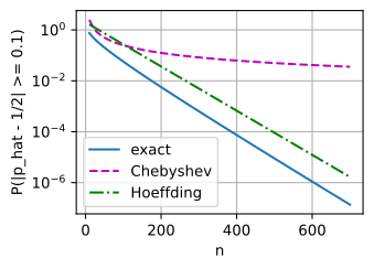
     n      exact  Chebyshev  Hoeffding
    10   7.54e-01   2.50e+00   1.64e+00
   100   5.69e-02   2.50e-01   2.71e-01
  1000   2.73e-10   2.50e-02   4.12e-09
  5000   1.30e-45   5.00e-03   7.44e-44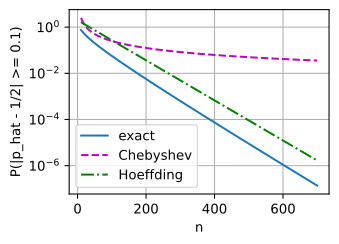
     n      exact  Chebyshev  Hoeffding
    10   7.54e-01   2.50e+00   1.64e+00
   100   5.69e-02   2.50e-01   2.71e-01
  1000   2.73e-10   2.50e-02   4.12e-09
  5000   1.30e-45   5.00e-03   7.44e-44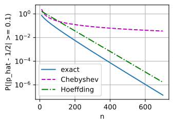
     n      exact  Chebyshev  Hoeffding
    10   7.54e-01   2.50e+00   1.64e+00
   100   5.69e-02   2.50e-01   2.71e-01
  1000   2.73e-10   2.50e-02   4.12e-09
  5000   1.30e-45   5.00e-03   7.44e-44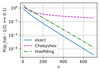
At \(n=10\) both bounds are vacuous (above \(1\)) while the exact tail is \(0.75\): nothing concentrates in ten flips. At \(n=100\) Chebyshev (\(0.25\)) is actually a shade tighter than Hoeffding (\(0.27\)): for small \(n\) the comparison is between constants, and Chebyshev’s use of the true variance \(\tfrac14\) helps it. But rates always beat constants. By \(n=1{,}000\) the exact tail is \(2.7\times10^{-10}\) and Hoeffding certifies \(4.1\times10^{-9}\), within a factor of about \(15\) (one order of magnitude), while Chebyshev still allows a miss probability of \(2.5\%\), off by eight orders of magnitude; at \(n=5{,}000\) the gap has grown to about forty-three orders. The log-scale plot makes the geometry plain: the exact tail and Hoeffding’s bound are parallel straight lines (exponential decay; Hoeffding’s exponent \(2t^2=0.02\) is close to the optimal rate, which large-deviations theory identifies as the Kullback–Leibler divergence \(\mathrm{KL}(0.6\,\|\,0.5)\approx 0.0201\), an information-theoretic measure of how distinguishable two distributions are; Section 28.2 develops both), while Chebyshev’s gentle curve is polynomial decay that no constant can rescue.
27.6.2 Probability in High Dimension
Concentration also governs the geometry of random vectors. Their coordinates provide many independent contributions, so inequalities for sums yield high-dimensional geometric results. This phenomenon is called concentration of measure: in high dimension, a sufficiently regular function of many independent coordinates is close to its expected value with high probability. This section quantifies two important examples. Section 27.2 stated two facts while cataloguing the multivariate Gaussian: the norm of a \(d\)-dimensional standard Gaussian locks onto \(\sqrt d\), and two independent draws are nearly orthogonal. Here we give both facts their quantitative treatment.
27.6.2.1 Norm Concentration
Proposition (norm concentration). Let \(\mathbf x\sim\mathcal N(\mathbf 0,\mathbf I_d)\). For every \(0<\varepsilon\le 1\),
\[ P\!\left(\Bigl|\frac{\|\mathbf x\|}{\sqrt d} - 1\Bigr| \ge \varepsilon\right) \le 2\exp\!\left(-\frac{d\,\varepsilon^2}{8}\right). \tag{27.6.7}\]
Proof sketch. The squared norm \(\|\mathbf x\|^2=\sum_{i=1}^d x_i^2\) is a sum of \(d\) i.i.d. variables \(x_i^2\) with mean \(1\): exactly a sample-mean problem, except the summands are unbounded, so Hoeffding does not apply directly. They are, however, sub-exponential, precisely the small-\(\lambda\) regime defined above. Its MGF is explicit, \(E[e^{\lambda(x_i^2-1)}] = e^{-\lambda}/\sqrt{1-2\lambda}\) for \(\lambda<\tfrac12\). A series comparison (see (Vershynin 2018), §2.7) shows
\[ E\bigl[e^{\lambda (x_i^2 - 1)}\bigr] \le e^{2\lambda^2} \qquad\textrm{for } |\lambda| \le \tfrac14 . \]
This is sub-exponentiality with \(\nu^2=4\) and \(\alpha=4\). Chernoff with this bound gives, for any \(0<\lambda\le\tfrac14\),
\[ P\Bigl(\sum_i (x_i^2 - 1) \ge d\varepsilon\Bigr) \le \exp\bigl(-\lambda d \varepsilon + 2 d \lambda^2\bigr), \]
and the unconstrained minimizer \(\lambda=\varepsilon/4\) is admissible precisely when \(\varepsilon\le 1\), yielding \(e^{-d\varepsilon^2/8}\); the lower tail and the factor \(2\) follow as in Hoeffding’s inequality. Finally convert squares to norms: writing \(z=\|\mathbf x\|/\sqrt d\ge 0\), if \(|z-1|\ge\varepsilon\) then \(|z^2-1|=|z-1|\,(z+1)\ge\varepsilon\), so the norm event implies the squared-norm event and inherits its bound.
The bound has two consequences. First, the fluctuation of \(\|\mathbf x\|\) is of constant order: deviations of \(\|\mathbf x\|\) from \(\sqrt d\) beyond \(\varepsilon\sqrt d\) are exponentially rare in \(d\), and a finer analysis puts the standard deviation of \(\|\mathbf x\|\) near \(1/\sqrt2\) independently of \(d\). A standard Gaussian in \(\mathbb{R}^d\) is therefore a thin shell of radius \(\sqrt d\) and thickness \(O(1)\), rather than a ball concentrated near the origin. Second, the point of highest density is not a typical point: the density is largest at the origin, yet the volume of a radius-\(r\) shell grows like \(r^{d-1}\), and the product of density and shell volume is largest near \(r\approx\sqrt d\). In \(d=784\) (an MNIST-sized Gaussian) a typical draw has norm within a few percent of \(28\). By Equation 27.6.7, a draw with norm below \(14\) has probability at most \(2e^{-24}\).
27.6.2.2 Near-Orthogonality Revisited
The second fact is the cosine. Section 24.1 proved that the cosine between independent random directions has mean \(0\) and standard deviation \(\approx 1/\sqrt d\); Section 27.2 restated it for Gaussians. Concentration puts that “typical” statement into the same exponential frame as everything else in this section, and the mechanism is Hoeffding again. Fix a unit vector \(\mathbf u\) and let the coordinates of \(\mathbf x\) be independent, centered, and of unit variance, either uniform random signs \(x_i\in\{-1,+1\}\) or standard Gaussians (the former are bounded, the latter sub-Gaussian with proxy \(1\) via Equation 27.6.5; either property suffices below). The inner product \(\langle\mathbf x,\mathbf u\rangle=\sum_i u_i x_i\) is a sum of independent terms, the \(i\)-th bounded by \(|u_i|\), and the general Hoeffding inequality for non-identical ranges (exercise 2) gives
\[ P\bigl(|\langle\mathbf x,\mathbf u\rangle| \ge s\bigr) \le 2\exp\!\left(-\frac{s^2}{2\sum_i u_i^2}\right) = 2 e^{-s^2/2}, \]
since \(\sum_i u_i^2=1\). The inner product with any fixed direction is \(O(1)\), while the unit-variance coordinates pin the norm of \(\mathbf x\) to \(\approx\sqrt d\): exactly \(\sqrt d\) for random signs, and within \((1\pm\varepsilon)\sqrt d\) for Gaussians by Equation 27.6.7. The cosine is therefore \(O(1/\sqrt d)\) with exponentially high probability: taking \(s=\varepsilon\sqrt d\), a cosine larger than \(\approx\varepsilon\) has probability at most \(\approx 2e^{-d\varepsilon^2/2}\). High-dimensional space holds exponentially many pairwise-nearly-orthogonal directions: a union bound over the fewer than \(m^2\) pairs among \(m\) independent draws keeps every pairwise cosine below \(\approx\varepsilon\) whenever \(2m^2 e^{-d\varepsilon^2/2}<1\), which allows \(m\) of order \(e^{d\varepsilon^2/4}\), so random directions come nearly orthogonal by default, exponentially many at a time.
27.6.2.3 Three Consequences for Deep Learning
Initialization scales. LeCun and He initialization (He et al. 2015) draw the weight rows of a layer with variance \(1/d\) (or \(2/d\) for ReLU), and the standard telling (Section 4.4) checks variances: each pre-activation \(\langle\mathbf w,\mathbf x\rangle\) has variance \(\|\mathbf x\|^2/d\approx 1\). For a single wide random layer, analogous concentration results can make this variance calculation representative: under independence or weak-dependence and tail assumptions, the empirical activation norm is close to its expectation with high probability. Iterating the statement through a deep nonlinear network is a different problem. Dependencies accumulate across layers, and preserving mean variance does not guarantee controlled singular values or dynamical isometry. A forward-pass norm check is therefore a useful diagnostic, not a proof that all signals remain stable through depth.
Distance concentration and nearest neighbors. For two independent draws the difference \(\mathbf x-\mathbf y\) is again a Gaussian vector, now with coordinate variance \(2\), so Equation 27.6.7 applies to it verbatim: each pairwise distance lands in \((1\pm\varepsilon)\sqrt{2d}\) except with probability \(2e^{-d\varepsilon^2/8}\). Among \(n\) unstructured points there are fewer than \(n^2\) pairs, and a union bound puts every distance in that shell as soon as
\[ n^2 \cdot 2e^{-d\varepsilon^2/8} \le \delta, \qquad\textrm{i.e.}\qquad d \ \ge\ \frac{8}{\varepsilon^2}\log\frac{2n^2}{\delta} : \]
a dimension only logarithmic in the number of points suffices to flatten the entire distance matrix into a band of relative width \(\varepsilon\). (File the move away for the next section: a union bound converting one exponential tail into a simultaneous guarantee over many objects, with only a logarithmic increase in the deviation, is precisely how learning bounds are built.) The nearest and farthest neighbor of a query then differ by a vanishing relative margin (the contrast \((d_{\max}-d_{\min})/d_{\min}\) collapses) and nearest-neighbor retrieval degenerates into noise-ranking. Real embeddings escape because they are structured: semantic similarity places data near a low-dimensional set inside \(\mathbb{R}^d\), so observed distance histograms are far broader than the concentration prediction, and the size of that gap is one gauge of how much structure an embedding carries.
The thin shell and the mean. The shell picture corrects a beginner’s mental model that matters in generative modeling: the “most likely point” of a high-dimensional Gaussian prior (the origin) is nowhere near a typical point. Decoders are trained on inputs of norm \(\approx\sqrt d\), so evaluating one at the mean, or at the midpoint of two latent draws (norm \(\approx\sqrt{d/2}\), well inside the shell), feeds it an input unlike anything it saw in training; this is why latent-space interpolation is done along the sphere rather than the chord. The shell is also why the MVN cell of Section 27.2 saw norm ratios pinned to \(1.000\): it was measuring means; the cell below measures the whole distribution.
27.6.2.4 Measuring the Shell
The distributions chapter verified the means of the norm ratio and cosine. We now estimate the fraction of the distribution inside the shell \((1\pm\varepsilon)\sqrt d\) and measure the reduction in nearest-neighbor contrast, using \(\varepsilon=0.1\).
rng = onp.random.default_rng(0)
eps, num_pts = 0.1, 10000
for d in (2, 20, 200, 2000):
    x = rng.standard_normal((num_pts, d))
    ratio = onp.linalg.norm(x, axis=1) / onp.sqrt(d)
    shell = onp.mean(onp.abs(ratio - 1) <= eps)      # mass in the 10% shell
    query, points = x[0], x[1:201]                   # 1 query, 200 neighbors
    dist = onp.linalg.norm(points - query, axis=1)
    contrast = (dist.max() - dist.min()) / dist.min()
    print(f'd={d:5d}:  mass within (1±0.1)·sqrt(d): {shell:6.1%},   '
          f'NN contrast (d_max-d_min)/d_min = {contrast:6.3f}')
d= 2: mass within (1±0.1)·sqrt(d): 14.8%, NN contrast (d_max-d_min)/d_min = 29.440
d= 20: mass within (1±0.1)·sqrt(d): 47.6%, NN contrast (d_max-d_min)/d_min = 1.234
d= 200: mass within (1±0.1)·sqrt(d): 95.4%, NN contrast (d_max-d_min)/d_min = 0.239
d= 2000: mass within (1±0.1)·sqrt(d): 100.0%, NN contrast (d_max-d_min)/d_min = 0.079In \(d=2\) the “shell” holds under \(15\%\) of the mass: low dimension really is a fuzzy ball, and the nearest and farthest of \(200\) points differ by a factor of \(30\). By \(d=200\) the same \(\pm10\%\) shell already captures \(95\%\) of the mass, close to what Equation 27.6.7’s Gaussian-rate reading predicts (\(\pm 2\) standard deviations at \(\sigma\approx 1/\sqrt{2d}=0.05\)), and at \(d=2000\) all ten thousand sampled points lie within the shell. The nearest-neighbor contrast decreases from \(29.4\) to \(0.08\): in \(d=2000\) the farthest of two hundred random points is only \(8\%\) farther from the query than the nearest. Distances therefore discriminate poorly among these points.
27.6.3 From One Estimate to Uniform Convergence
27.6.3.1 Data-Dependent Function Selection
We now apply the result to learning. Hoeffding’s inequality certifies the empirical risk of one fixed function: choose \(f\), then draw the sample \(S=\{(\mathbf x_i,y_i)\}_{i=1}^n\), and the empirical risk \(\hat R(f)=\frac1n\sum_i \ell(f(\mathbf x_i),y_i)\) is within \(t\) of the true risk \(R(f)=E[\ell(f(\mathbf x),y)]\) except with probability \(2e^{-2nt^2}\). A test set works exactly because it respects this order: the model was frozen before the test data were drawn. But a learner violates the order by construction: it searches a class \(\mathcal F\) and returns the \(\hat f\) that makes \(\hat R\) small on the sample it saw. The empirical risk of \(\hat f\) is a minimum of fluctuating quantities, selected precisely where the fluctuation is most favorable, and its optimism is not covered by any single-function bound. The quantity that must concentrate is the worst case over the class,
\[ \sup_{f\in\mathcal F}\ \bigl|\hat R(f) - R(f)\bigr|, \]
because if this supremum is at most \(t\) then every function’s empirical risk is trustworthy to \(t\), including whichever one the learner happens to pick. Bounds on this supremum are called uniform convergence bounds, and they are the classical mechanics that Section 4.5 waves at. The test-set reuse discussed in Section 3.6 is the same trap: an analyst who evaluates many models on one test set and reports the best is a learner whose “class” is the set of models tried. The bound we prove next quantifies this when the pool of models is fixed before the test data are drawn; what happens when it is not, we take up right after the proof.
27.6.3.2 Finite Classes: the Union Bound
For a finite class, the union bound supplies a simultaneous guarantee.
Proposition (finite-class uniform convergence). Let \(\mathcal F\) be finite, let the loss take values in \([0,1]\), and let \(S\) be an i.i.d. sample of size \(n\). Then with probability at least \(1-\delta\),
\[ \bigl|\hat R(f) - R(f)\bigr| \le \sqrt{\frac{\log(2|\mathcal F|/\delta)}{2n}} \qquad\textrm{simultaneously for every } f\in\mathcal F . \tag{27.6.8}\]
Proof. For each fixed \(f\), \(\hat R(f)\) is an average of \(n\) i.i.d. terms in \([0,1]\), so Hoeffding Equation 27.6.3 gives \(P(|\hat R(f)-R(f)|\ge t)\le 2e^{-2nt^2}\). The probability that any of the \(|\mathcal F|\) bad events occurs is at most the sum of their probabilities (the union bound again), i.e. \(2|\mathcal F|e^{-2nt^2}\). Setting this to \(\delta\) and solving for \(t\) gives the claim. \(\blacksquare\)
The effect of selecting from a class appears as \(\log|\mathcal F|\). Guaranteeing one function puts \(\log(2/\delta)\) in the numerator; allowing a choice among \(|\mathcal F|\) adds \(\log|\mathcal F|\): one extra bit of sample information per bit of selection freedom. Since the deviation shrinks like the square root, the sample size needed grows only logarithmically in the class size, which is why choosing among even thousands of hyperparameter configurations on a \(10{,}000\)-point validation set is tolerable: \(t\) grows only from \(\sqrt{\log(2/\delta)/2n}\approx 0.014\) to \(\sqrt{\log(2\cdot 2000/\delta)/2n}\approx 0.024\) at \(\delta=0.05\). Even a million models widen the guarantee only to \(\approx 0.030\), a factor of \(2.18\) over the single-function interval. But mind the hypothesis doing the work: the union bound treats \(\mathcal F\) as fixed before the sample is drawn, so this arithmetic covers a pre-registered pool of candidates. A leaderboard is different. When each submission is chosen after seeing earlier scores on the same test set, the models are data-dependent functions, the proposition’s “for each fixed \(f\)” fails, and Equation 27.6.8 does not apply; guarantees then degrade much faster, and analyzing how is the subject of adaptive data analysis (Dwork et al. 2015). This is Section 3.6’s test-set-reuse warning, now with both its constant and its boundary.
27.6.3.3 Rademacher Complexity
Real hypothesis classes are infinite (every \(\mathbf w\in\mathbb{R}^d\) is a different linear classifier), so the union bound stalls. The classical escapes either discretize the class (covering numbers: replace \(\mathcal F\) by the finitely many centers of small balls that cover it, and union-bound over those) or count its effective behaviors on \(n\) points (the VC dimension of (Vapnik and Chervonenkis 1971), sketched in Section 3.6). The modern tool is more direct, and it starts from a question a machine learner can act on: how well can the class correlate with pure noise? Let \(\varepsilon_1,\ldots,\varepsilon_n\) be i.i.d. Rademacher variables (fair random signs) and define the empirical Rademacher complexity of a class \(\mathcal F\) on the sample \(S=(\mathbf x_1,\ldots,\mathbf x_n)\) as
\[ \widehat{\mathfrak R}_S(\mathcal F) = E_{\boldsymbol\varepsilon}\!\left[\, \sup_{f\in\mathcal F}\ \frac1n \sum_{i=1}^n \varepsilon_i\, f(\mathbf x_i) \right], \tag{27.6.9}\]
with \(\mathfrak R_n(\mathcal F)=E_S[\widehat{\mathfrak R}_S(\mathcal F)]\) its average over samples. The random signs are fictitious labels containing no signal. The supremum measures how strongly functions in the class can correlate with them. If \(\widehat{\mathfrak R}\) is near \(1\), the class can fit arbitrary labels, and its empirical risks need not estimate population risks well. If \(\widehat{\mathfrak R}\) tends to zero, empirical and population risks converge uniformly. The following theorem makes this relation precise:
Uniform convergence via Rademacher complexity (Bartlett and Mendelson 2002). For \(\mathcal F\) taking values in \([0,1]\), with probability at least \(1-\delta\) over the sample,
\[ R(f) \le \hat R(f) + 2\,\mathfrak R_n(\mathcal F) + \sqrt{\frac{\log(1/\delta)}{2n}} \qquad\textrm{simultaneously for every } f\in\mathcal F . \tag{27.6.10}\]
In this statement \(\mathcal F\) is the loss class: its members are functions \((\mathbf x,y)\mapsto\ell(f(\mathbf x),y)\) taking values in \([0,1]\). We relate this class to the predictor class at the end of the subsection. We do not give the full proof, but its central move, symmetrization (the step that conjures coin flips out of a statement that contains none), is short enough to sketch, and it explains the factor \(2\). Introduce a ghost sample \(S'\): a second, fictitious dataset of size \(n\), independent of \(S\), that exists only inside the analysis. Since \(R(f)=E_{S'}[\hat R_{S'}(f)]\), Jensen’s inequality (Section 26.3.3) bounds the expected uniform deviation by a comparison of two concrete samples,
\[ E_S\Bigl[\sup_{f} \bigl(R(f) - \hat R_S(f)\bigr)\Bigr] \le E_{S,S'}\Bigl[\sup_{f} \frac1n \sum_{i=1}^n \bigl(\ell'_i(f) - \ell_i(f)\bigr)\Bigr], \]
with \(\ell_i,\ell'_i\) the losses on the \(i\)-th real and ghost points. Now the trick: \(S\) and \(S'\) are i.i.d., so swapping the \(i\)-th real and ghost points leaves the joint distribution unchanged, which means each difference \(\ell'_i-\ell_i\) can be multiplied by an independent random sign \(\varepsilon_i\) for free. Splitting the signed sum into its two halves leaves \(2\,E[\sup_f \frac1n\sum_i \varepsilon_i \ell_i(f)] = 2\,\mathfrak R_n(\ell\circ\mathcal F)\): the unknown truth has vanished, and a correlation with coin flips stands in its place. The final step from this statement in expectation to the high-probability form Equation 27.6.10 is McDiarmid’s inequality (McDiarmid 1989), the extension of Hoeffding from sums to any function that no single coordinate can move much (here, changing one sample point moves the supremum by at most \(1/n\)); it is stated in exercise 3, where it also puts an error bar on the bootstrap. Sanity-check the theorem at its ends. A singleton class has \(\widehat{\mathfrak R}=0\) (the expectation of \(\frac1n\sum\varepsilon_i f(\mathbf x_i)\) is \(0\) with nothing to optimize) and Equation 27.6.10 collapses to one-sided Hoeffding. A finite class obeys \(\mathfrak R_n \le \sqrt{2\log|\mathcal F|/n}\) (Massart’s lemma (Boucheron et al. 2013)), recovering Equation 27.6.8 up to constants. For binary classes, the growth function and VC dimension bound the number of labelings that the class can realize on \(n\) points, giving \(\mathfrak R_n\lesssim\sqrt{d_{\mathrm{VC}}\log n / n}\) (Boucheron et al. 2005). At the other end, the class of all functions into \([-1,1]\) matches every sign pattern perfectly, \(\widehat{\mathfrak R}=1\), and the bound is vacuous, as it must be, since that class can memorize anything.
27.6.3.4 The Linear Class in Closed Form
Rademacher complexity is useful when it can be bounded or computed. For norm-constrained linear functions, the calculation is short and leads directly to a dimension-independent bound.
Proposition (Rademacher complexity of a norm-bounded linear class). Let \(\mathcal F=\{\mathbf x\mapsto\langle\mathbf w,\mathbf x\rangle : \|\mathbf w\|_2\le B\}\) and suppose the sample satisfies \(\|\mathbf x_i\|_2\le r\) for all \(i\). Then
\[ \widehat{\mathfrak R}_S(\mathcal F) \le \frac{B\,r}{\sqrt n}. \tag{27.6.11}\]
Proof. The supremum is explicit: by linearity and Cauchy–Schwarz (with equality at \(\mathbf w\) aligned to the sum),
\[ \sup_{\|\mathbf w\|\le B}\ \frac1n\sum_{i=1}^n \varepsilon_i \langle\mathbf w,\mathbf x_i\rangle = \sup_{\|\mathbf w\|\le B}\ \frac1n \Bigl\langle\mathbf w,\ \sum_i \varepsilon_i\mathbf x_i\Bigr\rangle = \frac Bn\,\Bigl\|\sum_{i=1}^n \varepsilon_i\mathbf x_i\Bigr\| . \]
Jensen’s inequality (Section 26.3.3; the square root is concave) moves the expectation inside the square:
\[ E_{\boldsymbol\varepsilon}\Bigl\|\sum_i\varepsilon_i\mathbf x_i\Bigr\| \le \sqrt{E_{\boldsymbol\varepsilon}\Bigl\|\sum_i\varepsilon_i\mathbf x_i\Bigr\|^2} = \sqrt{\sum_{i,j} E[\varepsilon_i\varepsilon_j]\, \langle\mathbf x_i,\mathbf x_j\rangle} = \sqrt{\sum_i \|\mathbf x_i\|^2} \le r\sqrt n, \]
the cross terms vanishing because independent signs have \(E[\varepsilon_i\varepsilon_j]=0\) for \(i\ne j\). Multiplying by \(B/n\) gives \(Br/\sqrt n\). \(\blacksquare\)
Now look at what is absent from Equation 27.6.11: the dimension \(d\). A linear class over a million features and over ten features has the same bound only when both its weight-radius \(B\) and input-radius \(r\) match. Thus parameter count does not appear explicitly; capacity in this bound is controlled by the product \(Br\). Changing or adding features can change \(r\), so weight norm alone is not an invariant measure of capacity. The bound nevertheless gives one reason norm control can help: shrinking \(\|\mathbf w\|\) permits a smaller radius \(B\) when the class is specified independently of the sample. This connects to weight decay (Section 2.7) and motivates tracking solution norm below. It does not by itself explain the double-descent experiment, because feature radii and data-dependent selection also matter.
One step connects the two propositions. Equation 27.6.10 wants the complexity of the loss class \(\ell\circ\mathcal F\) (the functions whose empirical means we actually compare), while Equation 27.6.11 computes that of the predictor class \(\mathcal F\). The bridge is the contraction principle (Boucheron et al. 2013): composing every \(f\in\mathcal F\) with one fixed \(L\)-Lipschitz function \(\phi\) multiplies the Rademacher complexity by at most \(L\) after centering \(\phi(0)=0\); subtracting the constant \(\phi(0)\) does not affect the signed complexity. Thus \(\widehat{\mathfrak R}_S(\phi\circ\mathcal F)\le L\,\widehat{\mathfrak R}_S(\mathcal F)\). Margin losses (the hinge, the clipped square, the logistic) are Lipschitz in the prediction, so the loss class of the norm-bounded linear model inherits the bound \(L\,Br/\sqrt n\) and the norm-controls-capacity conclusion survives the composition intact.
27.6.3.5 Vacuous Bounds and Useful Complexity Measures
For modern neural networks, these bounds are often vacuous. (Zhang et al. 2021) trained standard architectures to zero training error on CIFAR-10 with randomly shuffled labels (on ImageNet, random-label training still reaches near-perfect training accuracy): the class realized by “this architecture, trained by SGD” can correlate essentially perfectly with coin flips, so its Rademacher complexity on such samples is essentially \(1\) and Equation 27.6.10 certifies nothing; norm-based refinements, evaluated at the sizes practitioners use, yield bounds orders of magnitude above the trivial bound of \(1\). This is a fact about these bounds, the ones that take uniform convergence over the entire representable class. The same architecture can generalize on real labels, showing that the data, optimizer, and reached solution contain information ignored by a bound on the entire representable class. Subsequent work therefore studies smaller, algorithm- or data-dependent classes. Uniform convergence provides one precise form of a generalization guarantee, but it is not the only framework for analyzing learning algorithms. Here the crude choice of \(\mathcal F\) makes the displayed bound vacuous. The last section studies a smaller random-features model in which solution norm and conditioning can be computed directly.
27.6.3.6 Coin Flips in Code
Both phenomena can be measured. First we estimate \(\widehat{\mathfrak R}_S\) for the norm-bounded linear class by Monte Carlo: the proof gave the supremum in closed form, \(\frac Bn\|\sum_i\varepsilon_i\mathbf x_i\|\), so we average that norm over random sign draws and compare against \(Br/\sqrt n\). Then we exhibit the Zhang phenomenon in miniature: a class rich enough to interpolate (here, minimum-norm least squares on \(p=2n\) random features, via the pseudoinverse of Section 24.3.3.1) achieves correlation \(1\) with every coin flip it is shown.
rng = onp.random.default_rng(0)
n, d, B, num_sigma = 50, 20, 1.0, 2000
X = rng.standard_normal((n, d))
X /= onp.linalg.norm(X, axis=1, keepdims=True)     # ||x_i|| = r = 1
signs = rng.choice([-1.0, 1.0], size=(num_sigma, n))
sup_corr = B * onp.linalg.norm(signs @ X, axis=1) / n  # closed-form supremum
print(f'Monte-Carlo Rademacher complexity  = {sup_corr.mean():.4f}')
print(f'bound B*r/sqrt(n)                  = {B / onp.sqrt(n):.4f}')

# The Zhang phenomenon in miniature: an interpolating class hits corr = 1
Phi = rng.standard_normal((n, 2 * n))        # p = 2n features: interpolation
W = onp.linalg.pinv(Phi) @ signs.T           # min-norm fit to every flip set
corr = onp.mean(signs.T * (Phi @ W), axis=0)     # (1/n) sum_i eps_i f(x_i)
w_norm = onp.linalg.norm(W, axis=0).mean()
r_phi = onp.linalg.norm(Phi, axis=1).mean()
print(f'correlation of min-norm fits with coin flips = {corr.mean():.4f}')
print(f'norm it costs: mean ||w|| = {w_norm:.2f};  implied capacity bound '
      f'B*r/sqrt(n) = {w_norm * r_phi / onp.sqrt(n):.2f}')
Monte-Carlo Rademacher complexity = 0.1390
bound B*r/sqrt(n) = 0.1414
correlation of min-norm fits with coin flips = 1.0000
norm it costs: mean ||w|| = 1.00; implied capacity bound B*r/sqrt(n) = 1.41The Monte-Carlo estimate is \(0.1390\) against the bound \(0.1414\): the Cauchy–Schwarz/Jensen argument is nearly tight, losing under \(2\%\) (the only slack is Jensen’s step, and \(\|\sum\varepsilon_i\mathbf x_i\|\) has small relative fluctuation: concentration again). So a unit-norm linear class on fifty unit-norm points can fake a correlation of about \(0.14\) with pure noise, and no more: its empirical risks are meaningful. The interpolating class, by contrast, scores a correlation of exactly \(1.0000\) on every one of the two thousand sign patterns; it is the all-functions endpoint of the theorem, in twenty features and fifty points. The norm it needed is printed next to it: the sign-fitting solutions need norm about \(1.0\) on features of norm about \(10\), so the smallest linear class containing them has capacity bound \(Br/\sqrt n\approx 1.41 > 1\), vacuous, exactly as the previous subsection said it must be. The two prints summarize the section: the capacity that matters is the norm the fit actually uses on the data.
27.6.4 Interpolation and Double Descent
27.6.4.1 Classical U-Shaped Risk Curves
The familiar U-curve is a useful heuristic: as a model class grows, bias may fall while variance rises. Neither the bias–variance identity nor uniform convergence requires this shape, however. In some interpolating regimes, test error peaks near the point where training error first reaches zero and then falls as the model grows. This behavior is called double descent (Belkin et al. 2019; Nakkiran et al. 2021). Section 4.5 surveys empirical examples in deep learning. Here we analyze one controlled random-features regression experiment. Its conditioning and minimum-norm mechanisms are exact for this construction; they should not be read as a general explanation of deep-network generalization.
27.6.4.2 The Minimum-Norm Mechanism
The smallest such model is random-features regression (Rahimi and Recht 2007). Fix a feature map built from randomness (ours will be \(\phi(\mathbf x)=\mathrm{ReLU} (\mathbf V\mathbf x)\) with a random frozen \(\mathbf V\), a one-hidden-layer network whose first layer is never trained) and fit only the linear head \(\mathbf w\in\mathbb{R}^p\) by least squares on \(n\) training points. The We vary the feature count \(p\) across the interpolation threshold \(p=n\). The fitted model behaves differently below, at, and above this threshold. Write \(\boldsymbol\Phi\in\mathbb{R}^{n\times p}\) for the feature matrix and fit \(\mathbf w=\boldsymbol\Phi^{+}\mathbf y\) with the pseudoinverse of Section 24.3.3.1, which returns the least-squares solution for \(p<n\) and the minimum-norm interpolant for \(p\ge n\).
Below the threshold (\(p<n\)) the system is overdetermined: the fit cannot match all \(n\) labels, residual noise is averaged rather than reproduced, and the classical U-curve logic applies verbatim: bias falls and variance rises with \(p\).
At the threshold (\(p=n\)) the feature matrix is square, and interpolation requires inverting it: \(\mathbf w=\boldsymbol\Phi^{-1}\mathbf y\). A random square matrix is almost surely invertible but almost never well invertible: its smallest singular value \(\sigma_{\min}\) is typically tiny, and the condition-number lens of Section 24.3.3.2 says what happens next: the solution acquires a component of size \(\langle\mathbf u_{\min},\mathbf y\rangle/\sigma_{\min}\) along the worst direction. The labels’ noise, which a regression is supposed to average away, is instead divided by a near-zero number. The solution norm explodes and the test error spikes. This is the peak of double descent, and it is a conditioning event.
Beyond the threshold (\(p>n\)) interpolation is easy: infinitely many \(\mathbf w\) fit exactly, and the pseudoinverse picks the smallest. With nested features (each model uses the first \(p\) columns of one master matrix) this yields an exact monotonicity: any interpolant available at \(p\) is still available at \(p+1\) by padding with a zero, so the feasible set only grows and
\[ \bigl\|\mathbf w^{(p+1)}_{\min}\bigr\| \le \bigl\|\mathbf w^{(p)}_{\min}\bigr\| : \]
more nested features let the minimum-norm interpolant get no larger. This is a useful part of the mechanism, but it is not by itself a Rademacher-complexity proof of the second descent. The bound Equation 27.6.11 depends on \(Br\): as \(p\) grows here, \(\|\mathbf w\|\) falls while the random-feature norm \(\|\boldsymbol\phi(\mathbf x)\|\) grows. Moreover, selecting the radius from the fitted, data-dependent solution requires a localized or algorithm-dependent argument. The experiment below therefore tracks solution norm as a diagnostic correlated with test error, not as a complete capacity certificate.
27.6.4.3 A Numerical Double-Descent Example
We now compute the complete double-descent curve. We use forty training points from a noisy linear teacher in fifteen dimensions; ReLU random features with nested columns; the head fit by pinv: least squares below the threshold, minimum-norm interpolation above it. We sweep \(p\) from \(2\) to \(400\) straight through \(p=n=40\), and we track the two quantities the mechanism says to watch: the test error and \(\|\mathbf w\|\). Medians over \(20\) independent runs keep the curve readable.
rng = onp.random.default_rng(0)
n, n_test, d_in, p_max, trials, noise = 40, 500, 15, 400, 20, 0.1
p_grid = onp.array([2, 5, 10, 15, 20, 25, 30, 35, 38, 40, 42, 45, 50, 60,
                    80, 120, 200, 400])
test_mse, train_mse, w_norm = (onp.zeros((trials, len(p_grid)))
                               for _ in range(3))
for tr in range(trials):
    beta = rng.standard_normal(d_in)
    beta /= onp.linalg.norm(beta)                    # teacher: y = <beta, x>
    X, X_te = (rng.standard_normal((m, d_in)) for m in (n, n_test))
    y = X @ beta + noise * rng.standard_normal(n)    # noisy training labels
    y_te = X_te @ beta
    V = rng.standard_normal((p_max, d_in)) / onp.sqrt(d_in)
    Phi, Phi_te = onp.maximum(X @ V.T, 0), onp.maximum(X_te @ V.T, 0)
    for j, p in enumerate(p_grid):                   # nested feature prefixes
        w = onp.linalg.pinv(Phi[:, :p]) @ y  # least-squares/min-norm solution
        test_mse[tr, j] = onp.mean((Phi_te[:, :p] @ w - y_te) ** 2)
        train_mse[tr, j] = onp.mean((Phi[:, :p] @ w - y) ** 2)
        w_norm[tr, j] = onp.linalg.norm(w)
med = [onp.median(a, axis=0) for a in (test_mse, train_mse, w_norm)]
for j, p in enumerate(p_grid):
    print(f'p={p:3d}  test MSE={med[0][j]:9.4f}  train MSE={med[1][j]:9.2e}'
          f'  ||w||={med[2][j]:7.2f}')
d2l.plot(p_grid, [med[0], med[2]], 'number of random features p',
         'median over 20 runs', legend=['test MSE', '||w|| of the fit'],
xscale='log', yscale='log')p= 2 test MSE= 1.0378 train MSE= 8.67e-01 ||w||= 0.32
p= 5 test MSE= 0.9627 train MSE= 7.70e-01 ||w||= 0.77
p= 10 test MSE= 0.7728 train MSE= 4.64e-01 ||w||= 1.68
p= 15 test MSE= 0.6782 train MSE= 2.81e-01 ||w||= 1.97
p= 20 test MSE= 0.7156 train MSE= 1.54e-01 ||w||= 2.15
p= 25 test MSE= 0.6905 train MSE= 8.10e-02 ||w||= 2.37
p= 30 test MSE= 0.6893 train MSE= 4.32e-02 ||w||= 2.70
p= 35 test MSE= 1.5061 train MSE= 1.32e-02 ||w||= 3.75
p= 38 test MSE= 2.1205 train MSE= 5.00e-03 ||w||= 4.61
p= 40 test MSE= 33.6376 train MSE= 1.00e-28 ||w||= 18.52
p= 42 test MSE= 1.9858 train MSE= 1.15e-29 ||w||= 4.96
p= 45 test MSE= 1.1249 train MSE= 7.16e-30 ||w||= 3.64
p= 50 test MSE= 0.6466 train MSE= 7.35e-30 ||w||= 2.42
p= 60 test MSE= 0.3507 train MSE= 5.36e-30 ||w||= 1.70
p= 80 test MSE= 0.1824 train MSE= 5.72e-30 ||w||= 1.18
p=120 test MSE= 0.1121 train MSE= 7.99e-30 ||w||= 0.83
p=200 test MSE= 0.0796 train MSE= 9.07e-30 ||w||= 0.59
p=400 test MSE= 0.0604 train MSE= 7.00e-30 ||w||= 0.39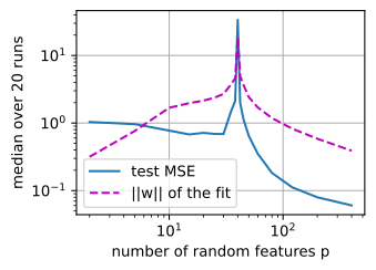
p=  2  test MSE=   1.0378  train MSE= 8.67e-01  ||w||=   0.32
p=  5  test MSE=   0.9627  train MSE= 7.70e-01  ||w||=   0.77
p= 10  test MSE=   0.7728  train MSE= 4.64e-01  ||w||=   1.68
p= 15  test MSE=   0.6782  train MSE= 2.81e-01  ||w||=   1.97
p= 20  test MSE=   0.7156  train MSE= 1.54e-01  ||w||=   2.15
p= 25  test MSE=   0.6905  train MSE= 8.10e-02  ||w||=   2.37
p= 30  test MSE=   0.6893  train MSE= 4.32e-02  ||w||=   2.70
p= 35  test MSE=   1.5061  train MSE= 1.32e-02  ||w||=   3.75
p= 38  test MSE=   2.1205  train MSE= 5.00e-03  ||w||=   4.61
p= 40  test MSE=  33.6376  train MSE= 1.00e-28  ||w||=  18.52
p= 42  test MSE=   1.9858  train MSE= 1.15e-29  ||w||=   4.96
p= 45  test MSE=   1.1249  train MSE= 7.16e-30  ||w||=   3.64
p= 50  test MSE=   0.6466  train MSE= 7.35e-30  ||w||=   2.42
p= 60  test MSE=   0.3507  train MSE= 5.36e-30  ||w||=   1.70
p= 80  test MSE=   0.1824  train MSE= 5.72e-30  ||w||=   1.18
p=120  test MSE=   0.1121  train MSE= 7.99e-30  ||w||=   0.83
p=200  test MSE=   0.0796  train MSE= 9.07e-30  ||w||=   0.59
p=400  test MSE=   0.0604  train MSE= 7.00e-30  ||w||=   0.39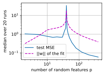
p=  2  test MSE=   1.0378  train MSE= 8.67e-01  ||w||=   0.32
p=  5  test MSE=   0.9627  train MSE= 7.70e-01  ||w||=   0.77
p= 10  test MSE=   0.7728  train MSE= 4.64e-01  ||w||=   1.68
p= 15  test MSE=   0.6782  train MSE= 2.81e-01  ||w||=   1.97
p= 20  test MSE=   0.7156  train MSE= 1.54e-01  ||w||=   2.15
p= 25  test MSE=   0.6905  train MSE= 8.10e-02  ||w||=   2.37
p= 30  test MSE=   0.6893  train MSE= 4.32e-02  ||w||=   2.70
p= 35  test MSE=   1.5061  train MSE= 1.32e-02  ||w||=   3.75
p= 38  test MSE=   2.1205  train MSE= 5.00e-03  ||w||=   4.61
p= 40  test MSE=  33.6376  train MSE= 1.00e-28  ||w||=  18.52
p= 42  test MSE=   1.9858  train MSE= 1.15e-29  ||w||=   4.96
p= 45  test MSE=   1.1249  train MSE= 7.16e-30  ||w||=   3.64
p= 50  test MSE=   0.6466  train MSE= 7.35e-30  ||w||=   2.42
p= 60  test MSE=   0.3507  train MSE= 5.36e-30  ||w||=   1.70
p= 80  test MSE=   0.1824  train MSE= 5.72e-30  ||w||=   1.18
p=120  test MSE=   0.1121  train MSE= 7.99e-30  ||w||=   0.83
p=200  test MSE=   0.0796  train MSE= 9.07e-30  ||w||=   0.59
p=400  test MSE=   0.0604  train MSE= 7.00e-30  ||w||=   0.39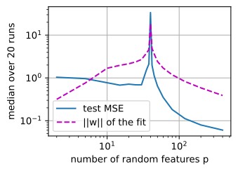
p=  2  test MSE=   1.0378  train MSE= 8.67e-01  ||w||=   0.32
p=  5  test MSE=   0.9627  train MSE= 7.70e-01  ||w||=   0.77
p= 10  test MSE=   0.7728  train MSE= 4.64e-01  ||w||=   1.68
p= 15  test MSE=   0.6782  train MSE= 2.81e-01  ||w||=   1.97
p= 20  test MSE=   0.7156  train MSE= 1.54e-01  ||w||=   2.15
p= 25  test MSE=   0.6905  train MSE= 8.10e-02  ||w||=   2.37
p= 30  test MSE=   0.6893  train MSE= 4.32e-02  ||w||=   2.70
p= 35  test MSE=   1.5061  train MSE= 1.32e-02  ||w||=   3.75
p= 38  test MSE=   2.1205  train MSE= 5.00e-03  ||w||=   4.61
p= 40  test MSE=  33.6376  train MSE= 9.58e-29  ||w||=  18.52
p= 42  test MSE=   1.9858  train MSE= 1.09e-29  ||w||=   4.96
p= 45  test MSE=   1.1249  train MSE= 7.10e-30  ||w||=   3.64
p= 50  test MSE=   0.6466  train MSE= 7.80e-30  ||w||=   2.42
p= 60  test MSE=   0.3507  train MSE= 5.29e-30  ||w||=   1.70
p= 80  test MSE=   0.1824  train MSE= 5.00e-30  ||w||=   1.18
p=120  test MSE=   0.1121  train MSE= 6.61e-30  ||w||=   0.83
p=200  test MSE=   0.0796  train MSE= 8.08e-30  ||w||=   0.59
p=400  test MSE=   0.0604  train MSE= 8.04e-30  ||w||=   0.39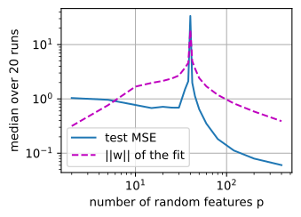
In the underparameterized regime, test error falls from \(1.04\) at \(p=2\) to about \(0.68\) around \(p=15\), then rises as variance increases. At the interpolation threshold \(p=40=n\), the training error drops from \(5\times10^{-3}\) to \(10^{-28}\) (exact interpolation, up to floating point). At the same point, the test error rises to \(33.6\), about fifty times its underparameterized minimum, while \(\|\mathbf w\|\) increases to \(18.5\). This is the effect of dividing the noise component by the small singular value \(\sigma_{\min}\). Beyond the threshold, from \(p=42\) onward, the norm decreases monotonically (\(4.96\), \(3.64\), \(2.42\), \(1.70\), \(1.18\), down to \(0.39\) at \(p=400\); the nesting guarantees this). The test error falls to \(0.65\) at \(p=50\), \(0.18\) at \(p=80\), and \(0.060\) at \(p=400\), ten times below the best underparameterized value. By contrast, the training error remains zero up to floating point everywhere past the threshold (the table prints \(10^{-28}\)), so no empirical-risk-based criterion can tell these models apart; the solution norm distinguishes them in this experiment. The Rademacher calculation motivates looking beyond parameter count, but its relevant product also includes feature norms and does not by itself predict this test curve. The best model in this entire experiment is the most overparameterized one, fitting noisy data exactly, with ten times more parameters than data points.
27.6.4.4 Benign Overfitting
One puzzle remains inside the mechanism. The \(p=400\) model interpolates its noisy labels (it reproduces every corrupted \(y_i\) exactly), yet its test error is the best on the table. When does fitting noise not hurt? The minimum-norm solution splits across the spectrum of the feature matrix: the signal is captured along the few directions with large singular values, while interpolating the residual noise is distributed (because minimizing the norm spreads it) across the many directions with small singular values, where each contaminates predictions at new points only faintly. Overfitting is benign when the spectrum has this shape: a few strong directions to carry the signal, plus a large reservoir of weak directions that absorb and average out the noise, in effect performing implicit regularization without a regularizer. (Bartlett et al. 2020) make this exact for linear regression, characterizing benignity via two effective ranks of the covariance, and (Belkin et al. 2019) frame the modern regime it explains; (Bartlett et al. 2021) survey the fast-growing theory. For deep networks the picture is instructive but not settled: features there are learned, reshaping the spectrum during training, and a theory that predicts a given network’s test error from first principles remains open.
27.6.5 Summary
- The Chernoff method (Markov’s inequality applied to \(e^{\lambda X}\), then optimized over \(\lambda\)) converts a bound on the moment generating function into an exponential tail bound; for sums of independent variables the MGF factorizes, which is where the exponential-in-\(n\) decay comes from.
- Hoeffding’s lemma bounds the MGF of a centered variable on \([a,b]\) by \(e^{\lambda^2(b-a)^2/8}\) (proof: the second derivative of the log-MGF is a tilted variance, at most \((b-a)^2/4\)), and Hoeffding’s inequality follows: \(P(|\bar X-E\bar X|\ge t)\le 2e^{-2nt^2/(b-a)^2}\), the finite-sample bound behind the main book’s test-set arithmetic, exponentially sharper than Chebyshev’s \(1/n\). Inverted, it gives the finite-sample confidence interval Equation 27.6.4. Sub-Gaussian variables are those obeying such an MGF bound; Bernstein’s inequality refines the constant using the true variance and covers the sub-exponential case (squares, norms).
- In high dimension, concentration is geometry (concentration of measure): \(\|\mathbf x\|/\sqrt d\) concentrates at \(1\) with failure probability \(2e^{-d\varepsilon^2/8}\), so a Gaussian is a thin shell, random directions are near-orthogonal (\(\cos\approx 1/\sqrt d\)), pairwise distances concentrate (degrading nearest-neighbor contrast). In a single wide random layer, related concentration can make the variance calculation representative, but stability across many nonlinear layers needs additional dependence and Jacobian control.
- Hoeffding certifies one pre-chosen function; a learner chooses after seeing data, so guarantees must hold uniformly over the class. For finite classes the union bound gives deviation \(\sqrt{\log(2|\mathcal F|/\delta)/2n}\), valid for a pool of models fixed before the data are drawn; genuinely adaptive test-set reuse voids the union bound, and its guarantees degrade faster (adaptive data analysis).
- Rademacher complexity (how well a class can correlate with random signs) bounds uniform deviations: \(R(f)\le\hat R(f)+2\mathfrak R_n(\mathcal F)+\sqrt{\log(1/\delta)/2n}\). For the linear class \(\{\|\mathbf w\|\le B\}\) on data with \(\|\mathbf x\|\le r\) it computes to \(Br/\sqrt n\): parameter count is absent when the weight and data radii are held fixed. A class rich enough to fit arbitrary random signs has complexity near its maximum and yields a vacuous bound; the failure belongs to the crude class choice, and uniform convergence survives as the language of guarantees.
- Double descent: sweeping random features through the interpolation threshold \(p=n\), test error follows the classical U, spikes at \(p=n\) (a near-singular system divides noise by \(\sigma_{\min}\)), then descends again while the minimum-norm interpolant shrinks with added nested features. This norm trend is a mechanism and diagnostic; a formal capacity explanation must also track feature norms and the data-dependent selection of the solution. Interpolating noise is benign when a few strong spectral directions carry the signal and many weak ones absorb the noise.
27.6.6 Exercises
- Prove that a Rademacher variable is sub-Gaussian with variance proxy \(1\): show \(\cosh\lambda\le e^{\lambda^2/2}\) by comparing the two Taylor series term by term (\((2k)!\ge 2^k k!\)). Conclude via the Chernoff method that an average of \(n\) fair random signs satisfies \(P(|\bar\varepsilon|\ge t)\le 2e^{-nt^2/2}\).
- The proof of Equation 27.6.3 assumed a common range \([a,b]\). Redo it for independent \(X_i\in[a_i,b_i]\) to obtain \(P(|\bar X-E\bar X|\ge t)\le 2\exp\bigl(-2n^2t^2/\sum_i(b_i-a_i)^2\bigr)\), and check that it reduces to Equation 27.6.3 when the ranges agree. This weighted version is the one the near-orthogonality argument used, with weights \(u_i\).
- McDiarmid’s inequality (McDiarmid 1989) extends Hoeffding from sums to arbitrary functions with bounded differences: if changing the \(i\)-th argument of \(g(x_1,\ldots,x_n)\) moves its value by at most \(c_i\), then \(P(|g - E[g]|\ge t)\le 2\exp\bigl(-2t^2/\sum_i c_i^2\bigr)\). Take this statement on faith (its proof needs martingales). (i) Recover Hoeffding’s inequality from it. (ii) The bootstrap of Section 27.5 computes a statistic of \(n\) data points; argue that if that statistic has bounded differences \(c_i=c/n\), the bootstrap’s ideal target (the statistic’s deviation from its mean) already concentrates at rate \(e^{-2nt^2/c^2}\), and check the median of a sample does not have small bounded differences in general.
- Compute the Rademacher complexity of the \(\ell_1\)-ball class \(\mathcal F=\{\mathbf x\mapsto\langle\mathbf w,\mathbf x\rangle: \|\mathbf w\|_1\le B\}\) on data with \(\|\mathbf x_i\|_\infty\le r\). The supremum step now uses the duality between the \(\ell_1\) and \(\ell_\infty\) norms, giving \(\frac Bn E\|\sum_i\varepsilon_i\mathbf x_i\|_\infty\); bound the expected max of \(d\) sub-Gaussian coordinates to conclude \(\widehat{\mathfrak R}_S\le Br\sqrt{2\log(2d)/n}\). Why does dimension now enter, and only logarithmically?
- Rerun the double-descent sweep with ridge regression, \(\mathbf w_\lambda=(\boldsymbol\Phi^\top\boldsymbol\Phi+ \lambda\mathbf I)^{-1}\boldsymbol\Phi^\top\mathbf y\), for \(\lambda\in\{10^{-8},10^{-4},10^{-2},1\}\). Watch the interpolation peak melt as \(\lambda\) grows, and explain why using Section 26.5: the ridge term lifts \(\sigma_{\min}^2\) to \(\sigma_{\min}^2+\lambda\), capping the noise amplification. Verify numerically that as \(\lambda\to0\) the ridge solution converges to the pseudoinverse (minimum-norm) solution.
- In the double-descent experiment, vary the label noise (\(\textrm{noise}\in\{0,\ 0.1,\ 0.5,\ 1.0\}\)) and measure the height and location of the peak. Confirm that the peak stays at \(p=n\) (its location is a rank condition, independent of the labels) while its height grows with the noise variance, and explain both observations with the \(\sigma_{\min}\) mechanism. What happens to the peak when \(\textrm{noise}=0\), and why is it not entirely gone?
- Use Equation 27.6.7 to find the smallest dimension \(d\) at which the shell \((1\pm 0.01)\sqrt d\) is guaranteed to hold at least \(99\%\) of a standard Gaussian’s mass, then estimate the true smallest \(d\) by simulation. How large is the gap, and which side of the story (rate or constant) does it come from?
- An analyst fixes a pool of \(m\) models before seeing the data, evaluates all of them on one validation set of \(n\) points (losses in \([0,1]\)), and reports the best score. Apply Equation 27.6.8 with \(\mathcal F\) the pre-registered pool to bound how optimistic the reported score can be, and evaluate the bound at \(m=10\), \(10^3\), and \(10^6\) with \(n=10{,}000\) and \(\delta=0.05\). At what \(m\) does the guaranteed accuracy degrade past \(\pm 0.02\)? Compare with the Bonferroni discussion of multiple testing in Section 27.5: which bound is doing the same job, and where do the two analyses differ? Finally, explain why none of this applies verbatim when each model is chosen after seeing the previous models’ scores (Dwork et al. 2015).