from d2l import torch as d2l
import torch8.4 Recurrent Neural Networks
In Section 8.3 we introduced \(n\)-gram models, where the conditional probability of a token \(x_t\) at time step \(t\) depends only on the \(n-1\) preceding tokens. To let tokens earlier than time step \(t-(n-1)\) influence \(x_t\) we would have to increase \(n\), but the number of parameters grows exponentially with it: we must store \(|\mathcal{V}|^n\) numbers for a vocabulary \(\mathcal{V}\). Rather than model \(P(x_t \mid x_{t-1}, \ldots, x_1)\) directly, then, it is preferable to use a latent variable model,
\[P(x_t \mid x_{t-1}, \ldots, x_1) \approx P(x_t \mid h_{t-1}), \tag{8.4.1}\]
where \(h_{t-1}\) is a hidden state that stores the sequence information up to time step \(t-1\). In general, the hidden state at any time step \(t\) can be computed from both the current input \(x_{t}\) and the previous hidden state \(h_{t-1}\):
\[h_t = f(x_{t}, h_{t-1}). \tag{8.4.2}\]
The approximation becomes exact only when \(h_{t-1}\) is a sufficient statistic of the prefix for predicting \(x_t\): \(P(x_t\mid x_{<t})=P(x_t\mid h_{t-1})\). An idealized real-valued state could encode an arbitrarily long prefix with unbounded precision, but that construction is neither robust nor operationally useful. Practical finite states impose an information bottleneck, so the model must learn which parts of the past matter for prediction.
Recall the hidden layers and hidden units of Chapter 4. It is worth stressing that hidden layers and hidden states name two very different things. Hidden layers are layers that are hidden from view on the path from input to output. Hidden states are, technically speaking, inputs to whatever we compute at a given step, and they can only be computed from data seen at earlier time steps.
Recurrent neural networks (RNNs) are neural networks with hidden states. Before defining the RNN, we first revisit the MLP of Section 4.1.
from d2l import tensorflow as d2l
import tensorflow as tf
from d2l import jax as d2l
import jax
from jax import numpy as jnpfrom d2l import mxnet as d2l
from mxnet import np, npx
npx.set_np()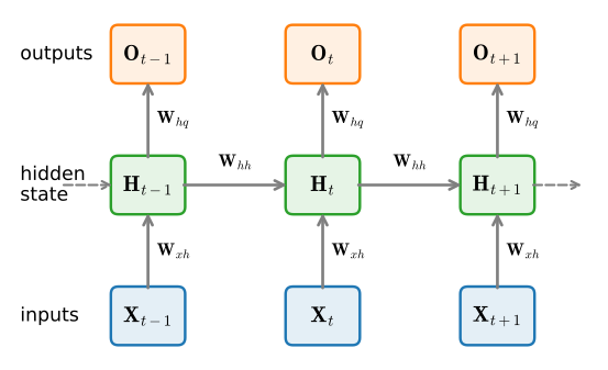
8.4.3 RNN Language Models
Recall from Section 8.3 that a language model predicts the next token from the current and past tokens, so we obtain training targets by shifting the input sequence forward by one token. Bengio et al. (2003) first used a neural network for this task; an RNN does it with a hidden state in place of a fixed window.
We tokenize text with the byte-pair encoding (BPE) tokenizer of Section 8.2, which splits text into subword tokens drawn from a fixed vocabulary \(\mathcal{V}\). (Earlier presentations of RNN language models tokenized into single characters; subword tokens give shorter sequences for the same text and are what modern language models actually use.) A token is not fed to the network as a raw id. Instead each id indexes a learned embedding table and returns a \(d\)-dimensional vector; stacking the vectors of a minibatch at step \(t\) gives the input \(\mathbf{X}_t \in \mathbb{R}^{n \times d}\). This embedding lookup replaces the one-hot encoding used in older treatments. It is the same operation, selecting one row of a matrix per token, but the rows are trained rather than fixed, and the table is looked up directly instead of materializing a one-hot vector of length \(|\mathcal{V}|\).
At each step the hidden state \(\mathbf{H}_t\) is mapped by the output layer to a vector of \(|\mathcal{V}|\) logits, one per vocabulary token, and a softmax turns these into \(P(x_{t+1} \mid x_t, \ldots, x_1)\), the model’s distribution over the next token. Because \(\mathbf{H}_t\) summarizes the entire prefix, the RNN expresses the full autoregressive factorization \(P(x_1, \ldots, x_T) = \prod_{t} P(x_t \mid x_{t-1}, \ldots, x_1)\) with no Markov truncation.
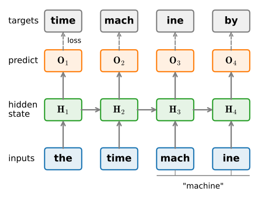
Figure 8.4.2 shows the training setup. Suppose the corpus contains “the time machine by”, which the BPE tokenizer splits into the tokens the, time, mach, ine, by (the word “machine” becomes the two subword tokens mach and ine). The input sequence is the, time, mach, ine, and the target sequence is the same stream shifted forward by one token, time, mach, ine, by. At every step we run a softmax over the output and compute the cross-entropy against the target token, then average the losses over the sequence. Because of the recurrence, the output \(\mathbf{O}_3\) is determined by the inputs the, time, mach, so its loss measures how well the model predicts the next token ine from that prefix. Minimizing perplexity is exactly this objective, since perplexity (Section 8.3) is the exponentiated average cross-entropy.
8.4.3.1 Teacher Forcing
Notice what the model consumes during training: at each step its input is the ground-truth previous token, taken from the corpus, regardless of what the model itself predicted the step before. Training a sequence model on the true prefixes in this way is called teacher forcing. It makes training efficient and stable, since every step is conditioned on a correct history and the whole sequence can be scored in a single pass.
At generation time there is no ground truth to fall back on. We feed the model a short prompt, sample (or take the argmax of) its next-token distribution, and feed that predicted token back in as the next input, repeating to extend the sequence. The model is now conditioned on its own outputs rather than on gold prefixes. This is precisely the gap between one-step and multi-step prediction from Section 8.1: a token the model gets slightly wrong perturbs the state it feeds itself, and small errors can compound over a long generation. Teacher forcing trains for the easy case and deploys in the hard one, a mismatch that later chapters address both in how we train and in how we decode.
In practice each token is a \(d\)-dimensional embedding and we use a batch size \(n > 1\), so the input \(\mathbf{X}_t\) at time step \(t\) is the \(n \times d\) matrix of Section 8.4.2. In the following sections we implement RNN language models end to end.
8.4.4 Summary
A recurrent neural network computes its hidden state recurrently, reusing one set of weights at every time step, so its parameter count is independent of sequence length and its state is a fixed-size summary of the entire past. This makes the RNN a natural language model: embed each token, update the hidden state, project it to logits over the vocabulary, and train by teacher forcing to predict the next token, minimizing perplexity.
What could go wrong? The whole past has to fit through one fixed-size state, and training the model means backpropagating through the recurrence over many time steps. The gradient then becomes a long product of Jacobians, which tends to vanish or explode (Section 8.6), making it hard for a plain RNN to actually learn long-range dependencies. Gating the state, the subject of Chapter 12, is the standard fix.
8.4.5 Exercises
- Parameter counts. Consider next-token prediction over a vocabulary \(\mathcal{V}\) from a context of \(k\) previous tokens. Evaluate every count below for \(|\mathcal{V}| = 10{,}000\), \(k = 20\), and \(h = d = 256\).
- A \((k+1)\)-gram stores a count for every possible context and successor. How many entries does its table hold, and by what factor does that number grow when \(k\) increases by one?
- The RNN of Section 8.4.2 has \(h\) hidden units, an embedding table of \(d\)-dimensional vectors, and an output layer with one logit per vocabulary token. Count its parameters, embedding table included. How does the count depend on \(k\)?
- The neural \(n\)-gram of Bengio et al. (2003) feeds the concatenated embeddings of the \(k\) context tokens to a hidden layer of width \(h\), followed by the same output layer. Count its parameters as a function of \(k\), embedding table included, and state how many parameters each additional context token adds. Compare the growth in \(k\) of the three models.
- Parity beyond any window. ● Let \(x_1, x_2, \ldots\) be a sequence of bits, and let the desired output at step \(t\) be the parity of \(x_1 + \cdots + x_t\).
- Show that no model that reads only the last \(k\) inputs can produce the correct output at every step of a sequence longer than \(k\), whatever the finite \(k\).
- Let \(\phi\) be a threshold activation. Construct an RNN of the form Equation 8.4.4 with two hidden units whose output equals the parity at every step, for any sequence length. Give the weights, and show that one hidden unit does not suffice.
- How many bits of information about \(x_1, \ldots, x_t\) must the hidden state retain for the outputs at all later steps to be correct? Relate this to the description of the state as a lossy fixed-size summary in Section 8.4.2.1.
- Concatenated weight matrices. Let \(\mathbf{X}_t \in \mathbb{R}^{n \times d}\) and \(\mathbf{H}_{t-1} \in \mathbb{R}^{n \times h}\) be as in
Equation 8.4.4.
- Prove the identity demonstrated numerically in Section 8.4.2, \[\mathbf{X}_t \mathbf{W}_{\textrm{xh}} + \mathbf{H}_{t-1} \mathbf{W}_{\textrm{hh}} = [\mathbf{X}_t, \mathbf{H}_{t-1}] \begin{bmatrix} \mathbf{W}_{\textrm{xh}} \\ \mathbf{W}_{\textrm{hh}} \end{bmatrix}, \tag{8.4.5}\] and state the shape of each factor on the right.
- During training, the inputs \(\mathbf{X}_1, \ldots, \mathbf{X}_T\) of a window are all known before the first time step is computed. Which of the two products on the left can be computed for all \(T\) steps in a single matrix multiplication, and what are the shapes of its factors? Which product must stay inside the sequential loop over time steps, and why?
- Compare the work per step left inside the loop with the work per step of the concatenated form. During generation, the input at step \(t\) is the token generated at step \(t-1\). Does the advantage of the separate form survive there?
- Exposure bias. Teacher forcing (Section 8.4.3.1) conditions every training step on the true prefix, whereas generation conditions each step on the model’s own earlier outputs. The resulting mismatch is called exposure bias (Ranzato et al. 2016).
- Suppose generation samples each token from the model’s next-token distribution, and the model assigns probability \(1 - \epsilon\) to the correct next token whenever its prefix is correct. What is the probability that \(T\) generated tokens contain no error? Evaluate it for \(\epsilon = 0.01\) and \(T = 100\).
- In the error recursion \(\epsilon_2 = \bar\epsilon + c\,\epsilon_1\) of Section 8.1, what plays the role of \(c\) for a language model, and why can teacher forcing leave \(c\) large even when \(\bar\epsilon\) is small?