%matplotlib inline
from d2l import torch as d2l
import numpy as np
import torch
from torch import nn29.6 Flow Matching and Optimal Transport
The previous section learned the score of noised data by least squares and turned it into samples, with a reverse chain of a thousand small steps or a few dozen deterministic strides, each of which calls the network once. So many steps are needed because the paths from noise to data curve, and a solver can follow a curved path only in short pieces. Those paths were fixed by the noising process, which we chose for its Gaussian kernels, not for easy integration. Could we choose the path from noise to data ourselves, and choose one along which a solver can take long steps?
Picture two data points at \(-2\) and \(+2\) and a cloud of Gaussian noise that must end on them. If every particle moved in a straight line at constant speed toward its own point, one Euler step of length one would carry it there exactly. But a velocity field is one function of position and time. Particles bound for different points pass through the same place, and the field there can point only one way.
Flow matching (Lipman et al. 2023) and rectified flow (Liu et al. 2023) prescribe the path and learn only the velocity that moves mass along it. The argument is the one we used for the score: the velocity of the cloud at a point is the average of the velocities of the per-sample paths through that point, and least squares learns averages.
Which paths are cheapest is a much older question. In 1781 Gaspard Monge asked how to move a pile of earth into a hole with the least total effort, and Benamou and Brenier (2000) showed that under squared distance the cheapest motion carries every particle along a straight line at constant speed.
The cost of a sample is its number of network calls, so straight paths are the ones we want. We will see why the simplest pairing of noise with data bends the flow, how re-pairing straightens it, and that the straight limit is optimal transport. Along the way, a noise predictor trained in the previous section turns out to be a velocity field already.
ImportantTwo clocks
- Diffusion noises data forward in time, from data at \(t = 0\) to noise at \(t = T\), and samples by integrating backward.
- Flow matching runs from noise at \(t = 0\) to data at \(t = 1\) and samples by integrating forward (Figure 29.6.1).
In this section \(t\) runs from noise at \(0\) to data at \(1\). A diffusion formula on the clock of the previous section is converted by substituting \(1 - t\) for \(t/T\).

The noise is \(\mathbf{x}_0 \sim p_0\), a standard Gaussian, the data are \(\mathbf{x}_1 \sim p_1\), and \(p_t\) is a path of densities between them. A conditioning variable \(\mathbf{z}\) labels per-sample paths; the velocity of one of them is \(\mathbf{u}_t(\mathbf{x} \mid \mathbf{z})\), the velocity of the whole cloud is \(\mathbf{u}_t(\mathbf{x})\), and a network \(\mathbf{v}_{\boldsymbol{\theta}}(\mathbf{x}, t)\) learns it. The running examples are the two points at \(\pm 2\), where everything has a closed form, and the two-moons data set in the plane, where we train a network.
%matplotlib inline
from d2l import tensorflow as d2l
import numpy as np
import tensorflow as tf%matplotlib inline
from d2l import jax as d2l
import jax
from jax import numpy as jnp
import numpy as np
import optax%matplotlib inline
from d2l import mxnet as d2l
from mxnet import autograd, gluon, init, lr_scheduler, npx
from mxnet import np as mxnp
import numpy as np
npx.set_np()29.6.1 Flow Matching
29.6.1.1 Probability Paths and Velocity Fields
Diffusion got its path from a noising process and then had to learn the score to run that process backward. Here the path is ours to choose. A probability path is a family of densities \((p_t)_{t \in [0, 1]}\) with \(p_0\) the noise and \(p_1\) the data. A velocity field \(\mathbf{u}_t\) realizes the path if the pair satisfies the continuity equation of Section 29.4.4, which says that a density moved by a velocity field changes by the net inflow of mass,
\[ \partial_t p_t + \nabla \cdot (p_t\, \mathbf{u}_t) = 0 . \]
Then, for a Lipschitz field, integrating \(\dot{\mathbf{x}} = \mathbf{u}_t(\mathbf{x})\) from a sample of \(p_0\) yields a sample of \(p_t\) at every time, and of the data at \(t = 1\). If a network \(\mathbf{v}_{\boldsymbol{\theta}}\) approximates \(\mathbf{u}_t\), generation is an ODE solve from noise. Such a model is a continuous normalizing flow (Section 29.2.3), an ODE whose time-one map is the generator. Flow matching trains it without simulating the ODE. The natural objective is the flow-matching loss
\[ \mathcal{L}_{\mathrm{FM}}(\boldsymbol{\theta}) = \mathbb{E}_{t \sim \mathcal{U}[0,1],\ \mathbf{x} \sim p_t} \left[\, \left\| \mathbf{v}_{\boldsymbol{\theta}}(\mathbf{x}, t) - \mathbf{u}_t(\mathbf{x}) \right\|^2 \right]. \tag{29.6.1}\]
It is the mean squared error of the network against the true velocity, averaged over time and over the cloud. It regresses on a field we cannot evaluate, because \(\mathbf{u}_t\) depends on the whole data distribution.
We therefore build the path out of pieces we can write down. A conditioning variable \(\mathbf{z}\) is a data point, or a pair of a noise point and a data point. For each of its values, pick a small moving blob \(p_t(\mathbf{x} \mid \mathbf{z})\) that starts as noise and ends on \(\mathbf{z}\), with a velocity \(\mathbf{u}_t(\mathbf{x} \mid \mathbf{z})\) that we know in closed form. With \(\mathbf{z} \sim q\), the path is the mixture \(p_t(\mathbf{x}) = \int p_t(\mathbf{x} \mid \mathbf{z})\, q(\mathbf{z})\, d\mathbf{z}\). Which velocity moves the mixture?
Proposition (the marginal velocity is a posterior mean). Suppose that for each \(\mathbf{z}\) the density \(p_t(\cdot \mid \mathbf{z})\) is positive and continuously differentiable in \((\mathbf{x}, t)\), that it satisfies the continuity equation \(\partial_t p_t(\mathbf{x} \mid \mathbf{z}) = -\nabla \cdot \left( p_t(\mathbf{x} \mid \mathbf{z})\, \mathbf{u}_t(\mathbf{x} \mid \mathbf{z}) \right)\) with a continuously differentiable velocity, and that the integrals below may be differentiated under the integral sign. Define on \(\{p_t > 0\}\) the marginal velocity
\[ \mathbf{u}_t(\mathbf{x}) = \mathbb{E}\left[ \mathbf{u}_t(\mathbf{x} \mid \mathbf{z}) \mid \mathbf{x}_t = \mathbf{x} \right] = \int \mathbf{u}_t(\mathbf{x} \mid \mathbf{z})\, \frac{p_t(\mathbf{x} \mid \mathbf{z})\, q(\mathbf{z})}{p_t(\mathbf{x})}\, d\mathbf{z}. \tag{29.6.2}\]
Then \((p_t, \mathbf{u}_t)\) satisfies the continuity equation.
The velocity of the cloud at \(\mathbf{x}\) is the average of the velocities of the blobs that could have put a particle at \(\mathbf{x}\), each weighted by how likely it is to have done so.
Proof. Differentiate the mixture under the integral sign, substitute the conditional continuity equation, and pull the divergence out of the integral:
\[ \partial_t p_t(\mathbf{x}) = \int \partial_t p_t(\mathbf{x} \mid \mathbf{z})\, q(\mathbf{z})\, d\mathbf{z} = -\nabla \cdot \int p_t(\mathbf{x} \mid \mathbf{z})\, \mathbf{u}_t(\mathbf{x} \mid \mathbf{z})\, q(\mathbf{z})\, d\mathbf{z} = -\nabla \cdot \left( p_t(\mathbf{x})\, \mathbf{u}_t(\mathbf{x}) \right). \]
The last step multiplies and divides by \(p_t(\mathbf{x})\) and recognizes Equation 29.6.2. \(\blacksquare\)
Where only one blob passes, the marginal velocity is that blob’s velocity. Where several pass, it is their average, and this averaging is what will bend the flow.
29.6.1.2 The Conditional Flow Matching Theorem
The target of Equation 29.6.1 is the posterior mean Equation 29.6.2 of a quantity we can compute for every sample. This is the situation of the regression lemma of Section 29.5: for any square-integrable \(Y\) and any function \(\mathbf{v}\),
\[ \mathbb{E}\|\mathbf{v}(X) - Y\|^2 = \mathbb{E}\|\mathbf{v}(X) - \mathbb{E}[Y \mid X]\|^2 + \mathbb{E}\|Y - \mathbb{E}[Y \mid X]\|^2 . \]
The second term does not involve \(\mathbf{v}\), so least squares against a noisy target fits its conditional mean. We may therefore regress on the per-sample quantity, which is what the conditional flow matching (CFM) loss does:
\[ \mathcal{L}_{\mathrm{CFM}}(\boldsymbol{\theta}) = \mathbb{E}_{t,\ \mathbf{z} \sim q,\ \mathbf{x} \sim p_t(\cdot \mid \mathbf{z})} \left[\, \left\| \mathbf{v}_{\boldsymbol{\theta}}(\mathbf{x}, t) - \mathbf{u}_t(\mathbf{x} \mid \mathbf{z}) \right\|^2 \right]. \tag{29.6.3}\]
It needs only a sample of \((t, \mathbf{z}, \mathbf{x})\) and the closed-form conditional velocity.
Theorem (CFM trains the marginal field). Let \(\mathbf{u}_t\) be the marginal velocity Equation 29.6.2 and suppose that \(\mathbb{E}\|\mathbf{u}_t(\mathbf{x} \mid \mathbf{z})\|^2 < \infty\). Then
\[ \mathcal{L}_{\mathrm{CFM}}(\boldsymbol{\theta}) = \mathcal{L}_{\mathrm{FM}}(\boldsymbol{\theta}) + C \]
with \(C\) independent of \(\boldsymbol{\theta}\). In particular the two objectives have the same gradients and the same minimizers (Lipman et al. 2023; Tong et al. 2024).
Proof. Apply the regression lemma with \(X = (\mathbf{x}, t)\), where \(\mathbf{x} \sim p_t(\cdot \mid \mathbf{z})\), and \(Y = \mathbf{u}_t(\mathbf{x} \mid \mathbf{z})\), which is square-integrable by hypothesis. The law of \(X\) is \(t \sim \mathcal{U}[0,1]\) and \(\mathbf{x} \sim p_t\), and the conditional mean of \(Y\) given \(X\) is the marginal velocity, by its definition Equation 29.6.2. The lemma splits \(\mathcal{L}_{\mathrm{CFM}}\) into \(\mathbb{E}\| \mathbf{v}_{\boldsymbol{\theta}}(X) - \mathbf{u}_t(\mathbf{x}) \|^2 = \mathcal{L}_{\mathrm{FM}}\) and \(C = \mathbb{E}\| Y - \mathbf{u}_t(\mathbf{x}) \|^2\), which does not involve \(\boldsymbol{\theta}\). \(\blacksquare\)
The theorem needs no hypothesis on the path beyond a square-integrable target. The proposition is what guarantees that the field it trains moves \(p_0\) to \(p_1\). The constant \(C\) is the conditional variance of the target. It measures how much the per-sample velocities through a point disagree, so the CFM loss of a perfect field equals \(C\), not zero. Denoising score matching has the same structure, with the score of the noising kernel as the per-sample quantity and the marginal score as its posterior mean.
29.6.1.3 Example: Two Points in One Dimension
Every object of the last two subsections has a closed form for the two-point data set of the opening, and the closed form shows a failure that the rest of the section repairs. The data are \(x_1 = \pm a\) with probability \(\tfrac12\) each, with \(a = 2\): the two modes of the chapter’s running mixture with their width removed. The noise is \(x_0 \sim \mathcal{N}(0, 1)\), drawn independently of \(x_1\). The simplest blob is a point sliding along a line, \(x_t = (1 - t)\, x_0 + t\, x_1\), with velocity \(\dot{x}_t = x_1 - x_0\).
Take the data point as the conditioning variable, \(\mathbf{z} = x_1\). Given \(x_1\), the position \(x_t\) is \(\mathcal{N}(t x_1, (1 - t)^2)\), a positive density for \(t < 1\), so the proposition applies. Eliminating \(x_0 = (x - t x_1)/(1 - t)\) expresses the velocity as a function of the current position, \(u_t(x \mid x_1) = (x_1 - x)/(1 - t)\). The particle heads for its data point at the speed that arrives exactly at \(t = 1\).
To average this velocity we need the posterior of \(x_1\) at a point \(x\). The posterior odds of \(+a\) against \(-a\) at \(x\) are the ratio of the two Gaussian densities. In the exponent the terms \(x^2\) and \(t^2 a^2\) cancel and only the cross term survives, so the odds are \(\exp\big(2 t a x / (1 - t)^2\big)\) and the posterior mean is \(\mathbb{E}[x_1 \mid x_t = x] = a \tanh\big(t a x / (1 - t)^2\big)\). The marginal velocity is therefore
\[ u_t(x) = \frac{a \tanh\!\big(\frac{t a x}{(1 - t)^2}\big) - x}{1 - t}. \tag{29.6.4}\]
The cloud at \(x\) heads for the average of the two targets, weighted by how plausible each is from \(x\), at the speed that arrives on time. At \((t, x) = (0.5, 0.5)\) the velocity is \(2.86\); at \((0.3, -1)\) it is \(-0.97\). Three properties can be read off Equation 29.6.4, and Figure 29.6.2 draws them.
- At \(t = 0\) the field is \(u_0(x) = -x\). The noise sample carries no information about its target, so the posterior mean is the data mean \(0\). One Euler step of length \(1\) sends every sample to \(0\). This holds for any data under independent pairing: \(\mathbf{u}_0(\mathbf{x}) = \mathbb{E}[\mathbf{x}_1 - \mathbf{x}_0 \mid \mathbf{x}_0 = \mathbf{x}] = \mathbb{E}[\mathbf{x}_1] - \mathbf{x}\), so one step of the exact field lands on the data mean.
- The origin first attracts, then repels. The slope at the origin is \(\partial_x u_t(0) = \big(t a^2/(1 - t)^2 - 1\big)/(1 - t)\): \(-0.56\) at \(t = 0.1\), zero at \(t^* = 3 - 2\sqrt{2} \approx 0.17\) (the root of \(t a^2 = (1 - t)^2\)), \(+0.31\) at \(t = 0.2\) and \(+14\) at \(t = 0.5\). Particles near \(0\) drift toward \(0\) until \(t^*\) and leave for a mode only later, so the flow chooses a mode late. Far from the origin the \(\tanh\) saturates and \(u_t \approx (\pm a - x)/(1 - t)\), the conditional velocity itself.
- The floor \(C\) is finite although the conditional velocity is unbounded. Here \(C = \mathbb{E}_t \mathbb{E}_x \textrm{Var}(x_1 \mid x_t)/(1 - t)^2\) with \(\textrm{Var}(x_1 \mid x_t = x) = a^2 \operatorname{sech}^2\big(t a x/(1 - t)^2\big)\), which is tiny except near the origin, where little mass remains as \(t \to 1\) (3).
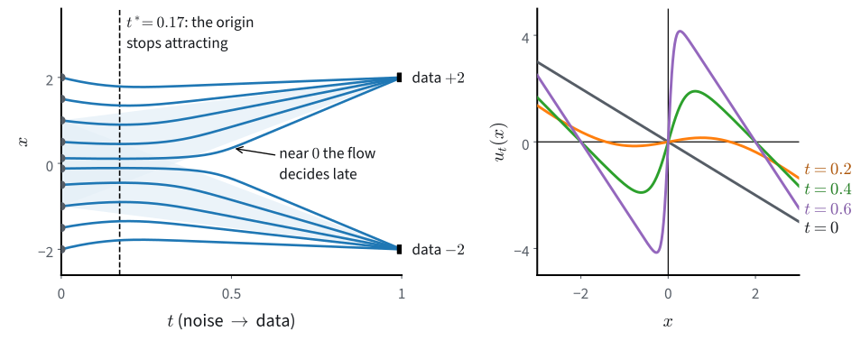
Does the closed form agree with a direct posterior average, where does the origin stop attracting, and where does one Euler step of the exact field land? The cell checks all three, the slope by a finite difference.
a = 2.0                                       # data at -a and +a, noise N(0, 1)
def u_two_point(x, t):                        # closed form of the marginal velocity
    return (a * np.tanh(t * a * x / (1 - t)**2) - x) / (1 - t)

def u_posterior(x, t):                        # posterior average of (x1 - x)/(1 - t)
    x1 = np.array([-a, a])
    w = np.exp(-(x - t * x1)**2 / (2 * (1 - t)**2))   # likelihood of x given x1
    return ((w * x1).sum() / w.sum() - x) / (1 - t)

points = [(0.5, 0.5), (0.3, -1.0), (0.8, 0.1)]
print('closed form - posterior average:',
      max(abs(u_two_point(x, t) - u_posterior(x, t)) for t, x in points))
ts = np.array([0.1, 0.2, 0.5])
print('slope at the origin at t = 0.1, 0.2, 0.5:',
      ((u_two_point(1e-6, ts) - u_two_point(-1e-6, ts)) / 2e-6).round(2),
      '   t* =', round(3 - 2 * np.sqrt(2), 4))
x0 = np.array([-1.0, 1.0])
print('one Euler step of length 1 from', x0, 'lands at', x0 + u_two_point(x0, 0.0))
closed form - posterior average: 1.7763568394002505e-15
slope at the origin at t = 0.1, 0.2, 0.5: [-0.56 0.31 14. ] t* = 0.1716
one Euler step of length 1 from [-1. 1.] lands at [0. 0.]The closed form matches the posterior average to rounding error, the slope at the origin changes sign between \(t = 0.1\) and \(t = 0.2\), and one Euler step from either start lands on \(0\), the data mean. This is the limit of the construction. The conditional paths are straight, but the marginal flow is curved, and one step collapses every sample onto the mean. The rest of the section asks how to pair noise with data so that the flow comes out straight.
29.6.1.4 Score, Noise, and Velocity
The previous section trained a network to predict the noise. Do we need a second training run to obtain a velocity? We do not. On a Gaussian path the score, the noise, the clean point and the velocity are affine functions of one posterior mean, so each determines the others. Condition on a data point and take the path
\[ \mathbf{x}_t = \alpha_t\, \mathbf{x}_1 + \sigma_t\, \boldsymbol{\epsilon}, \qquad \boldsymbol{\epsilon} \sim \mathcal{N}(\mathbf{0}, \mathbf{I}), \tag{29.6.5}\]
with smooth coefficients \((\alpha_t, \sigma_t)\), \((\alpha_0, \sigma_0) = (0, 1)\) and \((\alpha_1, \sigma_1) = (1, 0)\). The blob around \(\alpha_t \mathbf{x}_1\) has width \(\sigma_t\): at \(t = 0\) it is the noise, at \(t = 1\) the data point. The diffusion clock swaps the two boundary conditions.
The smallest case is Gaussian data \(x_1 \sim \mathcal{N}(0, s_1^2)\) in one dimension on the cosine path \(\alpha_t = \sin\frac{\pi t}{2}\), \(\sigma_t = \cos\frac{\pi t}{2}\). The marginal is \(\mathcal{N}(0, s_t^2)\) with \(s_t^2 = \alpha_t^2 s_1^2 + \sigma_t^2\), the score is \(-x/s_t^2\), and the velocity is \(u_t(x) = (\dot{s}_t/s_t)\, x\): a Gaussian cloud only stretches or shrinks (5). With \(s_1 = 2\) at \(t = \tfrac12\) we get \(s_t^2 = 2.5\), and a particle at \(x\) moves with velocity \(0.94\, x\). With \(s_1 = 1\) every \(p_t\) is the standard Gaussian and the cloud never moves: \(u \equiv 0\).
Proposition (score–velocity identity). For the Gaussian path Equation 29.6.5, at any \(t\) with \(\alpha_t, \sigma_t > 0\) and on \(\{p_t > 0\}\), the marginal velocity and the marginal score determine each other:
\[ \mathbf{u}_t(\mathbf{x}) = \frac{\dot{\alpha}_t}{\alpha_t}\, \mathbf{x} - \left( \sigma_t \dot{\sigma}_t - \sigma_t^2\, \frac{\dot{\alpha}_t}{\alpha_t} \right) \nabla \log p_t(\mathbf{x}). \tag{29.6.6}\]
The velocity is a multiple of the position plus a multiple of the score, and the schedule alone fixes both multiples.
Proof. We show that both sides are affine in one posterior mean, \(\hat{\mathbf{x}}_1 = \mathbb{E}[\mathbf{x}_1 \mid \mathbf{x}_t = \mathbf{x}]\). Differentiating the path gives the conditional velocity \(\dot{\mathbf{x}}_t = \dot{\alpha}_t \mathbf{x}_1 + \dot{\sigma}_t \boldsymbol{\epsilon}\), and \(\boldsymbol{\epsilon} = (\mathbf{x} - \alpha_t \mathbf{x}_1)/\sigma_t\). Taking the posterior mean as in Equation 29.6.2,
\[ \mathbf{u}_t(\mathbf{x}) = \frac{\dot{\sigma}_t}{\sigma_t}\, \mathbf{x} + \left( \dot{\alpha}_t - \alpha_t\, \frac{\dot{\sigma}_t}{\sigma_t} \right) \hat{\mathbf{x}}_1. \]
The marginal score is the posterior mean of the scores of the kernels, which is Tweedie’s formula of the previous section. The kernel \(\mathcal{N}(\alpha_t \mathbf{x}_1, \sigma_t^2 \mathbf{I})\) has score \((\alpha_t \mathbf{x}_1 - \mathbf{x})/\sigma_t^2\), so
\[ \nabla \log p_t(\mathbf{x}) = \mathbb{E}\left[ \frac{\alpha_t \mathbf{x}_1 - \mathbf{x}}{\sigma_t^2} \,\middle|\, \mathbf{x}_t = \mathbf{x} \right] = \frac{\alpha_t \hat{\mathbf{x}}_1 - \mathbf{x}}{\sigma_t^2}, \qquad \textrm{i.e.}\quad \hat{\mathbf{x}}_1 = \frac{\mathbf{x} + \sigma_t^2\, \nabla \log p_t(\mathbf{x})}{\alpha_t}. \]
Substituting this \(\hat{\mathbf{x}}_1\) into the velocity and collecting the \(\mathbf{x}\) and \(\nabla \log p_t\) terms gives Equation 29.6.6. \(\blacksquare\)
On a variance-preserving path, \(\alpha_t^2 + \sigma_t^2 = 1\), so \(\sigma_t \dot{\sigma}_t = -\alpha_t \dot{\alpha}_t\) and the coefficient of the score collapses to \(\dot{\alpha}_t/\alpha_t\): \(\mathbf{u}_t(\mathbf{x}) = \frac{\dot{\alpha}_t}{\alpha_t}\big(\mathbf{x} + \nabla \log p_t(\mathbf{x})\big)\). On the straight path \(\alpha_t = t\), \(\sigma_t = 1 - t\) the identity reads \(\mathbf{u}_t(\mathbf{x}) = \mathbf{x}/t + \frac{1 - t}{t}\, \nabla \log p_t(\mathbf{x})\). For the Gaussian example, \(\nabla \log p_t = -x/s_t^2\) turns the first form into \(\frac{\dot\alpha_t}{\alpha_t}(1 - 1/s_t^2)\, x = \alpha_t \dot{\alpha}_t (s_1^2 - 1)\, x / s_t^2\), the stretching rate \(\dot{s}_t/s_t\) found above.
The same posterior mean underlies the targets that networks are trained on in practice (Table 29.6.1).
| Network predicts | Posterior mean | From the score \(\mathbf{s} = \nabla \log p_t\) |
|---|---|---|
| score \(\mathbf{s}_{\boldsymbol{\theta}}\) | \(\nabla \log p_t(\mathbf{x})\) | \(\mathbf{s}\) |
| noise \(\hat{\boldsymbol{\epsilon}}\) | \(\mathbb{E}[\boldsymbol{\epsilon} \mid \mathbf{x}_t = \mathbf{x}]\) | \(-\sigma_t\, \mathbf{s}\) |
| clean point \(\hat{\mathbf{x}}_1\) | \(\mathbb{E}[\mathbf{x}_1 \mid \mathbf{x}_t = \mathbf{x}]\) | \((\mathbf{x} + \sigma_t^2\, \mathbf{s})/\alpha_t\) |
| velocity \(\mathbf{v}_{\boldsymbol{\theta}}\) | \(\mathbb{E}[\dot{\mathbf{x}}_t \mid \mathbf{x}_t = \mathbf{x}]\) | the identity Equation 29.6.6 |
| \(v\)-prediction \(\hat{\mathbf{v}}\) | \(\mathbb{E}[\alpha_t \boldsymbol{\epsilon} - \sigma_t \mathbf{x}_1 \mid \mathbf{x}_t = \mathbf{x}]\) | \(-\tfrac{\sigma_t}{\alpha_t}\, \mathbf{x} - \sigma_t\, \tfrac{\alpha_t^2 + \sigma_t^2}{\alpha_t}\, \mathbf{s}\) |
Each row is a \(t\)-dependent affine function of the same posterior mean, so a network trained on any row defines all of them. Which row is easiest to learn is a separate question, about the variance of the training targets at the two ends of the path (8).
We can check the identity on the running mixture, components at \(\pm 2\) with variance \(0.25\), without fitting any model. At one fixed time on the cosine path, the cell computes the velocity once from the posterior mean, with no score in sight, and once from Equation 29.6.6 with the analytic score.
t = 0.6                                       # one fixed time, cosine schedule
alpha, sigma = np.sin(np.pi * t / 2), np.cos(np.pi * t / 2)
dalpha, dsigma = np.pi / 2 * sigma, -np.pi / 2 * alpha
grid = np.linspace(-4.0, 4.0, 201)
means, var0 = np.array([-2.0, 2.0]), 0.25     # the running mixture
vart = alpha**2 * var0 + sigma**2             # noised component variance
w = np.stack([np.exp(-(grid - alpha * m)**2 / (2 * vart)) for m in means])
w /= w.sum(0)                                 # posterior mode responsibilities
x1_hat = (w * np.stack([m + alpha * var0 / vart * (grid - alpha * m)
                        for m in means])).sum(0)          # E[x_1 | x_t]
u_posterior = dalpha * x1_hat + dsigma / sigma * (grid - alpha * x1_hat)
score = (w * np.stack([(alpha * m - grid) / vart for m in means])).sum(0)
u_dictionary = (dalpha / alpha) * grid \
    - (sigma * dsigma - sigma**2 * dalpha / alpha) * score
print(f'max |u_posterior - u_dictionary| on [-4, 4]: '
      f'{np.abs(u_posterior - u_dictionary).max():.1e}')
max |u_posterior - u_dictionary| on [-4, 4]: 3.1e-15The two routes agree to about \(10^{-15}\), across both modes and the valley between them. A trained noise predictor is therefore also a velocity field, and the samplers of this section can run on it unchanged.
29.6.2 Rectified Flow
29.6.2.1 Straight Paths and Their Crossings
The two-point example used straight conditional paths. In \(d\) dimensions the same construction pairs a noise sample \(\mathbf{x}_0\) with a data sample \(\mathbf{x}_1\), drawn independently, and joins them by a straight line traversed at constant speed:
\[ \mathbf{x}_t = (1 - t)\, \mathbf{x}_0 + t\, \mathbf{x}_1, \qquad \mathbf{u}_t(\mathbf{x}_t \mid \mathbf{z}) = \dot{\mathbf{x}}_t = \mathbf{x}_1 - \mathbf{x}_0, \qquad \mathbf{z} = (\mathbf{x}_0, \mathbf{x}_1). \tag{29.6.7}\]
The conditional velocity does not depend on \(t\), and the CFM loss Equation 29.6.3 becomes the rectified flow objective (Liu et al. 2023; Lipman et al. 2023)
\[ \mathcal{L}_{\mathrm{RF}}(\boldsymbol{\theta}) = \mathbb{E}_{t,\ \mathbf{x}_0 \sim p_0,\ \mathbf{x}_1 \sim p_1} \left[\, \left\| \mathbf{v}_{\boldsymbol{\theta}}\big( (1 - t) \mathbf{x}_0 + t \mathbf{x}_1,\ t \big) - (\mathbf{x}_1 - \mathbf{x}_0) \right\|^2 \right]. \tag{29.6.8}\]
Training draws noise and data, interpolates between them, and regresses on the difference. Given \(\mathbf{z}\), a point sliding along a line has no density, so the proposition does not apply as stated. Its conclusion still holds, by the same computation applied to the expectation \(\mathbb{E}\,\varphi(\mathbf{x}_t)\) of a smooth test function \(\varphi\) (9). Gaussian conditional paths with general \((\alpha_t, \sigma_t)\) recover the diffusion targets of the previous section instead.
Although every conditional path is straight, the marginal flow is not (Figure 29.6.3). Two segments that cross at \((\mathbf{x}, t)\) feed the posterior mean Equation 29.6.2 two different directions. A function has one value at each point, so the field averages them. An ODE whose field is Lipschitz in \(\mathbf{x}\) has exactly one trajectory through each point (Section 29.1.1.4), so two trajectories of the learned flow can never meet. Where the segments cross, the trajectories bend away from each other instead.

The goal is a field whose trajectories are straight lines traversed at constant speed. Such a field is constant along each trajectory, so one Euler step of any length is exact. The independent pairing is far from this limit, as the two-point example already showed. The bend comes from the pairing and not from the loss, because every conditional path is already a straight line.
29.6.2.2 Example: Two Moons
The two moons are two interleaved crescents in the plane. One Euler step of the exact field would collapse the noise onto their mean, and we can count how many steps a trained field needs instead. To score samples we use the squared energy distance (Székely and Rizzo 2013) between laws \(P\) and \(Q\) with finite first moments,
\[ \mathcal{E}^2(P, Q) = 2\, \mathbb{E}\|X - Y\| - \mathbb{E}\|X - X'\| - \mathbb{E}\|Y - Y'\|, \]
where \(X, X' \sim P\) and \(Y, Y' \sim Q\) are independent. It compares the mean distance between a point of \(P\) and a point of \(Q\) with the mean distances within each law. It is the squared MMD of Section 28.3.3.2 with the kernel \(k(\mathbf{x}, \mathbf{y}) = \|\mathbf{x}\| + \|\mathbf{y}\| - \|\mathbf{x} - \mathbf{y}\|\), and it is zero only if \(P = Q\). We estimate it from two samples by the U-statistic, which divides each within-sample sum by the number \(n(n-1)\) of ordered pairs of distinct points, so that the estimate is unbiased.
The cell builds the data, standardized to zero mean and unit variance per coordinate, a held-out sample of \(2{,}048\) points, and one noise array z_eval that every later comparison reuses.
def two_moons(n, rng, noise=0.07):
    t = rng.uniform(0.0, np.pi, n)
    m = rng.integers(0, 2, n)                      # which moon
    X = np.stack([np.cos(t) * (1 - 2 * m) + m,
                  np.sin(t) * (1 - 2 * m) + 0.5 * m], axis=1)
    return X + noise * rng.standard_normal((n, 2))

rng = np.random.default_rng()
raw = two_moons(8192, rng)
mu, sd = raw.mean(0), raw.std(0)
moons = (raw - mu) / sd                            # standardized training data
held_out = (two_moons(2048, rng) - mu) / sd
z_eval = rng.standard_normal((2048, 2))            # noise for every comparison

def energy_distance(a, b):                         # squared energy distance, U-statistic
    d = lambda u, v: np.linalg.norm(u[:, None, :] - v[None, :, :], axis=-1)
    n, m = len(a), len(b)
    return (2 * d(a, b).mean() - d(a, a).sum() / (n * (n - 1))
            - d(b, b).sum() / (m * (m - 1)))

print(f'fresh data sample vs held-out: {energy_distance(moons[:2048], held_out):+.4f}')
print(f'point mass at the data mean vs held-out: '
f'{energy_distance(np.zeros((2048, 2)), held_out):.3f}')fresh data sample vs held-out: -0.0002
point mass at the data mean vs held-out: 0.906fresh data sample vs held-out: -0.0000
point mass at the data mean vs held-out: 0.909fresh data sample vs held-out: -0.0011
point mass at the data mean vs held-out: 0.909fresh data sample vs held-out: -0.0012
point mass at the data mean vs held-out: 0.909Two samples of the same law score within a few thousandths of zero, which is the resolution of the metric at this sample size. A point mass at the data mean, which is what one Euler step of the exact field produces, scores about \(0.9\).
The model is a velocity field \(\mathbf{v}_{\boldsymbol{\theta}} : \mathbb{R}^2 \times [0, 1] \to \mathbb{R}^2\), a \(3 \to 64 \to 64 \to 2\) tanh network with Glorot-uniform weights and zero biases. It is trained by Adam for \(4{,}000\) steps of \(256\) pairs, with a learning rate that falls from \(3 \times 10^{-3}\) to zero along a cosine. The decay keeps the final weights from jittering with the last few batches.
The function train_rf takes a sampler of pairs, so that we can reuse it with a different pairing later. It returns the network and the mean loss over the last \(500\) batches, because the loss of a single batch of \(256\) scatters by about \(\pm 0.1\). The code averages the squared error over the two coordinates, so the printed loss is \(\mathcal{L}_{\mathrm{RF}}/2\).
def make_net():                         # 3 -> 64 -> 64 -> 2, Glorot weights, zero biases
    net = nn.Sequential(nn.Linear(3, 64), nn.Tanh(), nn.Linear(64, 64), nn.Tanh(),
                        nn.Linear(64, 2))
    for layer in net[::2]:
        nn.init.xavier_uniform_(layer.weight)
        nn.init.zeros_(layer.bias)
    return net

def train_rf(sample_pairs, steps=4000, tail=500):
    """Regress v(x_t, t) on x1 - x0; return the net and the mean tail loss."""
    net = make_net()
    opt = torch.optim.Adam(net.parameters(), lr=3e-3)
    sched = torch.optim.lr_scheduler.CosineAnnealingLR(opt, steps)   # 3e-3 -> 0
    tail_sum = torch.zeros(())
    for step in range(steps):
        x0, x1 = sample_pairs(256)
        t = torch.rand(256, 1)
        xt = (1 - t) * x0 + t * x1                 # a point on each segment
        loss = ((net(torch.cat([xt, t], 1)) - (x1 - x0))**2).mean()
        opt.zero_grad()
        loss.backward()
        opt.step()
        sched.step()
        if step >= steps - tail:
            tail_sum += loss.detach()              # stays on the device
    return net, (tail_sum / tail).item()
def make_net(): # Dense: Glorot-uniform weights, zero biases
net = tf.keras.Sequential([tf.keras.layers.Dense(64, 'tanh'),
tf.keras.layers.Dense(64, 'tanh'),
tf.keras.layers.Dense(2)])
net.build((None, 3))
return net
def train_rf(sample_pairs, steps=4000, tail=500):
"""Regress v(x_t, t) on x1 - x0; return the net and the mean tail loss."""
net = make_net()
lr = tf.keras.optimizers.schedules.CosineDecay(3e-3, steps) # 3e-3 -> 0
opt = tf.keras.optimizers.Adam(lr)
@tf.function
def train_step():
x0, x1 = sample_pairs(256)
t = tf.random.uniform((256, 1))
xt = (1 - t) * x0 + t * x1 # a point on each segment
with tf.GradientTape() as tape:
loss = tf.reduce_mean((net(tf.concat([xt, t], 1)) - (x1 - x0))**2)
grads = tape.gradient(loss, net.trainable_variables)
opt.apply_gradients(zip(grads, net.trainable_variables))
return loss
tail_sum = tf.zeros(())
for step in range(steps):
loss = train_step()
if step >= steps - tail:
tail_sum += loss # stays on the device
return net, float(tail_sum) / taildef make_params(key, sizes=(3, 64, 64, 2)): # Glorot-uniform weights, zero biases
glorot = jax.nn.initializers.glorot_uniform()
keys = jax.random.split(key, len(sizes) - 1)
return [(glorot(k, (i, o)), jnp.zeros(o))
for k, i, o in zip(keys, sizes[:-1], sizes[1:])]
def mlp(params, x):
for W, b in params[:-1]:
x = jnp.tanh(x @ W + b)
W, b = params[-1]
return x @ W + b
def train_rf(sample_pairs, steps=4000, tail=500):
"""Regress v(x_t, t) on x1 - x0; return the parameters and the mean tail loss.
sample_pairs(key, n) draws n pairs."""
opt = optax.adam(optax.cosine_decay_schedule(3e-3, steps)) # 3e-3 -> 0
def loss_fn(params, key):
k_pairs, k_t = jax.random.split(key)
x0, x1 = sample_pairs(k_pairs, 256)
t = jax.random.uniform(k_t, (256, 1))
xt = (1 - t) * x0 + t * x1 # a point on each segment
return ((mlp(params, jnp.concatenate([xt, t], 1)) - (x1 - x0))**2).mean()
def step(carry, key):
params, state = carry
loss, grads = jax.value_and_grad(loss_fn)(params, key)
updates, state = opt.update(grads, state)
return (optax.apply_updates(params, updates), state), loss
k_init, k_steps = jax.random.split(jax.random.key(np.random.randint(2**31)))
params = make_params(k_init)
(params, _), losses = jax.lax.scan(step, (params, opt.init(params)),
jax.random.split(k_steps, steps))
return params, float(losses[-tail:].mean())def make_net(): # init.Xavier() is Glorot uniform; biases 0
net = gluon.nn.HybridSequential()
net.add(gluon.nn.Dense(64, activation='tanh'),
gluon.nn.Dense(64, activation='tanh'), gluon.nn.Dense(2))
net.initialize(init.Xavier())
net.hybridize()
return net
def train_rf(sample_pairs, steps=4000, tail=500):
"""Regress v(x_t, t) on x1 - x0; return the net and the mean tail loss."""
net = make_net()
lr = lr_scheduler.CosineScheduler(steps, base_lr=3e-3) # 3e-3 -> 0
trainer = gluon.Trainer(net.collect_params(), 'adam',
{'learning_rate': 3e-3, 'lr_scheduler': lr})
tail_sum = 0
for step in range(steps):
x0, x1 = sample_pairs(256)
t = mxnp.random.uniform(0, 1, (256, 1))
xt = (1 - t) * x0 + t * x1 # a point on each segment
with autograd.record():
loss = ((net(mxnp.concatenate([xt, t], axis=1)) - (x1 - x0))**2).mean()
loss.backward()
trainer.step(1)
if step >= steps - tail:
tail_sum = tail_sum + loss # stays on the device
return net, float(tail_sum) / tailWhere does the loss settle when noise and data are paired independently?
data = torch.tensor(moons, dtype=torch.float32)
def independent_pairs(n):                       # fresh noise, random data rows
    return torch.randn(n, 2), data[torch.randint(0, len(data), (n,))]

net, plateau = train_rf(independent_pairs)
print(f'CFM loss, mean of the last 500 batches: {plateau:.2f}')
CFM loss, mean of the last 500 batches: 1.44data = tf.constant(moons, tf.float32)
def independent_pairs(n): # fresh noise, random data rows
return (tf.random.normal((n, 2)),
tf.gather(data, tf.random.uniform((n,), 0, len(moons), tf.int32)))
net, plateau = train_rf(independent_pairs)
print(f'CFM loss, mean of the last 500 batches: {plateau:.2f}')CFM loss, mean of the last 500 batches: 1.44data = jnp.asarray(moons, dtype=jnp.float32)
def independent_pairs(key, n): # fresh noise, random data rows
k_noise, k_rows = jax.random.split(key)
return (jax.random.normal(k_noise, (n, 2)),
data[jax.random.randint(k_rows, (n,), 0, len(data))])
net, plateau = train_rf(independent_pairs)
print(f'CFM loss, mean of the last 500 batches: {plateau:.2f}')CFM loss, mean of the last 500 batches: 1.44data = mxnp.array(moons)
def independent_pairs(n): # fresh noise, random data rows
return mxnp.random.normal(0, 1, (n, 2)), data[mxnp.random.randint(0, len(data), (n,))]
net, plateau = train_rf(independent_pairs)
print(f'CFM loss, mean of the last 500 batches: {plateau:.2f}')CFM loss, mean of the last 500 batches: 1.44The loss settles at about \(1.4\) per coordinate and cannot go much lower. By the theorem it is bounded below by the floor \(C\), the conditional variance of \(\mathbf{x}_1 - \mathbf{x}_0\) given \(\mathbf{x}_t\), averaged over \(t\). For this data set the floor can be computed by weighting every training point by its posterior probability given \(\mathbf{x}_t\); it is \(1.38\) per coordinate (1), and the network sits a few hundredths above it. Almost all of the remaining loss is the disagreement of crossing segments, which no network can remove.
Sampling integrates \(\dot{\mathbf{x}} = \mathbf{v}_{\boldsymbol{\theta}}(\mathbf{x}, t)\) from \(t = 0\) to \(1\) with Euler’s method (Section 29.1.3). The function euler_path takes a NumPy array of starting points and returns the whole trajectory, of shape (steps + 1, n, 2), as a NumPy array; its last row is the sample.
@torch.inference_mode()
def euler_path(net, z, steps):
    q = torch.tensor(z, dtype=torch.float32)
    path = [q]
    for k in range(steps):
        t = torch.full((len(z), 1), k / steps)
        q = q + net(torch.cat([q, t], 1)) / steps
        path.append(q)
    return torch.stack(path).numpy()
def euler_path(net, z, steps):
q = tf.constant(z, tf.float32)
path = [q]
for k in range(steps):
t = tf.fill((len(z), 1), k / steps)
q = q + net(tf.concat([q, t], 1)) / steps
path.append(q)
return tf.stack(path).numpy()def euler_path(params, z, steps):
def step(q, t):
q = q + mlp(params, jnp.concatenate([q, jnp.full((len(z), 1), t)], 1)) / steps
return q, q
q0 = jnp.asarray(z, dtype=jnp.float32)
_, path = jax.lax.scan(step, q0, jnp.arange(steps) / steps)
return np.concatenate([np.asarray(q0)[None], np.asarray(path)])def euler_path(net, z, steps):
q = mxnp.array(z, dtype='float32')
path = [q]
for k in range(steps):
t = mxnp.full((len(z), 1), k / steps)
q = q + net(mxnp.concatenate([q, t], axis=1)) / steps
path.append(q)
return mxnp.stack(path).asnumpy()How does the quality of the samples depend on the number of Euler steps? The cell integrates the same noise array z_eval with \(K = 1, 2, \ldots, 64\) steps and plots the energy distance to the held-out data on log–log axes.
steps_list = [1, 2, 4, 8, 16, 32, 64]
eds = [energy_distance(euler_path(net, z_eval, K)[-1], held_out) for K in steps_list]
print('  '.join(f'{K}: {e:.3f}' for K, e in zip(steps_list, eds)))
d2l.plot(steps_list, eds, 'Euler steps', 'squared energy distance',
xscale='log', yscale='log')1: 0.633 2: 0.147 4: 0.034 8: 0.008 16: 0.002 32: 0.001 64: 0.001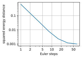
1: 0.674 2: 0.141 4: 0.034 8: 0.008 16: 0.003 32: 0.001 64: 0.001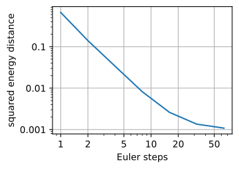
1: 0.633 2: 0.148 4: 0.036 8: 0.009 16: 0.003 32: 0.001 64: 0.001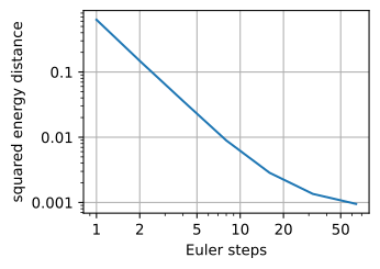
1: 0.643 2: 0.141 4: 0.034 8: 0.009 16: 0.004 32: 0.003 64: 0.003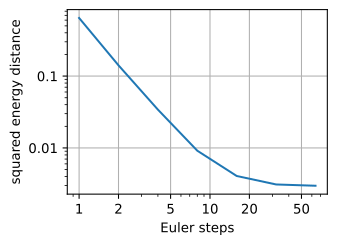
One step scores between \(0.6\) and \(0.7\), the same order as the point mass at the mean (\(0.9\)): the network has learned, imperfectly, the collapse that the exact field performs at \(t = 0\). Two steps score about \(0.15\), four about \(0.04\), eight about \(0.01\), and from sixteen steps on the score levels off, usually at a few thousandths and never much above \(0.01\). The decline is Euler’s discretization error. The level that remains is the error of the trained field; it varies with the training run and is often as small as the metric can resolve with \(2{,}048\) points. The samples show the same progression.
fig, axes = d2l.plt.subplots(1, 4, figsize=(10, 2.6), sharex=True, sharey=True)
for ax, K in zip(axes, (1, 2, 8, 32)):
    s = euler_path(net, z_eval, K)[-1]
    d2l.plot(s[:, 0], s[:, 1], f'{K} Euler step(s)', fmts=('.',),
             xlim=(-2.5, 2.5), ylim=(-2.5, 2.5), axes=ax)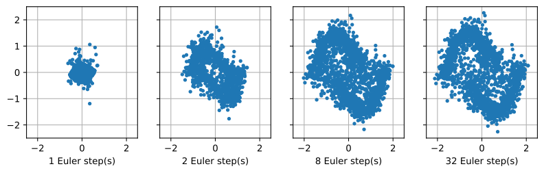
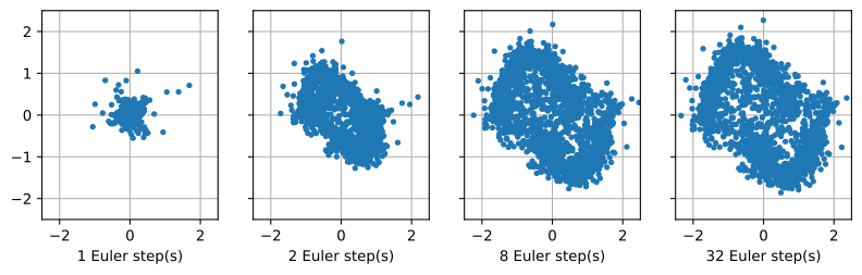
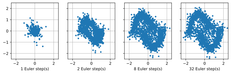
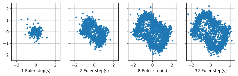
One step gives a blob around the mean, two a bent ellipse, eight recognizable moons, and thirty-two sharp ones. The curvature that the independent pairing builds into the flow costs sixteen to thirty-two network calls per sample.
29.6.2.3 Reflow
The independent pairing is what bends the flow, and the trained model supplies a better one. Run its ODE from fresh noise and pair each start \(\mathbf{x}_0\) with the endpoint \(\hat{\mathbf{x}}_1(\mathbf{x}_0)\) that it produced. Trajectories of one flow never cross, so these pairs cross far less than independent ones. Retraining the same architecture on the new pairs is called reflow (Liu et al. 2023). It keeps both endpoint distributions and does not increase the cost of transport, for every convex cost function.
Proposition (reflow keeps the marginals and lowers the transport cost). Let \((\mathbf{X}_0, \mathbf{X}_1) \sim \pi\) have finite second moments, let \(\mathbf{X}_t = (1 - t) \mathbf{X}_0 + t \mathbf{X}_1\), let \(\mathbf{u}_t\) be the marginal velocity of this straight path, and let \(\mathbf{Z}_t\) solve \(\dot{\mathbf{Z}}_t = \mathbf{u}_t(\mathbf{Z}_t)\) from \(\mathbf{Z}_0 = \mathbf{X}_0\). Assume that \(\mathbf{X}_t\) has a positive density for every \(t < 1\) and that \(\mathbf{u}_t\) is continuously differentiable and Lipschitz in \(\mathbf{x}\) with a constant independent of \(t\), so that this flow exists. Then (i) \(\mathbf{Z}_t\) has the law of \(\mathbf{X}_t\) for every \(t\), in particular \(\mathbf{Z}_1 \sim p_1\); (ii) for every convex function \(c\),
\[ \mathbb{E}\, c(\mathbf{Z}_1 - \mathbf{Z}_0) \;\le\; \mathbb{E}\, c(\mathbf{X}_1 - \mathbf{X}_0). \tag{29.6.9}\]
Proof. (i) The law of \(\mathbf{X}_t\) satisfies the continuity equation with \(\mathbf{u}_t\), by the marginal-velocity proposition with \(\mathbf{z} = (\mathbf{X}_0, \mathbf{X}_1)\) in the weak form that covers point masses (9). The law of \(\mathbf{Z}_t\) satisfies it too, because \(\mathbf{Z}_t\) moves with the field \(\mathbf{u}_t\). Both start from \(p_0\), and two solutions of the continuity equation with such a field that start equal stay equal: along each trajectory both log-densities change at the rate \(-\nabla \cdot \mathbf{u}_t\). This is the argument that gave the probability-flow ODE its marginals in Section 29.4.4.3. (ii) Write the displacement as a time integral and apply Jensen’s inequality twice:
\[ \mathbb{E}\, c(\mathbf{Z}_1 - \mathbf{Z}_0) = \mathbb{E}\, c\Big(\int_0^1 \mathbf{u}_t(\mathbf{Z}_t)\, dt\Big) \le \int_0^1 \mathbb{E}\, c\big(\mathbf{u}_t(\mathbf{Z}_t)\big)\, dt = \int_0^1 \mathbb{E}\, c\big(\mathbb{E}[\mathbf{X}_1 - \mathbf{X}_0 \mid \mathbf{X}_t]\big)\, dt \le \mathbb{E}\, c(\mathbf{X}_1 - \mathbf{X}_0). \]
The first inequality is Jensen’s inequality for the time average. The equality uses (i) to replace \(\mathbf{Z}_t\) by \(\mathbf{X}_t\) and then the definition of the marginal velocity. The last inequality is the conditional Jensen inequality. \(\blacksquare\)
With \(c = \|\cdot\|^2\) the last step loses exactly the conditional variance, so the cost falls at least by the floor of the old pairing: \(\mathbb{E}\|\mathbf{Z}_1 - \mathbf{Z}_0\|^2 \le \mathbb{E}\|\mathbf{X}_1 - \mathbf{X}_0\|^2 - C\). Re-pairing helps only where segments cross, because there the conditional velocity is not a function of \((\mathbf{x}_t, t)\).
The two points show the effect in closed form. A flow in one dimension preserves order, so one round pairs each \(x_0\) with \(a \operatorname{sign}(x_0)\) (6). This pairing costs \(a^2 - 2a\sqrt{2/\pi} + 1 = 1.81\) against \(a^2 + 1 = 5\) for the independent one, and its segments never cross, so the second round has \(C = 0\) and its field is integrated exactly by one Euler step.
For the two moons, the cell draws \(8{,}192\) fresh noise points, integrates the trained model for \(32\) steps to obtain their endpoints, and trains a new network with train_rf on these fixed pairs.
x0_pairs = np.random.standard_normal((8192, 2))      # noise endpoints, kept
x1_pairs = euler_path(net, x0_pairs, 32)[-1]          # the model's own endpoints
X0, X1 = (torch.tensor(p, dtype=torch.float32) for p in (x0_pairs, x1_pairs))
def model_pairs(n):                                   # the same pairs, never re-paired
    i = torch.randint(0, len(X0), (n,))
    return X0[i], X1[i]

net2, plateau2 = train_rf(model_pairs)
print(f'reflow loss, mean of the last 500 batches: {plateau2:.4f}')
reflow loss, mean of the last 500 batches: 0.0044x0_pairs = np.random.standard_normal((8192, 2)) # noise endpoints, kept
x1_pairs = euler_path(net, x0_pairs, 32)[-1] # the model's own endpoints
X0, X1 = (tf.constant(p, tf.float32) for p in (x0_pairs, x1_pairs))
def model_pairs(n): # the same pairs, never re-paired
i = tf.random.uniform((n,), 0, len(x0_pairs), tf.int32)
return tf.gather(X0, i), tf.gather(X1, i)
net2, plateau2 = train_rf(model_pairs)
print(f'reflow loss, mean of the last 500 batches: {plateau2:.4f}')reflow loss, mean of the last 500 batches: 0.0040x0_pairs = np.random.standard_normal((8192, 2)) # noise endpoints, kept
x1_pairs = euler_path(net, x0_pairs, 32)[-1] # the model's own endpoints
X0, X1 = jnp.asarray(x0_pairs, jnp.float32), jnp.asarray(x1_pairs, jnp.float32)
def model_pairs(key, n): # the same pairs, never re-paired
i = jax.random.randint(key, (n,), 0, len(X0))
return X0[i], X1[i]
net2, plateau2 = train_rf(model_pairs)
print(f'reflow loss, mean of the last 500 batches: {plateau2:.4f}')reflow loss, mean of the last 500 batches: 0.0035x0_pairs = np.random.standard_normal((8192, 2)) # noise endpoints, kept
x1_pairs = euler_path(net, x0_pairs, 32)[-1] # the model's own endpoints
X0, X1 = mxnp.array(x0_pairs), mxnp.array(x1_pairs)
def model_pairs(n): # the same pairs, never re-paired
i = mxnp.random.randint(0, len(x0_pairs), (n,))
return X0[i], X1[i]
net2, plateau2 = train_rf(model_pairs)
print(f'reflow loss, mean of the last 500 batches: {plateau2:.4f}')reflow loss, mean of the last 500 batches: 0.0043The reflow loss settles at a few thousandths instead of \(1.4\), so the new segments almost never cross. How does this change sampling, and how far did the pairing cost drop? The next cell compares the two models from the same noise array and prints the mean squared length of the old and the new pairs.
for K in (1, 2, 32):
    e1 = energy_distance(euler_path(net, z_eval, K)[-1], held_out)
    e2 = energy_distance(euler_path(net2, z_eval, K)[-1], held_out)
    print(f'{K:2d} Euler step(s): energy distance  original {e1:.3f}  reflowed {e2:.3f}')
x1_indep = moons[np.random.randint(0, len(moons), len(x0_pairs))]
print(f'mean squared pair length: independent {np.mean(np.sum((x1_indep - x0_pairs)**2, 1)):.2f}'
f', reflowed {np.mean(np.sum((x1_pairs - x0_pairs)**2, 1)):.2f}') 1 Euler step(s): energy distance original 0.633 reflowed 0.001
2 Euler step(s): energy distance original 0.147 reflowed 0.001
32 Euler step(s): energy distance original 0.001 reflowed 0.002
mean squared pair length: independent 3.93, reflowed 0.28 1 Euler step(s): energy distance original 0.674 reflowed 0.001
2 Euler step(s): energy distance original 0.141 reflowed 0.002
32 Euler step(s): energy distance original 0.001 reflowed 0.002
mean squared pair length: independent 3.95, reflowed 0.27 1 Euler step(s): energy distance original 0.633 reflowed 0.002
2 Euler step(s): energy distance original 0.148 reflowed 0.002
32 Euler step(s): energy distance original 0.001 reflowed 0.002
mean squared pair length: independent 4.09, reflowed 0.28 1 Euler step(s): energy distance original 0.643 reflowed 0.003
2 Euler step(s): energy distance original 0.141 reflowed 0.003
32 Euler step(s): energy distance original 0.003 reflowed 0.003
mean squared pair length: independent 3.86, reflowed 0.27One Euler step of the reflowed model scores the same as thirty-two steps of the original, usually a few thousandths, and about a hundred times below the original’s single step. The reflowed network was trained to reproduce the original’s \(32\)-step endpoints, so matching their quality in one step is the best it can do. It inherits the first model’s error.
The mean squared length of the pairs drops from \(4\) to about \(0.3\). For the exact marginal flow the proposition guarantees a drop at least to \(4 - 2.76 = 1.24\), since the floor of the independent pairing is \(2 \times 1.38 = 2.76\) summed over the two coordinates. The trained network and its \(32\) Euler steps only approximate that flow, and the measured drop is far larger than the bound. The first step of the proof, Jensen’s inequality for the time average, is far from tight on the curved trajectories of the first flow.
Are the reflowed trajectories straight? The cell measures the mean distance of each \(32\)-step trajectory from the chord joining its two ends.
def chord_gap(P):                                     # P: (steps + 1, n, 2) trajectory
    chord = P[0] + (P[-1] - P[0]) * np.linspace(0, 1, len(P))[:, None, None]
    return np.linalg.norm(P - chord, axis=-1).mean()

print(f'mean distance from the chord: original {chord_gap(euler_path(net, z_eval, 32)):.3f}'
f', reflowed {chord_gap(euler_path(net2, z_eval, 32)):.3f}')mean distance from the chord: original 0.244, reflowed 0.017mean distance from the chord: original 0.245, reflowed 0.015mean distance from the chord: original 0.242, reflowed 0.016mean distance from the chord: original 0.248, reflowed 0.017The original trajectories wander about a quarter of a unit from their chords, first toward the mean as the two-point example predicts and then out to the moons. The reflowed ones stay within about two hundredths, which is why one step suffices. Reflow straightens a flow, but it does not make it optimal. In more than one dimension a flow can be crossing-free and still move mass farther than it must, as we show next.
29.6.3 Optimal Transport and Straightness
29.6.3.1 Couplings and the Wasserstein Distance
Reflow lowered the transport cost. Which pairing is cheapest, and is its flow straight? Section 28.3.3.3 set up the vocabulary, which we restate. A coupling \(\pi\) of \(p_0\) and \(p_1\) is a joint law of pairs with these marginals, a plan that says how much mass travels from each source point to each target point. The 2-Wasserstein distance is the cost of the cheapest plan under squared distance,
\[ W_2^2(p_0, p_1) = \min_{\pi \in \Pi(p_0, p_1)}\ \mathbb{E}_{(\mathbf{x}_0, \mathbf{x}_1) \sim \pi} \left[\, \| \mathbf{x}_1 - \mathbf{x}_0 \|^2 \right], \tag{29.6.10}\]
where \(\Pi(p_0, p_1)\) is the set of couplings. The distance is the least mean squared distance by which the mass must move. When \(p_0\) has a density and both laws have finite second moments, the optimal plan is unique and is a map, \(\mathbf{x}_1 = \nabla \psi(\mathbf{x}_0)\) for a convex function \(\psi\). This is Brenier’s theorem (Brenier 1991).
The smallest case is a Gaussian in one dimension, from \(\mathcal{N}(0, 1)\) to \(\mathcal{N}(m, s^2)\) with \(s > 0\). The sorted pairing sends each quantile to the same quantile, \(x_1 = m + s x_0\), and costs \(\mathbb{E}(m + s x_0 - x_0)^2 = m^2 + (s - 1)^2\). The independent pairing costs \(\mathbb{E}(x_1 - x_0)^2 = m^2 + 1 + s^2\). In one dimension the sorted pairing is optimal for every convex cost: if two pairs cross, swapping their targets does not increase the cost (4). Hence
\[ W_2^2\big(\mathcal{N}(0, 1), \mathcal{N}(m, s^2)\big) = m^2 + (s - 1)^2 . \tag{29.6.11}\]
The distance separates the cost of shifting the mean from the cost of stretching the width. From \(\mathcal{N}(0, 1)\) to \(\mathcal{N}(0, 4)\) it is \(1\), against \(5\) for independent pairs: the independent pairing spends four fifths of its cost moving mass past other mass.
This explains where the trajectories of Figure 29.6.3 end. In one dimension the trajectories of a flow cannot cross, so a flow preserves order, and the order-preserving pairing is the optimal one. On a line, one round of reflow therefore reaches optimal transport (6).
In two dimensions, freedom from crossings is not enough. Rotate a standard Gaussian cloud about the origin by a quarter turn in unit time, with the field that assigns to the point \((\xi_1, \xi_2)\) the velocity \(\tfrac{\pi}{2}\, (-\xi_2, \xi_1)\). No two trajectories cross, and the cloud ends where it started, so \(W_2^2(p_0, p_1) = 0\). Yet every particle moves, at speed \(\tfrac{\pi}{2}\|\mathbf{x}\|\). The cost of a whole flow, not only of its endpoints, is its kinetic energy \(\int_0^1 \mathbb{E}\|\mathbf{u}_t(\mathbf{x}_t)\|^2\, dt\), the mean squared speed of the particles integrated over time. For the rotation it is \((\pi/2)^2\, \mathbb{E}\|\mathbf{x}\|^2 = \pi^2/2 \approx 4.9\). On a line, crossings are the only way to waste motion; in the plane a flow can also waste it by turning (Figure 29.6.4).
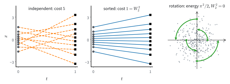
Kinetic energy also ranks flows with the same endpoints. Which of three flows between \(\mathcal{N}(0, 1)\) and \(\mathcal{N}(0, 4)\) costs least: the straight flow of the sorted pairing, the marginal flow of straight segments under the independent pairing, or the cosine path with data \(\mathcal{N}(0, 4)\) from the score–velocity subsection? All three have Gaussian marginals \(\mathcal{N}(0, s_t^2)\), so their velocity is \((\dot{s}_t/s_t)\, x\) and the kinetic energy is \(\int_0^1 \dot{s}_t^2\, dt\) (5). The cell also checks the two pairing costs by sorting samples.
n = 200_000
x0, x1 = np.random.standard_normal(n), 2 * np.random.standard_normal(n)
print(f'N(0,1) -> N(0,4): independent pairing {np.mean((x1 - x0)**2):.2f}, '
      f'sorted pairing {np.mean((np.sort(x1) - np.sort(x0))**2):.3f}')
t = np.linspace(0, 1, 100_001)
def kinetic_energy(s):                       # marginals N(0, s_t^2): u_t(x) = (s'/s) x
    return np.sum(np.diff(s)**2 / np.diff(t))  # the integral of (ds/dt)^2

for name, s in [('sorted, straight', 1 + t),
                ('independent, straight', np.sqrt((1 - t)**2 + 4 * t**2)),
                ('cosine path', np.sqrt(1 + 3 * np.sin(np.pi * t / 2)**2))]:
print(f'{name:22s} kinetic energy {kinetic_energy(s):.3f}')N(0,1) -> N(0,4): independent pairing 5.03, sorted pairing 1.012
sorted, straight kinetic energy 1.000
independent, straight kinetic energy 1.858
cosine path kinetic energy 1.234N(0,1) -> N(0,4): independent pairing 4.99, sorted pairing 0.994
sorted, straight kinetic energy 1.000
independent, straight kinetic energy 1.858
cosine path kinetic energy 1.234N(0,1) -> N(0,4): independent pairing 4.99, sorted pairing 0.998
sorted, straight kinetic energy 1.000
independent, straight kinetic energy 1.858
cosine path kinetic energy 1.234N(0,1) -> N(0,4): independent pairing 5.00, sorted pairing 1.007
sorted, straight kinetic energy 1.000
independent, straight kinetic energy 1.858
cosine path kinetic energy 1.234The sorted straight flow attains \(W_2^2 = 1\). The straight segments of the independent pairing produce a marginal flow that costs \(1.86\), more than the cosine path’s \(1.23\). Its width \(s_t^2 = (1 - t)^2 + 4t^2\) first shrinks, until \(t = 0.2\), and then grows, so its particles move inward and back out. Straight conditional segments under the wrong pairing do not make a straight flow.
29.6.3.2 The Benamou–Brenier Theorem
The last cell compared flows by their kinetic energy, and the cheapest one reached \(W_2^2\). This is a general fact. It connects the static problem Equation 29.6.10, which pairs endpoints, to the objects that flow matching trains, which are flows.
Theorem (Benamou–Brenier). Let \(p_0\) have a density, let \(p_0\) and \(p_1\) have finite second moments, and call a pair \((p_t, \mathbf{u}_t)\) admissible if \(\mathbf{u}_t\) is continuously differentiable and Lipschitz in \(\mathbf{x}\) with a constant independent of \(t\), and the pair satisfies the continuity equation with the endpoints \(p_0\) and \(p_1\). Every admissible pair has kinetic energy at least \(W_2^2(p_0, p_1)\). If the straight interpolation of an optimal coupling has an admissible marginal velocity (for example, when the Brenier map is a smooth diffeomorphism whose derivative and inverse derivative are bounded), that flow has kinetic energy \(W_2^2\), so (Benamou and Brenier 2000)
\[ W_2^2(p_0, p_1) = \min_{(p_t, \mathbf{u}_t)}\ \int_0^1 \int \| \mathbf{u}_t(\mathbf{x}) \|^2\, p_t(\mathbf{x})\, d\mathbf{x}\, dt . \tag{29.6.12}\]
The squared Wasserstein distance is the least kinetic energy of any flow carrying \(p_0\) to \(p_1\).
Proof. The proof sandwiches the kinetic energy between \(W_2^2\) from below and from above.
I. Every flow defines a coupling. Let \(\mathbf{X}_t\) solve \(\dot{\mathbf{X}}_t = \mathbf{u}_t(\mathbf{X}_t)\) from \(\mathbf{X}_0 \sim p_0\). By the uniqueness fact used in the reflow proposition, \(\mathbf{X}_t \sim p_t\) for every \(t\), so \((\mathbf{X}_0, \mathbf{X}_1)\) is a coupling of \(p_0\) and \(p_1\).
- Lower bound. The cost of this coupling is at least \(W_2^2\), and Jensen’s inequality for the time average bounds it by the kinetic energy:
\[ W_2^2(p_0, p_1) \le \mathbb{E} \left\| \mathbf{X}_1 - \mathbf{X}_0 \right\|^2 = \mathbb{E} \left\| \int_0^1 \mathbf{u}_t(\mathbf{X}_t)\, dt \right\|^2 \le \int_0^1 \mathbb{E} \left\| \mathbf{u}_t(\mathbf{X}_t) \right\|^2 dt = \int_0^1\!\! \int \|\mathbf{u}_t\|^2\, p_t\, d\mathbf{x}\, dt . \]
- Upper bound. Take an optimal coupling \(\pi^\star\) and its straight interpolation \(\mathbf{X}_t = (1 - t)\mathbf{X}_0 + t\mathbf{X}_1\), with marginal velocity \(\mathbf{u}_t(\mathbf{x}) = \mathbb{E}[\mathbf{X}_1 - \mathbf{X}_0 \mid \mathbf{X}_t = \mathbf{x}]\). By the marginal-velocity proposition in its weak form this pair satisfies the continuity equation with the right endpoints, and by the conditional Jensen inequality its kinetic energy is
\[ \int_0^1 \mathbb{E}\big\|\mathbb{E}[\mathbf{X}_1 - \mathbf{X}_0 \mid \mathbf{X}_t]\big\|^2\, dt \le \mathbb{E}\|\mathbf{X}_1 - \mathbf{X}_0\|^2 = W_2^2(p_0, p_1). \]
The two bounds meet. \(\blacksquare\)
When the field that flow matching would learn on an optimal coupling is admissible, it is the minimizer. Since the lower bound also applies to it, the inequality in III is an equality, so the conditional variance is zero: the segments of an optimal coupling do not cross. Jensen’s inequality in II is tight only if each particle moves at constant velocity, so every minimizer moves its particles along straight lines at constant speed. A straight constant-speed flow attains \(W_2^2\) only if, in addition, its pairing is optimal. The straight interpolation between each \(\mathbf{x}_0\) and its quarter turn \(\mathbf{R}\mathbf{x}_0\) (9) is straight, crossing-free and not optimal.
29.6.3.3 Approximate Optimal Couplings
The probability-flow trajectories of diffusion are curved, and for a fixed pairing curvature raises the kinetic energy. Curvature does not by itself fix the number of solver steps, which also depends on the solver and on how fast the field varies. Reflow re-pairs by the model and never raises the cost, as the proposition shows. A minibatch optimal-transport pairing (Tong et al. 2024; Pooladian et al. 2023) re-pairs each batch of \(256\) noise and data points by the assignment of least total squared distance before training. On the two moons this lowers the loss plateau from \(1.4\) to about \(0.06\) per coordinate and the one-step energy distance to a few thousandths (7). Neither method finds the optimal coupling of the marginals: a batch plan depends on the batch, and reflow inherits the errors of the first model.
29.6.4 Sampling with a Learned Field
29.6.4.1 Deterministic and Stochastic Samplers
A trained network is a score \(\mathbf{s}_{\boldsymbol{\theta}}\) or a velocity \(\mathbf{v}_{\boldsymbol{\theta}}\), and generating a sample means integrating the dynamics it defines. A velocity is integrated forward on the flow-matching clock. A score is integrated on the diffusion clock, with forward drift \(\mathbf{f}\) and diffusion coefficient \(g\), by the probability-flow ODE of Section 29.4.4.3 or the reverse SDE of Section 29.4.5:
\[ \underbrace{\dot{\mathbf{x}} = \mathbf{v}_{\boldsymbol{\theta}}(\mathbf{x}, t) \quad \textrm{or} \quad \dot{\mathbf{x}} = \mathbf{f} - \tfrac{1}{2} g^2\, \mathbf{s}_{\boldsymbol{\theta}}}_{\textrm{deterministic (ODE)}} \qquad \textrm{versus} \qquad \underbrace{d\mathbf{x} = \left[ \mathbf{f} - g^2\, \mathbf{s}_{\boldsymbol{\theta}} \right] dt + g\, d\bar{\mathbf{W}}}_{\textrm{stochastic (reverse SDE)}}, \]
where \(\bar{\mathbf{W}}\) is a Brownian motion run backward in time. The two score samplers share the drift \(\mathbf{f}\). The SDE doubles the score term and adds noise, and the two changes balance so that both have the same marginals. Both are integrated by the solvers of Section 29.1.3 and Section 29.3.4.1.
The ODE is deterministic, so one starting point gives one sample. The trace integral of Section 29.2.3 gives the log-density of the model’s own flow, up to solver and trace-estimation error, and it equals the data density only when the learned field is exact. The SDE injects fresh noise at every step, and the number of steps it needs is tuned separately from that of the ODE.
29.6.4.2 Solver Order at Equal Cost
The cost of a sample is the number of field evaluations (NFE). Heun’s method is second order but evaluates the field twice per step. Is it worth two evaluations? To isolate the discretization error from the learning error, we use the probability-flow ODE with the exact score of the running mixture, components at \(\pm 2\) with variance \(0.25\), under the variance-preserving schedule with \(\beta(t)\) rising linearly from \(0.1\) to \(20\). The cell integrates from \(t = 1\) to \(t = 0\) on the diffusion clock with Euler and with Heun’s method (Section 29.1.3), and compares the endpoints of \(8{,}000\) starting points with a Heun solution of \(800\) steps. Both methods get the same budgets of \(10\) to \(80\) evaluations, spent on two grids of times: equal steps in \(t\), and the squared grid \(t_k = u_k^2\) with \(u_k\) equally spaced from \(1\) to \(0\), whose steps shrink toward the data end \(t = 0\).
bmin, bmax = 0.1, 20.0
beta_fn = lambda t: bmin + t * (bmax - bmin)            # VP noise schedule
abar_fn = lambda t: np.exp(-(bmin * t + 0.5 * (bmax - bmin) * t**2))
def score_vp(q, t, means=(-2.0, 2.0), var=0.25):        # exact mixture score
    a = abar_fn(t)
    v = a * var + (1 - a)
    w = np.stack([np.exp(-(q - np.sqrt(a) * m)**2 / (2 * v)) for m in means])
    return (w * np.stack([(np.sqrt(a) * m - q) / v
                          for m in means])).sum(0) / w.sum(0)
def pf_ode(q, t):                                       # probability-flow ODE
    return -0.5 * beta_fn(t) * (q + score_vp(q, t))
def solve(q, ts, heun=False):                           # steps along grid ts
    for t1, t2 in zip(ts[:-1], ts[1:]):
        h, d1 = t2 - t1, pf_ode(q, t1)
        q = q + 0.5 * h * (d1 + pf_ode(q + h * d1, t2)) if heun else q + h * d1
    return q
grids = {'uniform': lambda K: np.linspace(1, 0, K + 1),     # equal steps in t
         'squared': lambda K: np.linspace(1, 0, K + 1)**2}  # dense near t = 0
z = np.random.default_rng(0).standard_normal(8000)
ref = solve(z, grids['uniform'](800), heun=True)        # fine reference
nfes = [10, 20, 40, 80]                                 # Heun: n // 2 steps
errs = {f'{m}, {g}': [np.abs(solve(z, grid(n // k), k == 2) - ref).mean()
                      for n in nfes]
        for g, grid in grids.items() for m, k in (('Euler', 1), ('Heun', 2))}
print(f'{"NFE":16s}' + ''.join(f'{n:8d}' for n in nfes))
for name, e in errs.items():
    print(f'{name:16s}' + ''.join(f'{v:8.4f}' for v in e))
d2l.plot(nfes, list(errs.values()), 'field evaluations', 'mean endpoint error',
legend=list(errs), xscale='log', yscale='log')NFE 10 20 40 80
Euler, uniform 0.0419 0.0194 0.0095 0.0047
Heun, uniform 0.0784 0.0276 0.0083 0.0023
Euler, squared 0.1057 0.0518 0.0256 0.0127
Heun, squared 0.0329 0.0143 0.0045 0.0012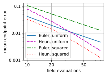
NFE                   10      20      40      80
Euler, uniform    0.0419  0.0194  0.0095  0.0047
Heun, uniform     0.0784  0.0276  0.0083  0.0023
Euler, squared    0.1057  0.0518  0.0256  0.0127
Heun, squared     0.0329  0.0143  0.0045  0.0012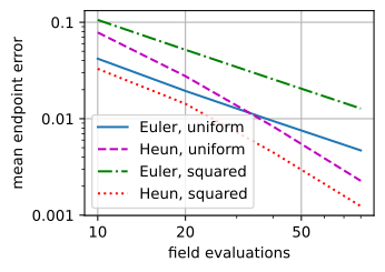
NFE                   10      20      40      80
Euler, uniform    0.0419  0.0194  0.0095  0.0047
Heun, uniform     0.0784  0.0276  0.0083  0.0023
Euler, squared    0.1057  0.0518  0.0256  0.0127
Heun, squared     0.0329  0.0143  0.0045  0.0012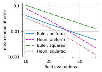
NFE                   10      20      40      80
Euler, uniform    0.0419  0.0194  0.0095  0.0047
Heun, uniform     0.0784  0.0276  0.0083  0.0023
Euler, squared    0.1057  0.0518  0.0256  0.0127
Heun, squared     0.0329  0.0143  0.0045  0.0012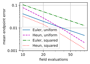
On the uniform grid the orders show in the rates. Each doubling of the budget divides Euler’s error by about two and Heun’s by a factor that grows toward four (\(2.8\), \(3.3\), \(3.6\)). At equal cost, though, Heun loses at \(10\) evaluations (about \(0.08\) against Euler’s \(0.04\)) and at \(20\) (\(0.028\) against \(0.02\)), and leads only from \(40\). On the squared grid Heun wins at every budget, and at \(10\) evaluations its error, about \(0.03\), is below Euler’s on either grid. Euler moves the other way: the squared grid more than doubles its error. Where the steps go matters more than the order of the solver.
The shape of the paths explains this. Until about \(t = 0.5\) the noised law is close to \(\mathcal{N}(0, 1)\), whose score \(-x\) cancels the drift, so the field is nearly zero and the paths cover less than a tenth of their length. They then speed up toward their modes, fastest near \(t = 0.25\), where the samples that start between the modes commit to one of them, and slow down as they settle. The error of each step, carried forward to \(t = 0\), has a sign that depends on where the step lies. Euler moves with the velocity at the start of a step, so it falls short while the paths speed up and overshoots while they slow down. Heun’s step acts like the trapezoid rule for the velocity. It overshoots where the speed curves upward, above about \(t = 0.4\), falls short where it curves downward, between about \(t = 0.1\) and \(0.4\), and is nearly exact near \(t = 0\), where the speed falls almost linearly.
The endpoint error is what remains after these signed errors cancel. On the uniform grid Euler’s shortfalls and overshoots are about equal, and they cancel to about an eighth of their total size at every budget. Heun’s errors are mostly shortfalls, because its overshoots come from the stretch where the field is nearly zero, so little cancels. The squared grid changes the total size of the step errors little, by about a tenth for Euler and less for Heun, but it changes their balance. Its longer early steps and shorter late steps shrink Euler’s overshoots, so Euler loses its cancellation. For Heun the same grid enlarges the overshoots and shrinks the shortfalls, and its error halves. The steep parts of the field play little part: the slope at the origin reaches about \(-33\) at \(t = 0.1\), but by then the paths have left the origin, and near \(t = 1\) the large \(\beta\) multiplies a field that is nearly zero.
Diffusion samplers crowd their steps toward the data as well, and choose how much by measurement. EDM (Karras et al. 2022) spaces its noise levels so that \(\sigma_i^{1/\rho}\) is equally spaced from \(\sigma_{\max}^{1/\rho}\) to \(\sigma_{\min}^{1/\rho}\), which crowds the steps at low noise as the squared grid crowds them near \(t = 0\). Its authors report that \(\rho = 3\) nearly equalizes the local errors of the steps, yet \(\rho\) between \(5\) and \(10\) samples images better, and they use \(\rho = 7\). Paired with Heun’s method, this grid samples \(32 \times 32\) images in \(35\) evaluations. The grid and the solver are chosen together, and the best grid depends on the schedule and on the data.
29.6.4.3 Comparison of Model Families
The methods of this section and the previous one differ in the path they fix, the quantity they regress on, and the solver they sample with.
| Model family | Object learned | Training loss | Sampler | Stochastic? |
|---|---|---|---|---|
| DDPM (Ho et al. 2020) | noise \(\boldsymbol{\epsilon}_{\boldsymbol{\theta}}(\mathbf{x}_t, t)\), a rescaled score | \(\mathbb{E} \lVert \boldsymbol{\epsilon} - \boldsymbol{\epsilon}_{\boldsymbol{\theta}} \rVert^2\), denoising score matching with weight \(w(t) = \sigma_t^2\) | ancestral reverse chain of about \(1000\) steps | yes |
| Score SDE (Y. Song et al. 2021) | score \(\mathbf{s}_{\boldsymbol{\theta}}(\mathbf{x}, t)\) | the noise-conditional denoising score matching loss of the previous section | reverse SDE by Euler–Maruyama | yes |
| Probability-flow ODE (Y. Song et al. 2021) | the same \(\mathbf{s}_{\boldsymbol{\theta}}\) | the same | ODE solver; log-density of the model’s own flow by the trace integral | no |
| DDIM (J. Song et al. 2021) | the same \(\boldsymbol{\epsilon}_{\boldsymbol{\theta}}\) as DDPM | the same as DDPM | the deterministic DDIM update of the previous section on a sparse time grid | no |
| Flow matching, rectified flow (Lipman et al. 2023; Liu et al. 2023) | velocity \(\mathbf{v}_{\boldsymbol{\theta}}(\mathbf{x}, t)\) | CFM Equation 29.6.3; on the straight path, regression on \(\mathbf{x}_1 - \mathbf{x}_0\) | ODE solver | no |
Every row regresses onto a conditional mean of a closed-form per-sample quantity, and samples with a solver from this chapter.
We can now learn a score or a velocity from samples by one regression and convert either into the other on a Gaussian path. We can read the cost of a flow from its kinetic energy, and integrate any of these fields with the solvers of Section 29.1, choosing the solver and its time grid together. What remains open is the pairing of noise with data. Independent pairs make the flow curve, and reflow and batch re-pairing straighten it on the two moons. No known method finds the optimal pairing cheaply in high dimension, and the number of steps a learned field needs is still found by trial. Chapter 17 takes up both questions for images.
29.6.5 Summary
A probability path from noise to data can be chosen freely. The velocity that realizes it is the posterior mean of the velocities of per-sample paths, so conditional flow matching trains it by least squares, with the same gradients as the intractable marginal loss. On a Gaussian path the velocity and the score are affine in one posterior mean, so one network can be read as either. On straight conditional paths the marginal flow bends wherever segments cross. Reflow re-pairs noise with the model’s own endpoints, does not increase the transport cost, and straightens the flow: one Euler step of the reflowed two-moons model matches thirty-two steps of the original. The squared Wasserstein distance is the least kinetic energy of any flow between the endpoints, attained by straight constant-speed motion under an optimal pairing. Sampling is numerical integration, and where the steps go matters more than the order of the solver: on a uniform grid Heun’s method loses to Euler below about \(40\) evaluations, and on a grid crowded toward the data it wins at every budget.
29.6.6 Exercises
- Crossing segments and the floor. The constant \(C\) of the CFM theorem is the conditional variance \(\mathbb{E} \| Y - \mathbf{u}_t(\mathbf{x}) \|^2\) of the target \(Y = \mathbf{u}_t(\mathbf{x} \mid \mathbf{z})\).
- Show that \(C = 0\) if and only if, for almost every \(t\), the conditional velocity is almost surely a function of \((\mathbf{x}_t, t)\). What does this require of the segments of the straight path Equation 29.6.7?
- For the independent pairing of \(\mathcal{N}(\mathbf{0}, \mathbf{I})\) with the standardized
moons, compute the conditional variance of \(\mathbf{x}_1 - \mathbf{x}_0\) given \(\mathbf{x}_t\), summed over coordinates, at \(t = 0\) and at \(t = 1\). The training cell prints the loss per coordinate; which number should it be compared with? - Compute the floor numerically. Draw \((t, \mathbf{x}_0, \mathbf{x}_1)\), form \(\mathbf{x}_t\), weight every training point \(\mathbf{x}_1'\) by \(\exp\big(-\|\mathbf{x}_t - t\mathbf{x}_1'\|^2 / 2(1 - t)^2\big)\), and average the posterior variance of \(\mathbf{x}_1\), divided by \((1 - t)^2\), over a few thousand draws. Compare the result with the printed plateau. At which \(t\) is the per-\(t\) floor largest, and why does it fall toward both ends?
- The reflow loss settles at a few thousandths. What does this say about crossings among the segments from \(\mathbf{x}_0\) to \(\hat{\mathbf{x}}_1(\mathbf{x}_0)\), allowing for the approximation error of the network?
- Stochastic interpolants. ● Albergo et al. (2023) write the paths of this section and of the previous one as \(\mathbf{x}_t = a_t \mathbf{x}_0 + b_t \mathbf{x}_1 + c_t \mathbf{w}\), where \((\mathbf{x}_0, \mathbf{x}_1)\) is drawn from a coupling of \(p_0\) and \(p_1\), \(\mathbf{w} \sim \mathcal{N}(\mathbf{0}, \mathbf{I})\) is independent of both, and the smooth schedules satisfy \(a_0 = b_1 = 1\) and \(a_1 = b_0 = c_0 = c_1 = 0\). With a Gaussian \(p_0\) the diffusion and rectified-flow paths are the one-sided case \(c \equiv 0\); the latent term \(c_t \mathbf{w}\) serves two-sided paths between arbitrary \(p_0\) and \(p_1\).
- Take \(\mathbf{z} = (\mathbf{x}_0, \mathbf{x}_1, \mathbf{w})\) in the marginal velocity Equation 29.6.2. Show that it is \(\mathbb{E}[\dot{a}_t \mathbf{x}_0 + \dot{b}_t \mathbf{x}_1 + \dot{c}_t \mathbf{w} \mid \mathbf{x}_t = \mathbf{x}]\), and write the corresponding CFM loss Equation 29.6.3.
- Give schedules that recover rectified flow Equation 29.6.7 and the cosine path, whose data and noise coefficients are \(\sin \tfrac{\pi t}{2}\) and \(\cos \tfrac{\pi t}{2}\), both with independent endpoints and \(p_0 = \mathcal{N}(\mathbf{0}, \mathbf{I})\).
- For \(p_0 = \mathcal{N}(\mathbf{0}, \mathbf{I})\), independent endpoints, and \(c_t > 0\), show that the interpolant has the same marginal velocity as the interpolant with \(c \equiv 0\) and \(\sqrt{a_t^2 + c_t^2}\) in place of \(a_t\).
- For \(c_t > 0\), show that \(\nabla \log p_t(\mathbf{x}) = -\mathbb{E}[\mathbf{w} \mid \mathbf{x}_t = \mathbf{x}] / c_t\). What does interior noise provide when \(p_0\) is an arbitrary data distribution rather than a Gaussian?
- Late decisions. Take the two-point example with data \(\pm a\).
- Derive Equation 29.6.4 from the posterior over \(x_1\), and show that the terms in \(x^2\) cancel in the log-odds.
- Show that \(\partial_x u_t(0) = \big(t a^2/(1 - t)^2 - 1\big)/(1 - t)\) and that the origin turns from attracting to repelling at \(t^* = \tfrac12\big(2 + a^2 - \sqrt{(2 + a^2)^2 - 4}\big)\), which is \(3 - 2\sqrt{2} \approx 0.17\) for \(a = 2\). How does \(t^*\) behave as \(a \to \infty\) and as \(a \to 0\)? Interpret both limits.
- Show that away from the origin the slope \(\partial_x u_t\) tends to \(-1/(1 - t)\), and that an Euler step of length \(h\) from \(t = 1 - h\) lands exactly on \(\pm a\) from any point where the \(\tanh\) is saturated. Which part of the flow, then, limits a fixed-step solver, and at which times?
- Show that \(C = \mathbb{E}_t \mathbb{E}_x \textrm{Var}(x_1 \mid x_t)/(1 - t)^2\) is finite although the conditional velocity \((x_1 - x)/(1 - t)\) is unbounded. Use \(\textrm{Var}(x_1 \mid x_t = x) = a^2 \operatorname{sech}^2\big(t a x/(1 - t)^2\big)\) and the fact that the density of \(x_t\) near \(0\) is of order \(e^{-t^2 a^2/2(1 - t)^2}/(1 - t)\).
- [code] Optimal transport in one dimension.
- For \(\mathcal{N}(0, 1) \to \mathcal{N}(m, s^2)\) with \(s > 0\), show that the sorted pairing is \(x_1 = m + s x_0\) and costs \(m^2 + (s - 1)^2\), while the independent pairing costs \(m^2 + 1 + s^2\).
- Prove that in one dimension the sorted pairing minimizes \(\mathbb{E}\, c(x_1 - x_0)\) for every convex \(c\). Suppose two pairs \((x_0, x_1)\) and \((x_0', x_1')\) cross: \(x_0 < x_0'\) but \(x_1 > x_1'\). Show that \(c(x_1' - x_0) + c(x_1 - x_0') \le c(x_1 - x_0) + c(x_1' - x_0')\). (The two new differences lie between the two old ones and have the same sum.) Conclude Equation 29.6.11.
- Show that the time-one map of a one-dimensional flow with a Lipschitz field is increasing, and hence that a flow carrying \(p_0\) to \(p_1\), with \(p_0\) a density, induces the sorted pairing. Conclude that in one dimension every such flow has an optimal pairing.
- Check (a) by sorting \(10^5\) samples for \((m, s) = (0, 2)\) and \((1, 2)\).
- [code] Kinetic energy of Gaussian paths.
- Show that if \(p_t = \mathcal{N}(0, s_t^2)\) in one dimension, the velocity \(u_t(x) = (\dot{s}_t/s_t)\, x\) satisfies the continuity equation, and that its kinetic energy is \(\int_0^1 \dot{s}_t^2\, dt\). Why does a Gaussian cloud need no other velocity?
- For \(\mathcal{N}(0, 1) \to \mathcal{N}(0, 4)\), find \(s_t\) for (i) the straight flow of the sorted pairing, (ii) the marginal flow of straight segments under the independent pairing, and (iii) the cosine path. Compute the three kinetic energies in closed form or by quadrature, and order them against \(W_2^2 = 1\).
- Explain why (ii) costs more than (iii) although its conditional segments are straight. Sketch \(s_t\) for both.
- Repeat (ii) for \(\mathcal{N}(0, 1) \to \mathcal{N}(0, 1)\). Show that the independent pairing has kinetic energy about \(0.43\) although \(W_2^2 = 0\). Which pairing costs nothing, and what is its flow?
- [code] One reflow round on two points. Take data \(\pm a\), noise \(\mathcal{N}(0, 1)\), the independent pairing, and the marginal flow Equation 29.6.4 of the two-point example.
- Using part (c) of 4, show that the time-one map is \(x_0 \mapsto a \operatorname{sign}(x_0)\), so one reflow round produces the sorted pairing.
- Show that its cost is \(a^2 - 2a\sqrt{2/\pi} + 1\), about \(1.81\) for \(a = 2\), against \(a^2 + 1 = 5\) for the independent pairing, and explain why this cost is \(W_2^2\).
- Show that the reflowed segments \((1 - t)\, x_0 + t\, a \operatorname{sign}(x_0)\) never cross, so that the floor of the second round is \(C = 0\), and write down its field. Is one Euler step of it exact?
- Integrate the closed-form field with RK4 from \(20{,}000\) Gaussian draws to \(t = 1 - 10^{-3}\) (the velocity grows like \(1/(1 - t)\), so stop short of \(1\)), and check the endpoints and the cost.
- The floor of the independent pairing is \(C \approx 2.03\) for \(a = 2\) (compute it). Check the bound \(\mathbb{E}\|\mathbf{Z}_1 - \mathbf{Z}_0\|^2 \le \mathbb{E}\|\mathbf{X}_1 - \mathbf{X}_0\|^2 - C\) of the reflow proposition. How much slack does it leave here?
- [code] Minibatch optimal-transport pairing. Replace
independent_pairsby a sampler that draws \(256\) noise points and \(256\) data points and re-pairs them by the assignment of least total squared distance (scipy.optimize.linear_sum_assignmenton the \(256 \times 256\) cost matrix), and train withtrain_rf.- Report the loss plateau, the energy distance at \(1\), \(2\), \(8\) and \(32\) steps, and the mean squared pair length before and after re-pairing. Compare with the independent pairing and with reflow.
- Show that a re-paired noise point is still a standard Gaussian draw and a re-paired data point is still a draw from the data, so the marginal field still carries \(p_0\) to \(p_1\).
- Explain why the batch pairing is not an optimal coupling of the two distributions, and what happens as the batch size grows. Which of the two re-pairing methods needs a trained model, and which inherits its errors?
- Conditioning of prediction targets. Take the Gaussian path Equation 29.6.5 with one-dimensional data \(x_1 \sim \mathcal{N}(0, 1)\) and the cosine path.
- Compute, as functions of \(t\), the variances of the sampled training targets in Table 29.6.1: the conditional score \(-\epsilon/\sigma_t\), the noise \(\epsilon\), the clean point \(x_1\), the velocity \(\dot{\alpha}_t x_1 + \dot{\sigma}_t \epsilon\), and the \(v\)-target \(\alpha_t \epsilon - \sigma_t x_1\). Which blow up, and at which end of the path?
- A network trained on the noise outputs \(\hat{\epsilon}\) with error \(\delta\). Show that the implied clean point \((x - \sigma_t \hat{\epsilon})/\alpha_t\) carries the error \(\sigma_t \delta/\alpha_t\), and that the noise implied by a clean-point prediction with error \(\delta\) carries \(\alpha_t \delta/\sigma_t\). At which end of the path is each amplified?
- Show that on the cosine path the velocity target equals \(-\pi/2\) times the \(v\)-target, so that \(v\)-prediction is velocity prediction, and that the velocity implied by a noise prediction carries the error \(\pi\delta/(2\alpha_t)\). Which parameterizations keep the error bounded at both ends?
- Reflow preserves marginals and can stall.
- Prove part (i) of the reflow proposition in detail for the straight path, whose conditional laws are point masses. For a smooth test function \(\varphi\) with compact support, show that \(\frac{d}{dt}\mathbb{E}\,\varphi(\mathbf{X}_t) = \mathbb{E}\big[\nabla\varphi(\mathbf{X}_t) \cdot \mathbf{u}_t(\mathbf{X}_t)\big]\), which is the continuity equation in weak form. Where is the tower property used, and where the Lipschitz hypothesis?
- Let \(\pi_k\) be the pairing after \(k\) rounds. Show that \(\mathbb{E}_{\pi_k}\|\mathbf{x}_1 - \mathbf{x}_0\|^2\) is non-increasing and bounded below by \(W_2^2\), hence convergent.
- Show that if a round changes nothing, \(\pi_{k+1} = \pi_k\), then \(C = 0\) for \(\pi_k\). Identify the fixed point in one dimension.
- In two dimensions pair each \(\mathbf{x}_0 \sim \mathcal{N}(\mathbf{0}, \mathbf{I})\) with \(\mathbf{R}\mathbf{x}_0\), where \(\mathbf{R}\) is the quarter-turn rotation. Show that the segments \(\big((1 - t)\mathbf{I} + t\mathbf{R}\big)\mathbf{x}_0\) never cross (the matrix is invertible for every \(t\), because its eigenvalues are \((1 - t) \pm \mathrm{i}\, t\)), so that \(C = 0\) and reflow changes nothing, while the cost is \(\mathbb{E}\|\mathbf{R}\mathbf{x}_0 - \mathbf{x}_0\|^2 = 4\) against \(W_2^2 = 0\). Which property beyond being straight and crossing-free does optimality need?
- [code] A stochastic sampler for a flow-matching model. ●
- On the straight path \(\alpha_t = t\), \(\sigma_t = 1 - t\), invert Equation 29.6.6 to get \(\nabla \log p_t(\mathbf{x}) = \big(t\, \mathbf{u}_t(\mathbf{x}) - \mathbf{x}\big)/(1 - t)\).
- Show that for every \(g \ge 0\) the SDE \(d\mathbf{X} = \big[\mathbf{u}_t(\mathbf{X}) + \tfrac12 g^2 \nabla \log p_t(\mathbf{X})\big] dt + g\, d\mathbf{W}\) has the marginals \(p_t\). Write its Fokker–Planck equation and use \(\nabla \cdot (p \nabla \log p) = \Delta p\). A trained velocity field therefore defines a family of stochastic samplers.
- Implement the sampler with Euler–Maruyama for the trained two-moons field, with \(g \in \{0, \tfrac12, 1\}\) and \(K \in \{8, 32, 128\}\) steps. Stop at \(t = 1 - 1/K\), because the score grows like \(1/(1 - t)\), and report the energy distance of each run. Which \(g\) needs the fewest steps for a given quality, and does noise help at \(K = 8\)?
- Repeat for the reflowed field. Explain, from the straightness of its trajectories, why no one-step stochastic sample can match its one-step deterministic sample.