%matplotlib inline
from d2l import torch as d2l
import math
import numpy as np
import time
import torch
from torch import nn12.2 Linear Recurrence and State Space Models
The gated cells of Section 12.1 improve information retention, but a recurrent network must consume its input one step at a time: \(\mathbf{H}_t\) cannot be computed before \(\mathbf{H}_{t-1}\) exists, so a sequence of length \(T\) costs \(T\) sequential rounds of work no matter how many processors we own. Modern accelerators are throughput machines, built to run tens of thousands of threads at once, and a recurrence at inference batch sizes leaves nearly all of them idle. Compare the convolutional networks of Chapter 6: a convolution applies the same weights at every position, just as a recurrence applies the same cell at every step, but all positions are computed at once. That difference in training throughput is what pushed recurrent networks out of large-scale use, far more than any difference in modeling power.
This section develops parallel evaluation while retaining a state of fixed size, updated in constant time per token at inference (Section 8.4.2.1). The nonlinearity in the state update prevents an associative evaluation. First we reduce the GRU down to a minimal gated cell whose update is linear in the state, which makes the whole sequence computable by a parallel scan in logarithmic depth. We then derive the linear recurrence from a continuous-time state space model (SSM): discretization provides step-size gates, a stable parameterization, an exact equivalence between recurrence and convolution, and, through the HiPPO theory, a principled answer to what dynamics make a fixed-size state a good memory of the past. The result is the S4 family of models (Gu, Goel, et al. 2022), the backbone of the selective state space models we meet in the next section and of recurrent layers inside several production language models.
Prerequisites: the gated cells and language-modeling recipe of Section 12.1, the gradient analysis of Section 8.6.2.1, and, for the classifier experiment, Fashion-MNIST from Section 3.2.
%matplotlib inline
from d2l import jax as d2l
from flax import nnx
import jax
from jax import numpy as jnp
import math
import numpy as np
import optax
import time
12.2.1 Linearizing the Recurrence
Why exactly can a recurrence not be parallelized? Take the vanilla update \(\mathbf{H}_t = \phi(\mathbf{X}_t \mathbf{W}_{\textrm{xh}} + \mathbf{H}_{t-1} \mathbf{W}_{\textrm{hh}} + \mathbf{b})\) and try to jump ahead two steps: substituting the update into itself buries \(\mathbf{H}_{t-2}\) under two nested applications of \(\phi\), and nothing simplifies. A composition of nonlinear maps has no compact closed form, so the only way to evaluate step \(t\) is to have evaluated step \(t-1\). The nonlinearity in the state path prevents this parallel evaluation. Gates computed from the input, nonlinear state readouts, and deep stacks of layers do not create the same dependency.
That observation suggests a surgical experiment: keep the gating idea of Section 12.1, but remove every appearance of \(\mathbf{H}_{t-1}\) inside a nonlinearity. Recall the GRU update, Equation 12.1.6 through Equation 12.1.8: two gates and a candidate, each a function of \(\mathbf{X}_t\) and \(\mathbf{H}_{t-1}\), followed by a convex blend. Feng et al. (2024) asked how much of that machinery is load-bearing and arrived at the minGRU by making two cuts. First, the update gate is computed from the input alone. Second, the candidate state is computed from the input alone, which leaves the reset gate with nothing to reset, so it is deleted outright. What survives is
\[ \mathbf{Z}_t = \sigma(\mathbf{X}_t \mathbf{W}_{\textrm{xz}} + \mathbf{b}_\textrm{z}), \qquad \tilde{\mathbf{H}}_t = \tanh(\mathbf{X}_t \mathbf{W}_{\textrm{xh}} + \mathbf{b}_\textrm{h}), \tag{12.2.1}\]
\[ \mathbf{H}_t = (1 - \mathbf{Z}_t) \odot \mathbf{H}_{t-1} + \mathbf{Z}_t \odot \tilde{\mathbf{H}}_t. \tag{12.2.2}\]
Here \(\mathbf{Z}_t\) gates the write, so \(\mathbf{Z}_t \approx 0\) means “hold the state”; substituting \(\mathbf{Z}_t \leftarrow 1 - \mathbf{Z}_t\) recovers the orientation of Equation 12.1.8. (Feng et al. also drop the \(\tanh\) on the candidate; we keep it because a bounded candidate trains more stably under the plain SGD recipe we reuse below, and an exercise asks you to remove it.) The cell looks almost unchanged, but its character is transformed: for fixed inputs, Equation 12.2.2 is an affine function of \(\mathbf{H}_{t-1}\),
\[ \mathbf{H}_t = \mathbf{a}_t \odot \mathbf{H}_{t-1} + \mathbf{b}_t, \qquad \mathbf{a}_t = 1 - \mathbf{Z}_t, \quad \mathbf{b}_t = \mathbf{Z}_t \odot \tilde{\mathbf{H}}_t, \tag{12.2.3}\]
where every coefficient \(\mathbf{a}_t, \mathbf{b}_t\) depends only on \(\mathbf{X}_t\) and hence can be computed for all \(t\) simultaneously, in one batched matrix product. Two consequences follow, and they organize the rest of this section. Parallelism: affine maps compose into affine maps, so the \(T\)-step recurrence can be evaluated by a divide-and-conquer scheme rather than a left-to-right walk. Analyzable memory: unrolling Equation 12.2.3 shows that the input from \(k\) steps ago reaches \(\mathbf{H}_t\) scaled by exactly \(\prod_{j=t-k+1}^{t} \mathbf{a}_j\), a product of gate values you can print, plot, and reason about. Because \(\mathbf{a}_t = 1 - \mathbf{Z}_t \in (0, 1)\) elementwise, that product can never explode, and how fast it decays is a learned, per-unit property: the eigenvalue analysis of Section 8.6.2.1 applies with the eigenvalues in plain sight. Linear recurrent units (LRUs) push the same idea further with complex-valued decays and careful initialization, and match well-tuned nonlinear RNNs on long-range benchmarks (Orvieto et al. 2023).
Does linearity in the state cost us expressivity? Within a single layer, yes: a linear state can only accumulate and forget, not compute. The answer, as everywhere else in deep learning, is depth: nonlinearities remain between layers, where they do not obstruct parallelism, and the stack recovers the lost capacity. We will see the pattern concretely in the S4D block near the end of this section.
12.2.2 Parallel Scans
12.2.2.1 An Associative Combine
The classic prefix sum problem asks for all running totals \(s_t = x_1 + \cdots + x_t\) of a sequence. It looks as sequential as our recurrence, yet it parallelizes beautifully, because addition is associative: sums may be grouped arbitrarily, so partial sums of blocks can be computed independently and merged. Blelloch (1990) showed the general result: a running “total” under any associative binary operator can be computed in \(O(\log T)\) parallel rounds. The operation is called a parallel scan, and it is exactly as general as it sounds.
Our recurrence fits once we find the right operator. Represent the affine update at step \(t\) by its coefficient pair \((\mathbf{a}_t, \mathbf{b}_t)\), standing for the map \(\mathbf{h} \mapsto \mathbf{a}_t \odot \mathbf{h} + \mathbf{b}_t\). Applying \((\mathbf{a}_1, \mathbf{b}_1)\) first and \((\mathbf{a}_2, \mathbf{b}_2)\) second gives \(\mathbf{a}_2 \odot (\mathbf{a}_1 \odot \mathbf{h} + \mathbf{b}_1) + \mathbf{b}_2\), which is again affine:
\[ (\mathbf{a}_2, \mathbf{b}_2) \circ (\mathbf{a}_1, \mathbf{b}_1) = (\mathbf{a}_1 \odot \mathbf{a}_2,\ \mathbf{a}_2 \odot \mathbf{b}_1 + \mathbf{b}_2). \tag{12.2.4}\]
The operator \(\circ\) is associative because function composition is associative, and composing the first \(t\) pairs yields the map that carries \(\mathbf{h}_0\) all the way to \(\mathbf{h}_t\); with \(\mathbf{h}_0 = \mathbf{0}\) the state is simply the \(\mathbf{b}\)-component of that composite. So the entire trajectory \(\mathbf{h}_1, \ldots, \mathbf{h}_T\) is the prefix scan of \((\mathbf{a}_1, \mathbf{b}_1), \ldots, (\mathbf{a}_T, \mathbf{b}_T)\) under Equation 12.2.4.
Figure 12.2.1 shows the parallel schedule we will implement, on eight elements. In round one, every position combines with its immediate predecessor; in round two, with the position two back; then four back, and so on, doubling the stride. After round \(r\) position \(t\) holds the composite of elements \(\max(1, t - 2^r + 1)\) through \(t\), so after \(\lceil \log_2 T \rceil\) rounds every position holds its full prefix. Each round is one batched elementwise multiply-add over the whole sequence, perfect work for an accelerator.
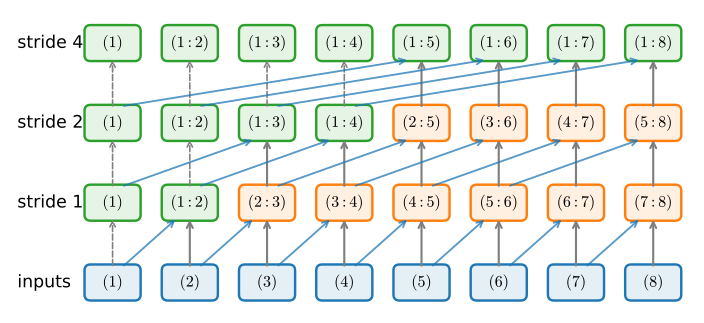
This doubling schedule is the scheme of Hillis and Steele: it performs \(O(T \log T)\) total work, a \(\log T\) factor more than the sequential loop, in exchange for \(O(\log T)\) depth. Blelloch’s classic two-sweep scan reduces the work to \(O(T)\) at slightly more than twice the depth and is common in production kernels. We use the Hillis–Steele form because its shorter implementation exposes the associative operation; its additional logarithmic work must be included when interpreting the timings below.
12.2.2.2 Implementation
We implement the doubling scan for the elementwise-affine recurrence \(\mathbf{h}_t = \mathbf{a}_t \odot \mathbf{h}_{t-1} + \mathbf{b}_t\) with \(\mathbf{h}_0 = \mathbf{0}\). Time runs along the first axis; any batch or feature axes ride along elementwise, and the coefficient tensors follow ordinary broadcasting rules, a convenience we will lean on later when \(\mathbf{a}\) is shared across the batch. Each iteration of the loop is one round of Figure 12.2.1: positions \(t < s\) keep their values (the [:s] prefix), and every other position combines with the value at stride \(s\) by Equation 12.2.4. The function is built from differentiable tensor ops, so gradients flow through training without further ado.
We save the helper in the d2l library: it is the computational core of this section and the next.
JAX ships the scan as a primitive: jax.lax.associative_scan takes the combine function and applies it in log depth. We only need to supply Equation 12.2.4 on (a, b) pairs.
def associative_scan(a, b, dim=0):
    """Parallel prefix scan for h_t = a_t * h_{t-1} + b_t with h_0 = 0."""
    a, b = a.movedim(dim, 0), b.movedim(dim, 0)
    step = 1
    while step < b.shape[0]:  # ceil(log2 T) rounds of combines
        a_prev, b_prev = a[:-step], b[:-step]
        a, b = (torch.cat([a[:step], a_prev * a[step:]]),
                torch.cat([b[:step], a[step:] * b_prev + b[step:]]))
        step *= 2
    return b.movedim(0, dim)
def scan_combine(prev, cur):
a_prev, b_prev = prev
a_cur, b_cur = cur
return a_prev * a_cur, a_cur * b_prev + b_cur
def associative_scan(a, b):
"""Parallel prefix scan for h_t = a_t * h_{t-1} + b_t with h_0 = 0."""
return jax.lax.associative_scan(scan_combine, (a, b))[1]Correctness first: on random coefficients (decays \(\mathbf{a}_t\) drawn in \((0, 1)\), a deliberately awkward length that is not a power of two), the scan must agree with the sequential loop it replaces.
def sequential_scan(a, b):
    h, outputs = d2l.zeros_like(b[0]), []
    for t in range(b.shape[0]):
        h = a[t] * h + b[t]
        outputs.append(h)
    return d2l.stack(outputs, 0)

a, b = torch.rand(100, 4, 8), torch.randn(100, 4, 8)
err = (associative_scan(a, b) - sequential_scan(a, b)).abs().max()
print(f'maximum deviation: {float(err):.2e}')
maximum deviation: 4.77e-07def sequential_scan(a, b):
step = lambda h, ab: (ab[0] * h + ab[1],) * 2
return jax.lax.scan(step, jnp.zeros_like(b[0]), (a, b))[1]
key1, key2 = jax.random.split(d2l.get_key())
a = jax.random.uniform(key1, (100, 4, 8))
b = jax.random.normal(key2, (100, 4, 8))
err = jnp.abs(associative_scan(a, b) - sequential_scan(a, b)).max()
print(f'maximum deviation: {float(err):.2e}')maximum deviation: 4.77e-07We time the parallel scan against the sequential evaluation as the sequence grows from 256 to 16,384 steps, at a fixed batch of 32 sequences with 128 units.
device = d2l.try_gpu()

def wall_clock(f, *args, reps=3):
    f(*args)  # Warm up
    if device.type == 'cuda':
        torch.cuda.synchronize()
    start = time.time()
    for _ in range(reps):
        f(*args)
    if device.type == 'cuda':
        torch.cuda.synchronize()
    return (time.time() - start) / reps

lengths, times = [256, 1024, 4096, 16384], [[], []]
for T in lengths:
    a = torch.rand(T, 32, 128, device=device)
    b = torch.randn(T, 32, 128, device=device)
    times[0].append(wall_clock(associative_scan, a, b) * 1e3)
    times[1].append(wall_clock(sequential_scan, a, b) * 1e3)
d2l.plot(lengths, times, 'sequence length', 'time per call (ms)',
         legend=['parallel scan', 'sequential loop'],
         xscale='log', yscale='log', figsize=(5, 3))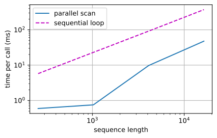
parallel_fn = jax.jit(associative_scan)
sequential_fn = jax.jit(sequential_scan)

def wall_clock(f, *args, reps=3):
    f(*args).block_until_ready()  # Warm up (and compile)
    start = time.time()
    for _ in range(reps):
        f(*args).block_until_ready()
    return (time.time() - start) / reps

lengths, times = [256, 1024, 4096, 16384], [[], []]
for T in lengths:
    key1, key2 = jax.random.split(jax.random.key(T))
    a = jax.random.uniform(key1, (T, 32, 128))
    b = jax.random.normal(key2, (T, 32, 128))
    times[0].append(wall_clock(parallel_fn, a, b) * 1e3)
    times[1].append(wall_clock(sequential_fn, a, b) * 1e3)
d2l.plot(lengths, times, 'sequence length', 'time per call (ms)',
         legend=['parallel scan', 'sequential loop'],
         xscale='log', yscale='log', figsize=(5, 3))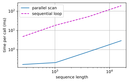
The sequential curve climbs linearly with \(T\), dominated by the cost of launching \(T\) tiny dependent steps. The scan’s curve stays well below it at every length, by roughly an order of magnitude in our runs: its handful of rounds are large batched operations that actually saturate the hardware. Thus the recurrence can be evaluated with a small number of batched operations during training. Note what the scan did not change: at inference we still update \(\mathbf{h}_t = \mathbf{a}_t \odot \mathbf{h}_{t-1} + \mathbf{b}_t\) one token at a time, in constant memory, exactly like any RNN. We make good on that claim, with a stopwatch, in Section 12.2.6.
12.2.2.3 A minGRU Language Model
Assembling Equation 12.2.1 through Equation 12.2.3 around the scan yields a drop-in replacement for the recurrent cells of Section 12.1: same (inputs, state) interface, no step-by-step loop. A carried-in state folds into the first element, since \(\mathbf{h}_1 = \mathbf{a}_1 \odot \mathbf{h}_0 + \mathbf{b}_1\).
class MinGRU(d2l.Module):
    """The minimal GRU: input-only gates and a linear state path."""
    def __init__(self, num_inputs, num_hiddens):
        super().__init__()
        self.save_hyperparameters()
        self.W_xz = nn.Linear(num_inputs, num_hiddens)
        self.W_xh = nn.Linear(num_inputs, num_hiddens)

    def forward(self, inputs, H=None):
        Z = torch.sigmoid(self.W_xz(inputs))     # (num_steps, batch, hiddens)
        H_tilde = torch.tanh(self.W_xh(inputs))
        a, b = 1 - Z, Z * H_tilde
        if H is not None:  # Fold the carried-in state into the first step
            b = torch.cat([b[:1] + a[:1] * H, b[1:]])
        outputs = associative_scan(a, b)
        return outputs, outputs[-1]
class MinGRU(nnx.Module):
"""The minimal GRU: input-only gates and a linear state path."""
def __init__(self, num_inputs, num_hiddens, rngs=None):
rngs = nnx.Rngs(0) if rngs is None else rngs
self.num_inputs, self.num_hiddens = num_inputs, num_hiddens
self.W_xz = nnx.Linear(num_inputs, num_hiddens, rngs=rngs)
self.W_xh = nnx.Linear(num_inputs, num_hiddens, rngs=rngs)
def __call__(self, inputs, H=None):
Z = jax.nn.sigmoid(self.W_xz(inputs)) # (num_steps, batch, hiddens)
H_tilde = jnp.tanh(self.W_xh(inputs))
a, b = 1 - Z, Z * H_tilde
if H is not None: # Fold the carried-in state into the first step
b = jnp.concatenate([b[:1] + a[:1] * H, b[1:]])
outputs = associative_scan(a, b)
return outputs, outputs[-1]Is stripping the GRU this aggressively survivable? We rerun the exact recipe of Section 12.1: The Time Machine under the 1,024-token BPE tokenizer, 50,000 windows of 32 tokens, embedding dimension 64, 128 hidden units, ten epochs, gradients clipped to norm 1, so the numbers are directly comparable with that section’s scoreboard.
data = d2l.TimeMachine(batch_size=1024, num_steps=32,
                       num_train=50000, num_val=5000)
data = d2l.TimeMachine(batch_size=1024, num_steps=32,
num_train=50000, num_val=5000)mingru = MinGRU(num_inputs=64, num_hiddens=128)
model = d2l.RNNLM(mingru, vocab_size=len(data.vocab), lr=4)mingru = MinGRU(num_inputs=64, num_hiddens=128)
model = d2l.RNNLM(mingru, vocab_size=len(data.vocab), lr=4)trainer = d2l.Trainer(max_epochs=10, gradient_clip_val=1, num_gpus=1)
model.board.yscale = 'log'
start = time.time()
trainer.fit(model, data)
fit_time = time.time() - start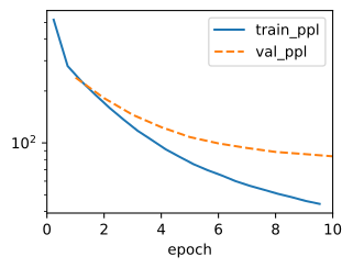
trainer = d2l.Trainer(max_epochs=10, gradient_clip_val=1, num_gpus=1)
model.board.yscale = 'log'
start = time.time()
trainer.fit(model, data)
fit_time = time.time() - start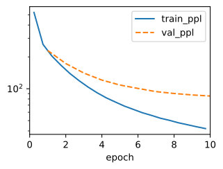
ppl = float(model.board.data['val_ppl'][-1].y)
pred = model.predict('the time traveller', 30, data.tokenizer, d2l.try_gpu())
print(f'validation perplexity {ppl:.1f}, {fit_time:.0f}s wall clock')
print(pred)
validation perplexity 83.6, 9s wall clock
the time traveller. I had a
dised. I was in the
side, and the
side, and the
side, anddef val_ppl(model):
total_loss = num_tokens = 0
for X_val, y_val in data.val_dataloader():
losses = model.loss(model(X_val), y_val, averaged=False)
total_loss += float(losses.sum())
num_tokens += losses.size
return math.exp(total_loss / num_tokens)
pred = model.predict('the time traveller', 30, data.tokenizer)
print(f'validation perplexity {val_ppl(model):.1f}, '
f'{fit_time:.0f}s wall clock')
print(pred)validation perplexity 85.3, 16s wall clock
the time traveller.
'I had
dism.
'I had
dism.
'I had
dismIn our runs the minGRU’s validation perplexity comes in a few points behind the GRU of Section 12.1.3 (low-to-mid eighties versus high seventies to low eighties under the identical recipe), despite having input-only gates and roughly a quarter of the GRU’s recurrent parameters, at \(2h(d+1)\) versus \(3h(d+h+1)\) weights. The claim here is deliberately modest: not that the minGRU is better, but that very little of the GRU’s quality is lost at this scale while the training computation becomes a parallel scan. At 32-step windows the sequential loop was never the bottleneck; the wall-clock argument is the benchmark above, whose gap keeps widening as sequences grow. What the stripped cell does give up is any dependence of the gates on the state: the decay \(\mathbf{a}_t\) is decided by the current input alone. Hold that thought; it returns as the central limitation at the end of this section.
12.2.3 State Space Models
The minGRU linearized an RNN by deletion. State space models arrive at the same destination from the opposite direction, starting from a classical object with sixty years of control-theory pedigree: the continuous-time linear dynamical system
\[ \dot{\mathbf{x}}(t) = \mathbf{A}\, \mathbf{x}(t) + \mathbf{B}\, u(t), \qquad y(t) = \mathbf{C}\, \mathbf{x}(t) + D\, u(t), \tag{12.2.5}\]
in which a scalar input signal \(u(t)\) drives a hidden state \(\mathbf{x}(t) \in \mathbb{R}^N\) through the state matrix \(\mathbf{A} \in \mathbb{R}^{N \times N}\) and input vector \(\mathbf{B} \in \mathbb{R}^{N}\), and a scalar output \(y(t)\) reads the state through \(\mathbf{C} \in \mathbb{R}^{1 \times N}\) plus a direct skip term \(D u(t)\). (For vector-valued sequences we will simply run one such system per feature channel.)
Why go continuous when our data are discrete tokens or pixels? Because Equation 12.2.5 parameterizes dynamics, a law of motion, rather than a table of per-step transition weights. The law is independent of how finely we sample it: one extra scalar, a step size \(\Delta\), converts the same \((\mathbf{A}, \mathbf{B})\) into a recurrence at any rate, so resolution becomes a knob rather than something baked into the weights. Better still, the conversion has a closed form that will hand us, for free, the gate that Section 12.1 had to engineer by hand.
12.2.3.1 Discretization: the Step Size is a Gate
To turn Equation 12.2.5 into a recurrence, hold the input constant over each sampling interval of length \(\Delta\) (a zero-order hold, ZOH) and integrate the ODE exactly across the interval. For the linear system this integral is explicit, giving the discrete recurrence
\[ \mathbf{x}_t = \bar{\mathbf{A}}\, \mathbf{x}_{t-1} + \bar{\mathbf{B}}\, u_t, \qquad y_t = \mathbf{C}\, \mathbf{x}_t + D\, u_t, \tag{12.2.6}\]
with
\[ \bar{\mathbf{A}} = \exp(\Delta \mathbf{A}), \qquad \bar{\mathbf{B}} = \left( \int_0^{\Delta} \exp(\tau \mathbf{A})\, d\tau \right) \mathbf{B}, \tag{12.2.7}\]
where \(\exp\) is the matrix exponential: the state decays under the flow for a full interval, while the held input is carried in by the flow from every instant \(\tau\) at which it entered. The integral is the definition; when \(\mathbf{A}\) is invertible it has the familiar closed form \(\bar{\mathbf{B}} = \mathbf{A}^{-1}(\exp(\Delta \mathbf{A}) - \mathbf{I})\, \mathbf{B}\), and for singular \(\mathbf{A}\) the integral still exists (at \(\mathbf{A} = \mathbf{0}\) it is simply \(\Delta \mathbf{B}\)). (A cruder alternative, the Euler step \(\bar{\mathbf{A}} \approx \mathbf{I} + \Delta \mathbf{A}\), is the subject of an exercise.) In practice \(\mathbf{A}\) is taken diagonal, \(\mathbf{A} = \mathrm{diag}(a_1, \ldots, a_N)\), which makes Equation 12.2.7 elementwise. The S4D results below provide empirical evidence for this diagonal restriction:
\[ \bar{a}_n = e^{\Delta a_n}, \qquad \bar{b}_n = \frac{e^{\Delta a_n} - 1}{a_n}\, b_n \quad (a_n \neq 0; \textrm{ the limit at } a_n = 0 \textrm{ is } \Delta b_n). \tag{12.2.8}\]
One numerical note travels with Equation 12.2.8: for small \(|\Delta a_n|\) the numerator \(e^{\Delta a_n} - 1\) cancels catastrophically in floating point, so code should call expm1, which computes \(e^x - 1\) accurately near zero. Our implementations below do.
Making \(\Delta\) a learnable parameter turns the step size into a gate.
As \(\Delta \to 0\), we get \(\bar{\mathbf{A}} \to \mathbf{I}\) and \(\bar{\mathbf{B}} \to \mathbf{0}\): the state copies itself forward and ignores the input, a frozen memory. As \(\Delta\) grows (with the real parts of the eigenvalues of \(\mathbf{A}\) negative), \(\bar{\mathbf{A}} \to \mathbf{0}\) and the state is rewritten from the current input alone. A learned \(\Delta\) is therefore an update gate in the sense of Section 12.1, interpolating between retaining the previous state and overwriting it from the current input. This correspondence follows from the rate of the continuous dynamics and provides the bridge between gated RNNs and the selective models developed next, where \(\Delta\) becomes input-dependent.
The correspondence becomes an identity, not an analogy, in one worked scalar case. Discretize the same ODE with the backward Euler rule instead of the ZOH and, for the scalar mode \(a = -1\), \(b = 1\), the update becomes \(x_t = (1 - z)\, x_{t-1} + z\, u_t\) with \(z = \Delta / (1 + \Delta)\); store the step size in log space, as we are about to, and \(z = \sigma(\log \Delta)\) is exactly a sigmoid gate. A GRU-style gated update is the backward-Euler discretization of this scalar mode, with the gate’s pre-activation playing the role of the log step size (Gu 2023). Keep the scope of the identity in view: for general matrix \(\mathbf{A}\) the backward-Euler transition \((\mathbf{I} - \Delta \mathbf{A})^{-1}\) is matrix-valued and each mode carries its own decay and tied input response, so not every discretized SSM is a GRU-style update. In this scalar case, though, the gates that Section 12.1 engineered and the step size that calculus hands us here are one object seen through two discretization rules.
ZOH and backward Euler are two entries in a standard menu. The rules differ in the transition they produce, in whether they preserve stability, and in what happens when the sampling rate changes (Table 12.2.1).
| Rule | \(\bar{\mathbf{A}}\) | \(\mathrm{Re}(a) < 0\) maps to | Accuracy | Changing \(\Delta\) |
|---|---|---|---|---|
| Zero-order hold | \(e^{\Delta \mathbf{A}}\) | \(\lvert\bar{a}\rvert < 1\), always | exact for piecewise-constant input | rediscretize; stays stable |
| Bilinear (Tustin) | \((\mathbf{I} - \tfrac{\Delta}{2}\mathbf{A})^{-1}(\mathbf{I} + \tfrac{\Delta}{2}\mathbf{A})\) | \(\lvert\bar{a}\rvert < 1\), always | second order in \(\Delta\) | rediscretize; stays stable |
| Forward Euler | \(\mathbf{I} + \Delta \mathbf{A}\) | \(\lvert 1 + \Delta a\rvert < 1\) only for small \(\Delta\) | first order in \(\Delta\) | a coarser \(\Delta\) can destabilize |
| Backward Euler | \((\mathbf{I} - \Delta \mathbf{A})^{-1}\) | \(\lvert\bar{a}\rvert < 1\), always | first order in \(\Delta\) | rediscretize; stays stable |
The choice is less about accuracy than about guarantees: every rule but forward Euler maps the stable half-plane into the stable disk for any \(\Delta\). S4 used the bilinear transform (Gu, Goel, et al. 2022); we use ZOH throughout this chapter, as Mamba does (with a further first-order simplification we meet in Section 12.3). The exercise uses forward Euler to show how its stability can fail.
Section 8.6.2.1 taught us to fear for stability; here stability is a matter of parameterization rather than luck. Store \(a_n\) as \(-e^{\theta_n}\) (or any form pinned to the left half-plane), and the discrete eigenvalues satisfy
\[ |\bar{a}_n| = e^{\Delta\, \mathrm{Re}(a_n)} < 1 \quad \textrm{whenever } \mathrm{Re}(a_n) < 0, \]
for every value of the learned parameters: the spectral radius lives inside the unit circle by construction, and no gradient update can push the recurrence into the exploding regime. One scoping remark keeps this claim exact. For a diagonal — hence normal — \(\mathbf{A}\), the eigenvalue bound controls every transient too: each coordinate shrinks at every single step. A general non-normal matrix is slipperier, since its powers can grow substantially for many steps before eigenvalue decay wins (Section 24.2.2); every \(\mathbf{A}\) this chapter trains is diagonal, so the stronger, per-step reading applies. By contrast, a vanilla RNN must learn a recurrent matrix \(\mathbf{W}_{\textrm{hh}}\) whose effective dynamics remain near \(\rho \approx 1\); gradient clipping alone does not enforce this property. Allowing complex \(a_n\) (conjugate pairs) adds rotation to the decay: each state dimension becomes a damped oscillator with a learned frequency, enriching the dynamics at no cost to stability. For everything we train below, plain negative-real \(a_n\) suffices.
Four meanings of “stable”. The word is doing several jobs in this chapter, and they are not interchangeable. Asymptotic (internal) stability: the autonomous state decays, \(\mathbf{x}_t \to \mathbf{0}\); for our diagonal systems this is exactly \(|\bar{a}_n| < 1\), and it is what “by construction” above means. BIBO stability: bounded inputs yield bounded outputs; internal stability implies it here, though the the two can differ when an unstable mode is unobservable, as the control-theory example below shows. Nonexpansive transition: a single step never increases the state norm — a stronger per-step property that returns for the delta-rule transitions of Section 12.5. Numerical stability: the floating-point computation neither loses accuracy nor overflows; a mathematically stable scan can still hit it (notes at the end of this subsection).
A last word on precision, since discretized recurrences live or die by it. Three habits cover this chapter. First, compute \(e^x - 1\) with expm1, as above. Second, respect what the scan does to rounding: it reassociates a length-\(T\) product of decays, so its output matches the sequential loop only to float tolerance, never bitwise — every check in this chapter compares against a tolerance scaled to the dtype. Third, watch long products: with all \(|\bar{a}| < 1\) a product of \(T\) decays underflows gracefully toward zero, but ratios of separately exponentiated prefix products can overflow, and the chunked forms of Section 12.4 are built from exactly those ratios; log-domain and chunk-rescaled implementations are the production answer.
12.2.3.2 Recurrence is Convolution
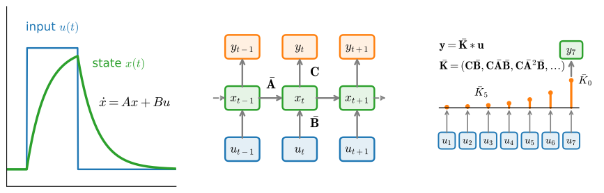
The system Equation 12.2.6 is linear and time-invariant (LTI): the same \(\bar{\mathbf{A}}, \bar{\mathbf{B}}, \mathbf{C}\) act at every step. Unroll the recurrence from \(\mathbf{x}_0 = \mathbf{0}\) and every output becomes a weighted sum of all past inputs:
\[ y_t = \sum_{k=0}^{t-1} \mathbf{C} \bar{\mathbf{A}}^{k} \bar{\mathbf{B}}\, u_{t-k} + D\, u_t = (\bar{\mathbf{K}} * \mathbf{u})_t + D\, u_t, \qquad \bar{\mathbf{K}} = (\mathbf{C}\bar{\mathbf{B}},\ \mathbf{C}\bar{\mathbf{A}}\bar{\mathbf{B}},\ \mathbf{C}\bar{\mathbf{A}}^2\bar{\mathbf{B}}, \ldots). \tag{12.2.9}\]
That is a plain causal convolution, with a kernel \(\bar{\mathbf{K}}\) as long as the sequence itself, materialized from three small matrices. The same model therefore has three equivalent views (Figure 12.2.2): a continuous ODE for analysis and parameterization, a recurrence for constant-state inference, and a convolution for parallel training. The S4 line of work trains through this convolutional view, computing \(\bar{\mathbf{K}}\) and applying it with FFTs in \(O(T \log T)\) time (Gu, Goel, et al. 2022); this method relies on time-invariance. The next section makes the dynamics input-dependent precisely to gain selectivity. The parallel scan covers both cases, so the scan is the path we implement.
For a random diagonal SSM, we compute the same outputs three ways: with the sequential recurrence, the parallel scan, and convolution with the materialized kernel from Equation 12.2.9 (we drop the \(D\) skip here, since all three views share it verbatim).
num_states, num_steps, delta = 8, 64, 0.1
a = -torch.arange(1., num_states + 1)               # Re(a) < 0
b, c = torch.ones(num_states), torch.randn(num_states)
a_bar = torch.exp(delta * a)                        # Zero-order hold
b_bar = torch.expm1(delta * a) / a * b              # expm1: accurate e^x - 1
u = torch.randn(num_steps)

x, ys = torch.zeros(num_states), []                 # (i) recurrence
for t in range(num_steps):
    x = a_bar * x + b_bar * u[t]
    ys.append(torch.dot(c, x))
y_loop = torch.stack(ys)

xs = associative_scan(a_bar.tile(num_steps, 1),     # (ii) parallel scan
                      b_bar * u[:, None])
y_scan = xs @ c

k = torch.arange(num_steps)[:, None]                # (iii) convolution
kernel = (c * b_bar * a_bar ** k).sum(-1)
y_conv = torch.tensor(np.convolve(u, kernel)[:num_steps])

print(f'scan vs loop: {float((y_scan - y_loop).abs().max()):.2e}, '
      f'conv vs loop: {float((y_conv - y_loop).abs().max()):.2e}')
scan vs loop: 2.38e-07, conv vs loop: 2.38e-07num_states, num_steps, delta = 8, 64, 0.1
a = -jnp.arange(1., num_states + 1) # Re(a) < 0
b, c = jnp.ones(num_states), jax.random.normal(d2l.get_key(), (num_states,))
a_bar = jnp.exp(delta * a) # Zero-order hold
b_bar = jnp.expm1(delta * a) / a * b # expm1: accurate e^x - 1
u = jax.random.normal(d2l.get_key(), (num_steps,))
def step(x, u_t): # (i) recurrence
x = a_bar * x + b_bar * u_t
return x, jnp.dot(c, x)
_, y_loop = jax.lax.scan(step, jnp.zeros(num_states), u)
xs = associative_scan(jnp.tile(a_bar, (num_steps, 1)),
b_bar * u[:, None]) # (ii) parallel scan
y_scan = xs @ c
k = jnp.arange(num_steps)[:, None] # (iii) convolution
kernel = (c * b_bar * a_bar ** k).sum(-1)
y_conv = jnp.array(np.convolve(u, kernel)[:num_steps])
print(f'scan vs loop: {float(jnp.abs(y_scan - y_loop).max()):.2e}, '
f'conv vs loop: {float(jnp.abs(y_conv - y_loop).max()):.2e}')scan vs loop: 8.94e-08, conv vs loop: 1.19e-07The three views agree to floating-point precision. Each view supports a different operation, and linearity makes it possible to switch among them.
12.2.3.3 Interpretation from Control Theory
State space models were not invented for deep learning: they are the core formalism of 1960s control theory. Four concepts clarify the models used in this chapter. All four show up in the smallest interesting example, a two-state diagonal system
\[ \dot{\mathbf{x}}(t) = \begin{pmatrix} -1 & 0 \\ 0 & -2 \end{pmatrix} \mathbf{x}(t) + \mathbf{B}\, u(t), \qquad y(t) = \mathbf{C}\, \mathbf{x}(t). \]
Controllability and observability. With \(\mathbf{B} = (1, 0)^\top\) the input never touches the second state: that mode is uncontrollable, and no input signal can move it off its decay. With \(\mathbf{C} = (1, 0)\) the output never sees it: the mode is unobservable. Either way, the two-state system behaves at its terminals exactly like a one-state system. State size is therefore an upper bound on dynamical richness rather than a measurement of it: \(N\) counts coordinates, not the amount of memory the model uses.
Transfer function and poles. Solved in the frequency domain, the LTI system is multiplication by the transfer function \(H(s) = \mathbf{C}(s\mathbf{I} - \mathbf{A})^{-1}\mathbf{B}\), a rational function whose poles are a subset of the eigenvalues of \(\mathbf{A}\). For the example with \(\mathbf{B} = (1, 0)^\top\) and \(\mathbf{C} = (1, 1)\), \(H(s) = 1/(s+1)\): one pole, not two, because the unreachable mode cancels. The impulse response — our convolution kernel Equation 12.2.9 — is the same object in the time domain; the kernel view above is control theory’s oldest view, rediscovered.
Internal versus BIBO stability. The cancellation is also where the two stability notions of the box above part ways: a system can be BIBO stable, with bounded inputs producing bounded outputs, while an unstable mode grows unseen because it is hidden from the output. The stronger certificate is internal stability, every mode decaying, and that is what our left-half-plane parameterization provides.
Similarity and non-identifiability. Change state coordinates by any invertible \(\mathbf{T}\), sending \((\mathbf{A}, \mathbf{B}, \mathbf{C})\) to \((\mathbf{T}\mathbf{A}\mathbf{T}^{-1}, \mathbf{T}\mathbf{B}, \mathbf{C}\mathbf{T}^{-1})\), and the input–output map is unchanged. The state is a coordinate system, not a canonical object. That freedom is why restricting \(\mathbf{A}\) to diagonal form (as S4D will) is less of a sacrifice than it looks, and why two different-looking recurrences can compute one function — a theme that returns as the state-space duality of Section 12.4. For the classical theory at full strength, see Åström and Murray (2021) .
The term has a different scope in statistics and signal processing. In statistics and signal processing a “state space model” is usually stochastic: process noise drives the state, observation noise corrupts the output, and the computational problem is inference — recovering a posterior over the latent trajectory, by the Kalman filter (Kalman 1960) in the linear-Gaussian case and by particle methods beyond it, with system identification as the matching learning problem. The SSMs of this chapter share the state equation but not the problem: they are deterministic feature extractors trained by backpropagation, with no noise model and no posterior. The shared name records lineage, not equivalence.
12.2.4 HiPPO Memory Initialization
One question remains before we can call this a principled design: what should \(\mathbf{A}\) be? Stability constrains its eigenvalues to the left half-plane but otherwise leaves \(N^2\) (or \(N\) diagonal) numbers to choose, and early attempts to train SSMs from random initializations performed poorly. The question has a crisp mathematical form. The state \(\mathbf{x}(t)\) is a fixed budget of \(N\) numbers summarizing the input seen so far; which \(N\) numbers lose the least?
HiPPO (high-order polynomial projection operators) provides one answer (Gu et al. 2020). Fix a measure over the past, say uniform weight on everything seen so far, and ask that \(\mathbf{x}(t)\) hold the \(N\) coefficients of the best orthogonal polynomial approximation (of degree less than \(N\)) of the input’s history under that measure, the same least-squares projection that underlies Fourier and Legendre series. A central HiPPO result is that this optimal compression can be maintained online: as new input arrives, the optimal coefficients evolve according to a linear, time-varying ODE,
\[ \dot{\mathbf{x}}(t) = \frac{1}{t} \left( \mathbf{A}\, \mathbf{x}(t) + \mathbf{B}\, u(t) \right), \tag{12.2.10}\]
with a specific, input-independent matrix. For the uniform (“scaled Legendre”, LegS) measure it is
\[ A_{nk} = -\begin{cases} \sqrt{(2n+1)(2k+1)} & \textrm{if } n > k, \\ n + 1 & \textrm{if } n = k, \\ 0 & \textrm{if } n < k, \end{cases} \qquad B_n = \sqrt{2n + 1}, \tag{12.2.11}\]
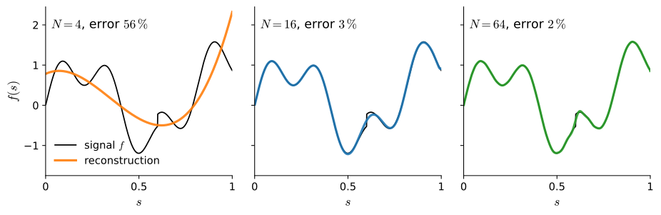
for \(n, k = 0, \ldots, N-1\). We state the matrix and cite the derivation. The factor \(1/t\) makes Equation 12.2.10 not an instance of the LTI system Equation 12.2.5. The measure spreads uniform weight over all of \([0, t]\), so by time \(t\) each new instant is only a \(1/t\) fraction of the history it joins, and the dynamics must slow down accordingly: discretized at unit steps the update is \(\mathbf{x}_k = (\mathbf{I} + \mathbf{A}/k)\, \mathbf{x}_{k-1} + (\mathbf{B}/k)\, u_k\), a recurrence whose effective step size decays like \(1/k\) rather than holding constant. The system has no timescale \(\Delta\) to tune because rescaling time maps its trajectories onto themselves. The consequence of the theorem appears in Figure 12.2.3, whose generator integrates exactly this time-varying system: a signal is compressed online into a LegS state of size \(N\) and then reconstructed from the state alone at the final time. With \(N = 64\) numbers, a thousand-step history is recovered almost perfectly, smoothing only the sharpest transients. A fixed-size state provably can carry a long past, provided its dynamics are chosen for the job.
12.2.4.1 From HiPPO to S4 to S4D
The path from this theorem to the layer we implement passes through three different objects, and it pays to keep them distinct.
The online LegS projection is the time-varying system Equation 12.2.10. It, and only it, carries the optimality theorem: run those dynamics and the state is, at every moment, the best degree-\(N\) polynomial summary of the entire past under the uniform measure.
S4 is an LTI model initialized at the HiPPO matrix. S4 (Gu, Goel, et al. 2022) freezes Equation 12.2.11 into the time-invariant system Equation 12.2.5, adds a learnable step size per channel, and trains the resulting parameters by gradient descent. The optimality theorem does not transfer — a time-invariant system maintains no uniform-measure projection; tracking one is precisely what the \(1/t\) was for — but the HiPPO matrix provides an effective initialization, giving the state a spread of decay timescales and long-memory structure that random matrices lack. Speed came from structure: the HiPPO matrix is normal plus low-rank (NPLR), so it is unitarily similar to a diagonal-plus-low-rank (DPLR) matrix with complex-conjugate modes, and with that form the convolution kernel Equation 12.2.9 reduces to Cauchy-kernel evaluations computable in near-linear time — machinery we cite rather than rebuild. On the Long Range Arena benchmark (Tay et al. 2021), S4 outperformed the compared transformers on tasks with dependencies over 16,000 steps.
S4D is the diagonal approximation. Drop the low-rank correction and keep a diagonal state matrix, collapsing the machinery to the elementwise formulas Equation 12.2.8. Gu, Gupta, et al. (2022) supply the evidence that this step is safe: suitably initialized diagonal systems approximate S4’s kernel as the state grows and match its accuracy across the Long Range Arena in practice. The simplest of their initializations is the one we implement below, real \(a_n = -(n + 1)\), the diagonal of Equation 12.2.11. Be clear about what that inherits and what it does not: it is a multiscale initialization, a bank of decay rates from slow to fast, not the optimal Legendre projection — the theorem stays behind with the time-varying system, and the case for the diagonal model is the S4D paper’s empirical one. Finally, S5 (Smith et al. 2023) replaced the per-channel FFTs with one multi-input state space layer evaluated by the parallel scan, the same computational pattern we built above. Our implementation sits deliberately at the intersection: S4D’s diagonal parameterization, S5’s scan.
12.2.5 S4D in Practice
Time to assemble a working network. The S4D layer below runs one independent scalar SSM per feature channel, each with \(N\) internal states: its parameters are the diagonal \(\mathbf{a}\) (stored as \(-e^{\log \textrm{magnitude}}\) to pin eigenvalues to the left half-plane, initialized to \(-(n+1)\)), a per-channel learnable step size \(\Delta\) (stored as \(\log \Delta\), initialized log-uniformly between \(10^{-3}\) and \(10^{-1}\), so different channels start as gates of very different speeds), the read-out \(\mathbf{C}\), and the skip \(D\); following S4D we fix \(\mathbf{B} = \mathbf{1}\) and let \(\mathbf{C}\) absorb its scale. The forward pass is three lines of ZOH followed by the scan from Section 12.2.2; since the dynamics are time-invariant, the decay coefficients are the same at every position, and broadcasting (a singleton batch axis for a) spares us materializing them per element. We save the layer, and the block that follows, in the d2l library: the next section builds directly on both.
class S4D(nn.Module):
    """A diagonal state space layer: one SSM per feature channel."""
    def __init__(self, num_hiddens, num_states=4, dt_min=0.001, dt_max=0.1):
        super().__init__()
        H, N = num_hiddens, num_states
        self.log_a = nn.Parameter(
            torch.log(torch.arange(1., N + 1)).repeat(H, 1))
        self.log_dt = nn.Parameter(
            torch.rand(H, 1) * math.log(dt_max / dt_min) + math.log(dt_min))
        self.C = nn.Parameter(torch.randn(H, N) / math.sqrt(N))
        self.D = nn.Parameter(torch.ones(H))

    def forward(self, u):                    # (num_steps, batch, num_hiddens)
        a = -torch.exp(self.log_a)                    # (H, N), Re(a) < 0
        da = torch.exp(self.log_dt) * a
        a_bar = torch.exp(da)
        b_bar = torch.expm1(da) / a                   # ZOH with B = 1
        a_elems = a_bar.expand(u.shape[0], 1, -1, -1) # Same at every step
        b_elems = b_bar * u.unsqueeze(-1)             # (T, batch, H, N)
        x = associative_scan(a_elems, b_elems)
        return (x * self.C).sum(-1) + self.D * u
class S4D(nnx.Module):
"""A diagonal state space layer: one SSM per feature channel."""
def __init__(self, num_hiddens, num_states=4, dt_min=0.001, dt_max=0.1,
rngs=None):
rngs = nnx.Rngs(0) if rngs is None else rngs
H, N = num_hiddens, num_states
self.log_a = nnx.Param(jnp.tile(jnp.log(jnp.arange(1., N + 1)),
(H, 1)))
self.log_dt = nnx.Param(
rngs.params.uniform((H, 1)) * math.log(dt_max / dt_min)
+ math.log(dt_min))
self.C = nnx.Param(rngs.params.normal((H, N)) / math.sqrt(N))
self.D = nnx.Param(jnp.ones(H))
def __call__(self, u): # (num_steps, batch, num_hiddens)
a = -jnp.exp(self.log_a[...]) # (H, N), Re(a) < 0
da = jnp.exp(self.log_dt[...]) * a
a_bar = jnp.exp(da)
b_bar = jnp.expm1(da) / a # ZOH with B = 1
a_elems = jnp.broadcast_to( # Same at every step
a_bar[None, None], (u.shape[0], 1, *a_bar.shape))
b_elems = b_bar * u[..., None] # (T, batch, H, N)
x = associative_scan(a_elems, b_elems)
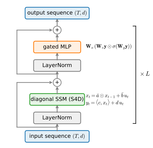
return (x * self.C).sum(-1) + self.D * uA single S4D layer mixes information across time but never across channels (each channel owns a private SSM), and it is linear. Both gaps are closed the modern way, by wrapping the layer in a residual block with normalization and a gated MLP (Figure 12.2.4): the MLP mixes channels and supplies the nonlinearity that the state path gave up, and the gate is one more echo of Section 12.1. Stacking \(L\) such blocks yields the standard deep SSM of the S4/S4D/S5 papers.
class S4DBlock(nn.Module):
    def __init__(self, num_hiddens, num_states):
        super().__init__()
        self.ln1 = nn.LayerNorm(num_hiddens)
        self.ssm = S4D(num_hiddens, num_states)
        self.ln2 = nn.LayerNorm(num_hiddens)
        self.W_v = nn.Linear(num_hiddens, 2 * num_hiddens)
        self.W_g = nn.Linear(num_hiddens, 2 * num_hiddens)
        self.W_o = nn.Linear(2 * num_hiddens, num_hiddens)

    def forward(self, X):
        X = X + self.ssm(self.ln1(X))
        Y = self.ln2(X)
        return X + self.W_o(self.W_v(Y) * torch.sigmoid(self.W_g(Y)))
class S4DBlock(nnx.Module):
def __init__(self, num_hiddens, num_states, rngs=None):
rngs = nnx.Rngs(0) if rngs is None else rngs
self.ln1 = nnx.LayerNorm(num_hiddens, rngs=rngs)
self.ssm = S4D(num_hiddens, num_states, rngs=rngs)
self.ln2 = nnx.LayerNorm(num_hiddens, rngs=rngs)
self.W_v = nnx.Linear(num_hiddens, 2 * num_hiddens, rngs=rngs)
self.W_g = nnx.Linear(num_hiddens, 2 * num_hiddens, rngs=rngs)
self.W_o = nnx.Linear(2 * num_hiddens, num_hiddens, rngs=rngs)
def __call__(self, X):
X = X + self.ssm(self.ln1(X))
Y = self.ln2(X)
return X + self.W_o(self.W_v(Y) * jax.nn.sigmoid(self.W_g(Y)))12.2.5.1 Sequential Image Classification
Where should a long-memory architecture prove itself? A classic stress test is sequential image classification: feed a model the Fashion-MNIST images of Section 3.2 one pixel at a time, as a plain sequence of 784 scalars, and predict the class. No spatial structure is given: any relation between pixel 3 and pixel 787 must travel through the sequence model. How it is allowed to travel is decided by the readout, and the choice changes what the experiment measures. Mean-pooling all 784 per-step outputs is the standard benchmark form of the task: every pixel contributes through its own output, so the score measures how well the encoder mixes information across the sequence, not whether anything survives to the end. Reading only the final step’s features is the sterner retention diagnostic: whatever the model uses must still be present in the state after hundreds of updates. The classifier below embeds each pixel, runs an encoder over the sequence, and supports both readouts; it accepts any encoder with our (num_steps, batch, features) calling convention, which lets us swap an S4D stack against an LSTM without touching anything else. We train with Adam (Chapter 9), whose per-parameter step sizes suit a model that mixes log-decays with ordinary linear weights; plain SGD handles the SSM’s exponentials awkwardly.
class SeqClassifier(d2l.Classifier):
    """Classify a sequence: encoder, then mean or final-step readout."""
    def __init__(self, encoder, num_hiddens, pool='mean', lr=3e-3):
        super().__init__()
        self.save_hyperparameters()
        self.emb = nn.Linear(1, num_hiddens)
        self.head = nn.LazyLinear(10)

    def forward(self, X):
        X = X.reshape(X.shape[0], -1, 1).movedim(1, 0)  # Pixel sequence
        Y = self.encoder(self.emb(X))
        Y = Y[0] if isinstance(Y, tuple) else Y         # RNNs return a state
        return self.head(Y.mean(dim=0) if self.pool == 'mean' else Y[-1])

    def configure_optimizers(self):
        return torch.optim.Adam(self.parameters(), lr=self.lr)
class SeqClassifier(d2l.Classifier):
"""Classify a sequence: encoder, then mean or final-step readout."""
def __init__(self, encoder, num_hiddens, num_features=None, pool='mean',
lr=3e-3, rngs=None):
super().__init__()
self.save_hyperparameters(ignore=['encoder', 'rngs'])
rngs = nnx.Rngs(1) if rngs is None else rngs
num_features = num_hiddens if num_features is None else num_features
self.encoder = encoder
self.emb = nnx.Linear(1, num_hiddens, rngs=rngs)
self.head = nnx.Linear(num_features, 10, rngs=rngs)
def forward(self, X):
X = X.reshape(X.shape[0], -1, 1).transpose(1, 0, 2) # Pixel sequence
Y = self.encoder(self.emb(X))
Y = Y[0] if isinstance(Y, tuple) else Y # RNNs return a state
return self.head(Y.mean(axis=0) if self.pool == 'mean' else Y[-1])
def configure_optimizers(self):
return optax.adam(self.lr)Our S4D model stacks two blocks of width 48 with \(N = 4\) states per channel; the baseline is the LSTM of Section 12.1 sized to the same parameter count (48-dimensional pixel embeddings, 64 hidden units, roughly 30,000 parameters each), trained under the benchmark mean-pool readout. Ten epochs each, identical data pipeline, identical head, and gradients clipped to norm 1 for both models: at 784 steps the LSTM otherwise destabilizes mid-training, its loss spiking exactly as Section 8.6.2.1 would predict, while the S4D, whose recurrence cannot leave the unit circle, reaches the same accuracy with or without clipping.
data = d2l.FashionMNIST(batch_size=128)
results = {}

def train_and_report(name, model, epochs=10):
    trainer = d2l.Trainer(max_epochs=epochs, gradient_clip_val=1, num_gpus=1)
    start = time.time()
    trainer.fit(model, data)
    params = sum(p.numel() for p in model.parameters() if p.requires_grad)
    results[name] = (params, float(model.board.data['val_acc'][-1].y),
                     (time.time() - start) / epochs)

s4d = SeqClassifier(nn.Sequential(*[S4DBlock(48, 4) for _ in range(2)]),
                    num_hiddens=48)
train_and_report('S4D', s4d)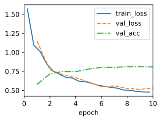
data = d2l.FashionMNIST(batch_size=128)
results = {}

def train_and_report(name, model, epochs=10):
    trainer = d2l.Trainer(max_epochs=epochs, gradient_clip_val=1, num_gpus=1)
    start = time.time()
    trainer.fit(model, data)
    params = sum(p.size for p in
                 jax.tree.leaves(nnx.state(model, nnx.Param)))
    results[name] = (params, float(model.board.data['val_acc'][-1].y),
                     (time.time() - start) / epochs)

s4d = SeqClassifier(nnx.Sequential(*[S4DBlock(48, 4) for _ in range(2)]),
                    num_hiddens=48)
train_and_report('S4D', s4d)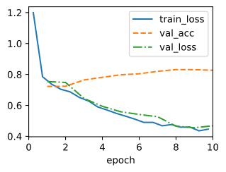
The retention diagnostic is the same mixer read only at the final step, one more training run.
s4d_final = SeqClassifier(
    nn.Sequential(*[S4DBlock(48, 4) for _ in range(2)]),
    num_hiddens=48, pool='last')
train_and_report('S4D (final)', s4d_final)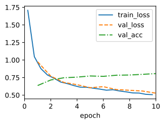
s4d_final = SeqClassifier(
    nnx.Sequential(*[S4DBlock(48, 4) for _ in range(2)]),
    num_hiddens=48, pool='last')
train_and_report('S4D (final)', s4d_final)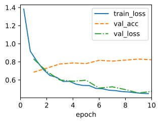
if tab.selected('pytorch'):
    lstm = SeqClassifier(d2l.LSTM(num_inputs=48, num_hiddens=64),
                         num_hiddens=48)
if tab.selected('jax'):
    lstm = SeqClassifier(d2l.LSTM(num_inputs=48, num_hiddens=64),
                         num_hiddens=48, num_features=64)
train_and_report('LSTM', lstm)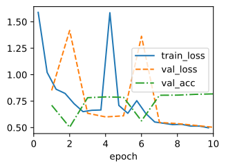
if tab.selected('pytorch'):
    lstm = SeqClassifier(d2l.LSTM(num_inputs=48, num_hiddens=64),
                         num_hiddens=48)
if tab.selected('jax'):
    lstm = SeqClassifier(d2l.LSTM(num_inputs=48, num_hiddens=64),
                         num_hiddens=48, num_features=64)
train_and_report('LSTM', lstm)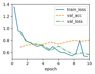
print(f'{"model":>12} {"params":>8} {"val acc":>8} {"s/epoch":>8}')
for name, (params, acc, secs) in results.items():
    print(f'{name:>12} {params:>8,} {acc:>8.3f} {secs:>8.1f}')
model params val acc s/epoch
S4D 30,058 0.808 47.6
S4D (final) 30,058 0.806 36.9
LSTM 29,930 0.819 4.0print(f'{"model":>12} {"params":>8} {"val acc":>8} {"s/epoch":>8}')
for name, (params, acc, secs) in results.items():
print(f'{name:>12} {params:>8,} {acc:>8.3f} {secs:>8.1f}') model params val acc s/epoch
S4D 30,058 0.827 6.1
S4D (final) 30,058 0.823 5.8
LSTM 29,674 0.805 48.6The table supports two separate comparisons. On the mean-pool benchmark, the S4D lands in the low-to-mid eighties in both frameworks and every rerun, clipped or unclipped. The final-state run answers the retention question the mean pool cannot: reading nothing but the state after 784 updates costs the S4D little to nothing in our runs — the two readouts finish within run-to-run noise of each other, at most a few points apart and sometimes nearly tied — so what the classifier uses genuinely survives to the end of the sequence rather than being recovered from early outputs. The LSTM baseline is more variable: across repeated runs (with and without clipping, at nearby learning rates) its final accuracy has ranged from roughly 60 to 84 percent, and the result depends strongly on initialization. Plain uniform recurrent weights (PyTorch’s default) produce less reliable long-range retention than orthogonal recurrent weights (Flax’s default). A forget-gate bias of 1, discussed in Section 12.1, further improves this initialization. The initialization explains an important part of the measured contrast. At initialization, the S4D’s channels already implement a bank of exponential memories with time constants spanning more than two orders of magnitude (what the log-uniform \(\Delta\) init provides), so pixel-to-pixel structure hundreds of steps apart is visible to the model from the first gradient step in either framework. The LSTM requires an appropriate initialization to retain state reliably in this experiment. What the SSM parameterization provides — stability by construction and a multiscale initialization — is that memory by design, robustly, rather than by folklore. The table also gives wall-clock per epoch, which depends on what each framework fuses: against PyTorch’s cuDNN-fused LSTM our teaching-grade scan pays its log-factor overhead, while in JAX, where both models run compiled scans, the parallel scan is several times faster than the sequential LSTM; production SSM kernels close the remaining gap the same way cuDNN once did for the LSTM. On the Long Range Arena (Tay et al. 2021), with sequences up to 16,000 steps, this architecture family was the first to solve tasks on which both RNNs and transformers had failed. This result motivated subsequent work on state space sequence models.
12.2.6 Inference, One Token at a Time
The scan provides parallel training. At inference, the same model can run recurrently with a fixed-size state and constant work per token; the next experiment verifies this second property. Equation Equation 12.2.6 is also the inference update. Given the last state \(\mathbf{x}_{t-1}\) and one new input \(u_t\),
\[ \mathbf{x}_t = \bar{\mathbf{A}}\, \mathbf{x}_{t-1} + \bar{\mathbf{B}}\, u_t, \qquad y_t = \mathbf{C}\, \mathbf{x}_t + D\, u_t, \]
and the state is all the model ever needs to remember: for our S4D layer, one \(N\)-vector per channel, an \((H, N)\) block of numbers per layer. The step method below advances that block by one token; the matching method on S4DBlock threads the state through the layer while the gated MLP, which acts position-wise, needs no state at all. Both go into the d2l library next to their classes.
@d2l.add_to_class(S4D)
def step(self, u, x=None):
    """Advance one token: u is (batch, H); x is the (batch, H, N) state."""
    a = -torch.exp(self.log_a)
    da = torch.exp(self.log_dt) * a
    a_bar = torch.exp(da)                             # Same ZOH as forward
    b_bar = torch.expm1(da) / a
    if x is None:
        x = u.new_zeros(*u.shape, a_bar.shape[-1])
    x = a_bar * x + b_bar * u.unsqueeze(-1)           # One recurrence step
    return (x * self.C).sum(-1) + self.D * u, x

@d2l.add_to_class(S4DBlock)
def step(self, X, x=None):
    """Advance the block one token; only the SSM carries state."""
    y, x = self.ssm.step(self.ln1(X), x)
    X = X + y
    Y = self.ln2(X)
return X + self.W_o(self.W_v(Y) * torch.sigmoid(self.W_g(Y))), x@d2l.add_to_class(S4D)
def step(self, u, x=None):
"""Advance one token: u is (batch, H); x is the (batch, H, N) state."""
a = -jnp.exp(self.log_a[...])
da = jnp.exp(self.log_dt[...]) * a
a_bar = jnp.exp(da) # Same ZOH as forward
b_bar = jnp.expm1(da) / a
if x is None:
x = jnp.zeros((*u.shape, a_bar.shape[-1]))
x = a_bar * x + b_bar * u[..., None] # One recurrence step
return (x * self.C).sum(-1) + self.D * u, x
@d2l.add_to_class(S4DBlock)
def step(self, X, x=None):
"""Advance the block one token; only the SSM carries state."""
y, x = self.ssm.step(self.ln1(X), x)
X = X + y
Y = self.ln2(X)
return X + self.W_o(self.W_v(Y) * jax.nn.sigmoid(self.W_g(Y))), xA claim of equivalence should be checked on a model whose answers we care about, so we replay validation images through the trained classifier’s encoder both ways: all 784 pixels at once through the scan, then one pixel at a time through step, carrying one state per block. The two schedules perform the same arithmetic in different association orders, so they can differ only by float32 rounding, and over 784 steps of trained, near-unit decays that rounding accumulates; the comparison must therefore be relative to the activation scale. The assertion is a regression guard as much as a demonstration: a genuine mismatch between forward and step shows up at relative errors near one, five orders of magnitude above this gate.
X_val = next(iter(data.val_dataloader()))[0][:64].to(d2l.try_gpu())
with torch.no_grad():
    seq = s4d.emb(X_val.reshape(X_val.shape[0], -1, 1).movedim(1, 0))
    y_scan = s4d.encoder(seq)                    # All 784 steps at once
    states, ys = [None] * len(s4d.encoder), []
    for t in range(seq.shape[0]):                # One pixel at a time
        X, new_states = seq[t], []
        for blk, x in zip(s4d.encoder, states):
            X, x = blk.step(X, x)
            new_states.append(x)
        states, ys = new_states, ys + [X]
err = float((torch.stack(ys) - y_scan).abs().max())
scale = float(y_scan.abs().max())
print(f'stepped vs scanned: deviation {err:.2e} '
      f'on activations of scale {scale:.0f}: relative {err / scale:.2e}')
assert err < 1e-3 * scale
stepped vs scanned: deviation 4.41e-04 on activations of scale 71: relative 6.21e-06X_val = jnp.asarray(next(iter(data.val_dataloader()))[0][:64])
seq = s4d.emb(X_val.reshape(X_val.shape[0], -1, 1).transpose(1, 0, 2))
# GPU matmuls default to TF32; run both schedules in full fp32 so the
# comparison isolates the reassociation error
with jax.default_matmul_precision('float32'):
y_scan = s4d.encoder(seq) # All 784 steps at once
states, ys = [None] * len(s4d.encoder.layers), []
for t in range(seq.shape[0]): # One pixel at a time
X, new_states = seq[t], []
for blk, x in zip(s4d.encoder.layers, states):
X, x = blk.step(X, x)
new_states.append(x)
states, ys = new_states, ys + [X]
err = float(jnp.abs(jnp.stack(ys) - y_scan).max())
scale = float(jnp.abs(y_scan).max())
print(f'stepped vs scanned: deviation {err:.2e} '
f'on activations of scale {scale:.0f}: relative {err / scale:.2e}')
assert err < 1e-3 * scalestepped vs scanned: deviation 1.67e-03 on activations of scale 79: relative 2.12e-05We next measure inference cost on a batch of 32 sequences arriving one token at a time, and consider the cost of absorbing the next token once \(P\) tokens have already passed. Without a carried state we would do what our training path does: re-run the scan over all \(P + 1\) positions, paying for the entire history again. With the state, the past is already summarized and one step suffices. We time both as the prefix grows.
def one_step(X, states):
    with torch.no_grad():
        for i, blk in enumerate(s4d.encoder):
            X, states[i] = blk.step(X, states[i])
    return X

def rerun(seq):
    with torch.no_grad():
        return s4d.encoder(seq)

lengths, times = [256, 1024, 4096, 16384], [[], []]
states = [None] * len(s4d.encoder)
for P in lengths:
    seq = torch.randn(P, 32, 48, device=device)
    one_step(seq[-1], states)                    # Materialize the state
    times[0].append(wall_clock(one_step, seq[-1], states) * 1e3)
    times[1].append(wall_clock(rerun, seq) * 1e3)
d2l.plot(lengths, times, 'prefix length', 'ms per new token',
         legend=['recurrent step', 're-run the prefix'],
         xscale='log', yscale='log', figsize=(5, 3))
print(f'carried state: {sum(4 * x.numel() for x in states) // 32} '
      f'bytes per sequence, at every prefix length')
carried state: 1536 bytes per sequence, at every prefix length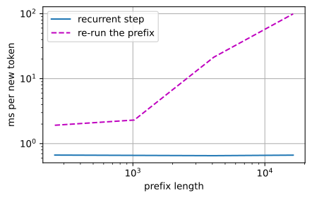
def one_step(model, X, states):
    for blk, x in zip(model.layers, states):
        X, x = blk.step(X, x)
    return X

step_fn = nnx.jit(one_step)
rerun_fn = nnx.jit(lambda model, seq: model(seq))

lengths, times = [256, 1024, 4096, 16384], [[], []]
states = [jnp.zeros((32, 48, 4)) for _ in s4d.encoder.layers]
X1 = jnp.zeros((32, 48))
for P in lengths:
    seq = jax.random.normal(jax.random.key(P), (P, 32, 48))
    times[0].append(wall_clock(step_fn, s4d.encoder, X1, states) * 1e3)
    times[1].append(wall_clock(rerun_fn, s4d.encoder, seq) * 1e3)
d2l.plot(lengths, times, 'prefix length', 'ms per new token',
         legend=['recurrent step', 're-run the prefix'],
         xscale='log', yscale='log', figsize=(5, 3))
print(f'carried state: {sum(4 * x.size for x in states) // 32} '
      f'bytes per sequence, at every prefix length')
carried state: 1536 bytes per sequence, at every prefix length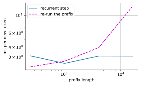
The two curves have the predicted shapes. Re-running the prefix costs more the longer the history, linearly once the sequence is long enough for real work to dominate per-call overhead; the recurrent step costs the same at every prefix length. How wide the gap has grown by our longest prefix depends on the framework’s per-call overhead (severalfold to two orders of magnitude in our runs), and it keeps widening for as long as the prefix, and the memory holding it, keep growing. At this toy width the absolute times are launch-overhead-bound, so read the shapes, not the milliseconds.
The printed number gives the corresponding memory comparison. A transformer generating with a KV cache also avoids re-running its prefix, but it does so by storing the past: its cache grows linearly with context, at a rate we measured in Section 11.3 (tens of kibibytes per token for even a small model), and serving budgets are set by that growth. The recurrent model’s entire memory of an arbitrarily long history is the \((H, N)\) state per layer printed above, about a kibibyte here, the same at token 100 as at token 100,000. This constant-memory inference motivates the use of recurrent layers in language models. Linear attention obtains this property by replacing softmax attention, as described in Section 10.5. What the fixed-size state cannot retain, and when that limitation matters, is a question this chapter returns to once the selective models are on the table.
12.2.7 Summary
Recurrence buys constant-memory inference but serializes training; this section removed the serialization by making the state update linear. The minGRU shows the deletion route: gates computed from the input alone turn the GRU into an elementwise affine recurrence \(\mathbf{h}_t = \mathbf{a}_t \odot \mathbf{h}_{t-1} + \mathbf{b}_t\), which an associative combine evaluates in \(O(\log T)\) parallel rounds, at language-modeling quality on par with the GRU. State space models reach the same recurrence from first principles: discretizing continuous linear dynamics yields the ZOH formulas, in which the learnable step size \(\Delta\) is an update gate and stability holds by construction, with eigenvalues pinned inside the unit circle by parameterization rather than by clipping (Section 8.6.2.1). Time-invariance makes the same model a recurrence, a convolution, and an ODE at once. HiPPO supplies dynamics under which a fixed-size state is a provably good compression of the whole past — a time-varying system whose matrix, frozen, initializes the LTI S4 family, with the diagonal S4D as the empirically vindicated simplification we implement. Assembled into residual blocks, the S4D trains reliably on 784-step sequential image classification where a plainly initialized, parameter-matched LSTM succeeds only on a lucky draw, and it holds its accuracy to within a few points when read from the final state alone, the retention diagnostic. Finally we ran the trained model the other way, one token at a time: stepping agrees with the scan to floating-point accuracy, costs the same at any prefix length, and carries a state a few hundred bytes per layer where a transformer’s KV cache grows with the length of the context (Section 11.3).
The state update here remains linear and time-invariant: the kernel \(\bar{\mathbf{K}}\) is fixed before the model ever sees the input, and with it the decision of what to remember. An S4D layer cannot read a token and decide that this one matters while its neighbor is noise: its gates, unlike the LSTM’s, do not look at the data as it flows past, so the state-update operator is in this precise sense content-blind. The qualifier matters: the blocks around each SSM are input-dependent, and a deep stack can modulate between layers what it cannot modulate within the state update — which is why such models earn partial credit, though not success, on the selectivity task of the next section. That section cures the limitation at the operator level while keeping the scan.
Experimental scope. The scan-vs-loop and step-vs-rerun benchmarks establish shapes (logarithmic against linear, flat against growing), measured with teaching-grade kernels on one GPU; they are not production throughput numbers. The equivalence checks (scan against loop, stepping against scanning) are identities up to float rounding, the strongest claims here. The classifier is one seeded run per framework per readout: it shows that the multiscale initialization trains reliably where the plainly initialized LSTM is at the mercy of its draw, not a general architecture ranking.
12.2.8 Exercises
Closure under composition. Function composition is always associative, so what a parallel scan needs from a recurrence is closure: the composite of any run of steps must be described by as many numbers as a single step, so that every combine costs the same.
- Generalize Equation 12.2.4 to the dense affine recurrence \(\mathbf{h}_t = \mathbf{A}_t \mathbf{h}_{t-1} + \mathbf{b}_t\) with \(\mathbf{A}_t \in \mathbb{R}^{N \times N}\), keeping the factors of each matrix product in the right order. Count the multiply-adds of one combine and of one sequential step. The doubling scan of Figure 12.2.1 performs about \(T \log_2 T\) combines; compare its total work with that of the sequential loop at \(T = 4096\) and \(N = 64\). What does the comparison say about the diagonal restriction of Section 12.2.3.1?
- For the scalar nonlinear step \(h \mapsto \tanh(w_t h + c_t)\), show that the composite of two steps with \(w_1, w_2 \neq 0\) is not of the form \(h \mapsto \tanh(w h + c)\) for any \(w\) and \(c\). What would a scan then have to store to represent the composite of \(k\) steps, and how does that storage grow with \(k\)?
[code] Candidate nonlinearity.
MinGRUkeeps a \(\tanh\) on the candidate \(\tilde{\mathbf{H}}_t\) of Equation 12.2.1, whereas Feng et al. (2024) use a linear candidate.- Starting from \(\mathbf{H}_0 = \mathbf{0}\), write each coordinate of \(\mathbf{H}_t\) as a weighted sum of the candidate values \(\tilde{\mathbf{H}}_1, \ldots, \tilde{\mathbf{H}}_t\) in that coordinate. Show that the weights are nonnegative and sum to at most one, and derive a bound on \(|\mathbf{H}_t|\) that holds at every sequence length, with and without the \(\tanh\).
- Remove the \(\tanh\), retrain with the recipe of Section 12.2.2.3, and compare the training curves and the validation perplexity with those of
MinGRU. Relate what you observe to your bound.
[code] A minimal LSTM. Apply the two cuts of Section 12.2.1 to the LSTM of Section 12.1: compute the gates \(\mathbf{I}_t, \mathbf{F}_t, \mathbf{O}_t\) of Equation 12.1.3 and the input node \(\tilde{\mathbf{C}}_t\) of Equation 12.1.4 from \(\mathbf{X}_t\) alone, and keep the update Equation 12.1.5.
- Show that only the cell state \(\mathbf{C}_t\) requires a scan. Implement the cell with the
(inputs, state)interface ofMinGRU, carrying \(\mathbf{C}_t\) as the state, train it with the recipe of Section 12.2.2.3, and compare its validation perplexity with that ofMinGRU. - Unlike the minGRU, this cell does not tie its input gate to its forget gate, so its cell state obeys the same bound as that of the LSTM: if \(\mathbf{C}_0 = \mathbf{0}\), \(|\tilde{\mathbf{C}}_t| < 1\), and \(\mathbf{F}_t \leq f_\textrm{max} < 1\) in every coordinate, every entry of \(\mathbf{C}_t\) stays below \(1 / (1 - f_\textrm{max})\) in magnitude. Give gate and input-node values under which \(|\mathbf{C}_t|\) approaches this bound. Feng et al. (2024) replace the two gates by \(\mathbf{F}_t / (\mathbf{F}_t + \mathbf{I}_t)\) and \(\mathbf{I}_t / (\mathbf{F}_t + \mathbf{I}_t)\). Which bound holds after this normalization? Retrain with it, and compare the validation perplexity with that of the unnormalized cell.
- Show that only the cell state \(\mathbf{C}_t\) requires a scan. Implement the cell with the
[code] State passing.
associative_scanstarts from \(\mathbf{h}_0 = \mathbf{0}\), andMinGRUfolds a carried-in state into \(\mathbf{b}_1\).- Split a length-\(T\) input into chunks of length \(\tau\), run
MinGRUon each chunk with the final state of the previous chunk, and verify that the concatenated outputs match a single call on the whole sequence to a tolerance scaled to the dtype. - Stop gradients through the carried state at every chunk boundary; the forward outputs stay the same. Which contributions to the gradient of the loss at step \(t\) disappear, and which dependencies can the trained model still use at inference? Relate the result to truncated backpropagation through time (Section 8.6).
- Backpropagation through a scan stores its intermediate results. Describe a training loop over the chunks whose activation memory is set by \(\tau\) rather than by \(T\).
- Split a length-\(T\) input into chunks of length \(\tau\), run
[code] Discretization rules. For the scalar mode \(a = -1\), \(b = 1\), Section 12.2.3.1 shows that backward Euler turns the update into \(x_t = (1 - z)\, x_{t-1} + z\, u_t\) with the gate \(z = \sigma(\theta)\), where \(\theta = \log \Delta\). Two other rules of Table 12.2.1 behave differently on the same mode.
- The bilinear rule takes \(\bar{a}\) from Table 12.2.1 and \(\bar{b} = \Delta b / (1 - \Delta a / 2)\). Show that \(\bar{a} + \bar{b} = 1\), write the gate \(z\) in terms of \(\sigma\) and \(\theta\), and find its range. Describe what the update does to the state when \(\Delta > 2\), and explain how that behavior is consistent with the stability guarantee that Table 12.2.1 lists for the bilinear rule.
- Forward Euler takes \(\bar{\mathbf{A}} = \mathbf{I} + \Delta \mathbf{A}\) and \(\bar{\mathbf{B}} = \Delta \mathbf{B}\). Find the step sizes \(\Delta\) for which its recurrence is stable on this mode.
- Start from \(x(0) = 0\), drive the system with \(u(t) = \sin(0.1 t)\) sampled at \(t = k\Delta\), and run the forward-Euler and the ZOH recurrences up to \(t = 100\) for \(\Delta \in \{0.1, 0.5, 1, 2.5\}\). Compare both with the exact solution at the same times. How does the error of each rule grow with \(\Delta\)? What does the forward-Euler state retain from the past at \(\Delta = 1\), and what happens at \(\Delta = 2.5\)?
Effective memory horizon. For the scalar recurrence \(h_t = \bar{a}\, h_{t-1} + u_t\) with \(0 < \bar{a} < 1\), define the effective memory horizon as the smallest lag \(k\) at which the influence \(\bar{a}^k\) of an input falls below \(0.01\).
- Express the horizon in terms of \(\bar{a}\), evaluate it for \(\bar{a} \in \{0.9, 0.99, 0.999\}\), and derive the approximation that holds as \(\bar{a} \to 1\).
- Under the zero-order hold a mode with \(a < 0\) has \(\bar{a} = e^{\Delta a}\). Express the horizon in terms of \(\Delta\) and \(a\), and state how \(\Delta\) must change for the mode to remember ten times longer.
S4Dinitializes \(\Delta\) log-uniformly on \([10^{-3}, 10^{-1}]\) and its modes at \(a_n = -(n + 1)\) for \(n = 0, \ldots, 3\). Find the range of horizons at initialization and compare it with the 784 steps of the task in Section 12.2.5.1.
[code] Convolution by FFT. S4 evaluates the convolution view Equation 12.2.9 with fast Fourier transforms. Use
u,kernel, andy_loopfrom the code of Section 12.2.3.2, and let \(T\) benum_steps.- Compute the convolution as the inverse FFT of the product of the FFTs of
uandkernel, both zero-padded to length \(n\), keep the first \(T\) outputs, and compare them withy_loopfor \(n = T\) and \(n = 2T\). - Explain the error at \(n = T\): which outputs does it corrupt, and which inputs leak into them? Find the smallest \(n\) that reproduces the causal convolution exactly.
- Compute the convolution as the inverse FFT of the product of the FFTs of
Hidden modes. Consider a diagonal SSM with \(\mathbf{A} = \mathrm{diag}(a_1, \ldots, a_N)\), input vector \(\mathbf{B} = (b_1, \ldots, b_N)^\top\), and readout \(\mathbf{C} = (c_1, \ldots, c_N)\), discretized by
- Show that \(\mathbf{B}\) and \(\mathbf{C}\) enter the kernel Equation 12.2.9 only through the products \(c_n b_n\), and conclude that fixing \(\mathbf{B} = \mathbf{1}\), as
S4Ddoes, loses no kernels. What does a mode with \(c_n b_n = 0\) contribute to the kernel? - Take \(N = 2\), \(\Delta = 1\), \(a = (-1, 0.5)\), \(\mathbf{B} = \mathbf{1}\), and \(\mathbf{C} = (1, 0)\): the second mode is unstable and unobservable, and the kernel is bounded. Suppose that the recurrence Equation 12.2.6 runs from \(\mathbf{x}_0 = \mathbf{0}\) on the constant input \(u_t = 1\) in float32, whose largest finite value is about \(3.4 \times 10^{38}\). At which step does \(y_t\) first fail to be a finite number, and why does the zero entry of \(\mathbf{C}\) not prevent it? What does the example imply for a parameterization that keeps only the observable modes stable?
- Suppose that \(b_n\) and \(c_n\) change from step to step, as they will in Section 12.3. Write \(y_t\) as a sum over past inputs and explain why \(\mathbf{B}\) can no longer be absorbed into \(\mathbf{C}\).
- Show that \(\mathbf{B}\) and \(\mathbf{C}\) enter the kernel Equation 12.2.9 only through the products \(c_n b_n\), and conclude that fixing \(\mathbf{B} = \mathbf{1}\), as
[code] Frozen HiPPO kernels. ● S4 freezes the LegS matrix Equation 12.2.11 into the time-invariant system Equation 12.2.5, which leaves the optimality theorem behind (Section 12.2.4.1). Gu et al. (2023) showed what the frozen system computes instead. With \(P_n\) the Legendre polynomial of degree \(n\) on \([-1, 1]\), the impulse response of its state is
\[(e^{\tau \mathbf{A}} \mathbf{B})_n = \sqrt{2n+1}\; e^{-\tau}\, P_n(2 e^{-\tau} - 1), \qquad \tau \geq 0. \tag{12.2.12}\]
- Check the formula numerically for \(N = 8\) at a few values of \(\tau\) with the matrix exponential. Expand it to find which exponentials \(e^{-k\tau}\) each component contains, and compare the set of kernels that the frozen system produces under a learnable \(\mathbf{C}\) with the set produced by the
S4Dinitialization \(a_n = -(n + 1)\), \(\mathbf{B} = \mathbf{1}\). - Compute the condition number of the Gram matrix of the \(N\) impulse-response components of each of the two systems on \(\tau \in [0, 10]\), for \(N \in \{4, 6, 8, 10\}\), and describe how each grows with \(N\). What does the difference imply for learning \(\mathbf{C}\) by gradient descent?
- Check the formula numerically for \(N = 8\) at a few values of \(\tau\) with the matrix exponential. Expand it to find which exponentials \(e^{-k\tau}\) each component contains, and compare the set of kernels that the frozen system produces under a learnable \(\mathbf{C}\) with the set produced by the
[code] Warped Legendre memory. ● Freeze the LegS matrices of Equation 12.2.11 into the time-invariant system Equation 12.2.5. With \(P_n\) the Legendre polynomial of degree \(n\) on \([-1, 1]\), the impulse response of its state is (Gu et al. 2023)
\[(e^{\tau \mathbf{A}} \mathbf{B})_n = \sqrt{2n+1}\; e^{-\tau}\, P_n(2 e^{-\tau} - 1), \qquad \tau \geq 0. \tag{12.2.13}\]
- Substitute \(s = e^{-\tau}\) in \(x_n(t) = \int_0^\infty (e^{\tau \mathbf{A}} \mathbf{B})_n\, u(t - \tau)\, d\tau\) to show that \(x_n(t)\) is the coefficient of \(\sqrt{2n+1}\, P_n(2s - 1)\) in the orthonormal Legendre expansion on \([0, 1]\) of the warped past \(g(s) = u(t + \ln s)\). Derive a formula that reconstructs \(u(t - \tau)\) from \(\mathbf{x}(t)\).
- Discretize the frozen system by Equation 12.2.7 at \(\Delta = 0.01\) in double precision, stream \(u(t) = \sin 2t + 0.5 \sin 5t\) for 2,000 steps, reconstruct the past from the final state, and plot the reconstruction error against the lag \(\tau\) for \(N \in \{8, 16, 64\}\). Which part of the past does the frozen state remember, and how does that window grow with \(N\)? Contrast the result with the reconstruction of Figure 12.2.3.
[code] Prediction from a prefix. The classifiers
s4dands4d_finalof Section 12.2.5.1 read the same kind of encoder through different readouts,pool='mean'andpool='last'. The encoder is causal, so one call on a full image yields the features of every prefix.- Run each trained encoder once over the validation images and compute the accuracy that each classifier reaches after seeing the first \(t\) pixels, for \(t = 28, 56, \ldots, 784\): feed the head of
s4dthe mean of the first \(t\) outputs and the head ofs4d_finalthe output at step \(t\). Plot both curves. - Explain the difference between the two curves from what each readout was trained on. After how many image rows does each model come within one percentage point of its final accuracy?
- Run each trained encoder once over the validation images and compute the accuracy that each classifier reaches after seeing the first \(t\) pixels, for \(t = 28, 56, \ldots, 784\): feed the head of
[extended] Step-size initialization. ●
S4Ddraws \(\log \Delta\) uniformly between \(\log 10^{-3}\) and \(\log 10^{-1}\), so that its channels start as gates of very different speeds. Measure how much of the result of Section 12.2.5.1 this initialization explains.- Consider two alternatives that give every channel the same step size, \(\Delta = 10^{-1}\) or \(\Delta = 10^{-3}\). Predict from the effective memory horizons of the four modes \(a_n = -(n + 1)\), \(n = 0, \ldots, 3\), which alternative should hurt which readout.
- For each alternative, build classifiers like
s4dands4d_final, overwrite every encoder block’sssm.log_dtwith its value of \(\log \Delta\) before training, and train both withtrain_and_report. Compare the four results with those ofs4dands4d_final. - Plot the distribution of the learned \(\Delta\) in each run. Does training move \(\Delta\) toward the default range, and in which runs does it move far from its initial value?
- [code] Scan schedules. ●
associative_scanimplements the doubling schedule of Figure 12.2.1. A recursive schedule does less work: combine adjacent pairs, which halves the sequence; scan the half-length sequence recursively, which yields every second prefix; then obtain each remaining prefix with one more combine.- For \(T = 2^k\), count the combines Equation 12.2.4 and the rounds of combines performed by each schedule, and compare both counts with the \(T - 1\) steps of the sequential loop at \(T = 16384\).
- Implement the recursive schedule for any length \(T\) with tensor slicing, verify it against
sequential_scan, and time it againstassociative_scanwithwall_clockat the lengths of the benchmark in Section 12.2.2. Does the measured ratio follow the ratio of combine counts on your hardware, and what could make it deviate?
- [code] Scan schedules. ●
associative_scancallsjax.lax.associative_scan, which uses a recursive schedule: combine adjacent pairs, which halves the sequence; scan the half-length sequence recursively, which yields every second prefix; then obtain each remaining prefix with one more combine. The doubling schedule of Figure 12.2.1 is the alternative.- For \(T = 2^k\), count the combines Equation 12.2.4 and the rounds of combines performed by each schedule, and compare both counts with the \(T - 1\) steps of the sequential loop at \(T = 16384\).
- Implement the doubling schedule as a Python loop over strides with slicing and
jnp.concatenate, verify it againstsequential_scan, and time its jitted version againstparallel_fnwithwall_clockat the lengths of the benchmark in Section 12.2.2. Does the measured ratio follow the ratio of combine counts on your hardware, and what could make it deviate?