%matplotlib inline
from d2l import torch as d2l
import numpy as np
import time
import torch12.4 Matrix-State Recurrences and State Space Duality
Dropping the softmax in Section 10.5 produced a matrix-valued recurrent state updated by outer products. The preceding sections derived selective linear recurrences from continuous-time dynamics. This section establishes the equivalence between these formulations.
We first analyze the matrix state as a memory and measure its capacity. Several models then arise from the same recurrence by choosing different forms of decay. Unrolling the recurrence shows that a gated linear recurrence and masked attention compute the same matrix in different contraction orders. A chunked order combines parallel matrix multiplication within chunks with a short recurrence between chunks. The final table compares models from RetNet through Mamba-2 and xLSTM.
Prerequisites: the linear-attention recurrence and its normalizer from Section 10.5; the selective SSM of Section 12.3 and the parallel scan of Section 12.2.2; the KV-cache accounting of Section 11.3.
%matplotlib inline
from d2l import jax as d2l
import jax
from jax import numpy as jnp
import numpy as np
import time
12.4.1 The Matrix-State Recurrence
Kernelizing attention produced Equation 10.5.4: a state \(\mathbf{S}_t \in \mathbb{R}^{d_k \times d_v}\), with keys indexing rows, written by outer products and read by the query. Every model in this section is an instance of the template
\[ \mathbf{S}_t = \mathbf{D}_t\, \mathbf{S}_{t-1} + \mathbf{k}_t \mathbf{v}_t^\top, \qquad \mathbf{o}_t = \mathbf{S}_t^\top \mathbf{q}_t, \tag{12.4.1}\]
where the transition \(\mathbf{D}_t\) determines which preceding state is retained and the write \(\mathbf{k}_t \mathbf{v}_t^\top\) associates the current token with its key. Linear attention is the case \(\mathbf{D}_t = \mathbf{I}\): never forget. The minGRU and the selective SSM obeyed the same shape one level down, as the elementwise affine recurrence Equation 12.2.3 evaluated by the parallel scan of Section 12.2.2; here the state is a matrix rather than a vector, but the algebra is identical: affine maps composing into affine maps.
This template differs from the construction in Section 10.5. That construction used a pair of states: \(\mathbf{S}_t\) together with a normalizer \(\mathbf{z}_t = \sum_{s \le t} \phi(\mathbf{k}_s)\), read as \(\phi(\mathbf{q}_t)^\top \mathbf{S}_t / \phi(\mathbf{q}_t)^\top \mathbf{z}_t\), with the feature map \(\phi = \mathrm{elu} + 1\) keeping everything positive so that the denominator could not vanish. The modern family drops both. Queries and keys come out of learned projections whose scale training can set freely, so the feature map goes; and rather than tracking a normalizer state, production layers normalize the output, passing \(\mathbf{o}_t\) through an RMSNorm or GroupNorm before the residual add (Yang, Wang, Shen, et al. 2024; Dao and Gu 2024). The mLSTM at the end of this section is the one member of the family that keeps an explicit normalizer state; when we meet it, the pair \((\mathbf{S}, \mathbf{z})\) of Chapter 10 will be waiting.
12.4.1.1 Memory and Computation Costs
A matrix associative memory fails through interference between stored keys. Suppose we store \(n\) pairs with \(\mathbf{D}_t = \mathbf{I}\), so \(\mathbf{S} = \sum_{i=1}^{n} \mathbf{k}_i \mathbf{v}_i^\top\), and read back key \(j\). If the keys have unit norm (an assumption we make throughout this subsection; normalized keys are also the shipped default in this model family), the read-out is
\[ \mathbf{S}^\top \mathbf{k}_j = \mathbf{v}_j + \sum_{i \neq j} (\mathbf{k}_i^\top \mathbf{k}_j)\, \mathbf{v}_i . \tag{12.4.2}\]
The read returns the stored value plus every other value weighted by its key’s overlap with the target key. Only mutually orthogonal keys retrieve without error, and \(\mathbb{R}^{d_k}\) holds at most \(d_k\) of those: the capacity of the memory is capped by its width, not by time. The limiting resource is therefore interference from other stored pairs, not elapsed time (Yang, Wang, Zhang, et al. 2024).
The following proposition quantifies how interference grows under independent isotropic keys.
Proposition. Let the keys \(\mathbf{k}_1, \ldots, \mathbf{k}_n\) be independent and isotropic on the unit sphere of \(\mathbb{R}^{d_k}\) (normalized Gaussians, for instance), and let the stored values be any unit-norm vectors chosen independently of the keys. Then the expected squared read error at every stored key \(j\) is
\[ \mathbb{E}\,\big\| \mathbf{S}^\top \mathbf{k}_j - \mathbf{v}_j \big\|^2 = \frac{n-1}{d_k}, \tag{12.4.3}\]
where the expectation is over the keys and the squared norm sums over all \(d_v\) coordinates of the read-out; coordinate \(c\) alone contributes \(\sum_{i \neq j} v_{i,c}^2 / d_k\) in expectation.
Proof. The error is \(\sum_{i \neq j} (\mathbf{k}_i^\top \mathbf{k}_j)\, \mathbf{v}_i\). For \(i \neq l\), the cross term \(\mathbb{E}[(\mathbf{k}_i^\top \mathbf{k}_j)(\mathbf{k}_l^\top \mathbf{k}_j)]\, \mathbf{v}_i^\top \mathbf{v}_l\) vanishes: conditioned on \(\mathbf{k}_j\), the factors are independent with mean zero. What remains is \(\sum_{i \neq j} \mathbb{E}[(\mathbf{k}_i^\top \mathbf{k}_j)^2]\, \|\mathbf{v}_i\|^2\), and by isotropy each \(\mathbb{E}[(\mathbf{k}_i^\top \mathbf{k}_j)^2] = 1/d_k\), with \(n-1\) terms. \(\blacksquare\)
The expected squared error grows linearly with the number of stored pairs and inversely with key width, provided that keys are independent and isotropic. Both assumptions are load-bearing: correlated keys revive the cancelled cross terms, and learned keys are rarely isotropic. The cell below measures the law under its own assumptions and then breaks them on purpose. It fills a memory with \(n\) random pairs whose values come from a codebook of 256 unit vectors, reads every key back, and decodes by nearest codebook entry, sweeping \(n\) across three widths; a final curve mixes every key with one shared direction (\(\rho = 0.5\)) to correlate them.
rng = np.random.default_rng(0)

def hebbian_memory(d, nums, num_values=256, trials=20, rho=0):
    """Read error and recall of S = sum_i k_i v_i^T over random unit keys;
    rho > 0 mixes every key with one shared direction (correlated keys)."""
    codebook = rng.standard_normal((num_values, d))
    codebook /= np.linalg.norm(codebook, axis=1, keepdims=True)
    errs, accs = [], []
    for n in nums:
        err = acc = 0
        for _ in range(trials):
            K = rng.standard_normal((n, d))
            K /= np.linalg.norm(K, axis=1, keepdims=True)  # Unit-norm keys
            if rho:                    # Break independence: shared component
                c = rng.standard_normal(d)
                K = np.sqrt(1 - rho ** 2) * K + rho * c / np.linalg.norm(c)
                K /= np.linalg.norm(K, axis=1, keepdims=True)
            ids = rng.integers(0, num_values, n)
            S = K.T @ codebook[ids]                        # Write: sum k v^T
            read = K @ S                                   # Rows are S^T k_j
            err += ((read - codebook[ids]) ** 2).sum(1).mean()
            acc += ((read @ codebook.T).argmax(1) == ids).mean()
        errs.append(err / trials)
        accs.append(acc / trials)
    return errs, accs

fig, axes = d2l.plt.subplots(1, 2, figsize=(9, 3.2))
for d in [32, 64, 128]:
    nums = [d // 4, d // 2, d, 2 * d, 4 * d, 8 * d]
    errs, accs = hebbian_memory(d, nums)
    axes[0].loglog(nums, errs, marker='o', label=f'$d_k$ = {d}')
    axes[0].loglog(nums, [(n - 1) / d for n in nums], 'k--', lw=1)
    axes[1].semilogx(nums, accs, marker='o', label=f'$d_k$ = {d}')
nums = [16, 32, 64, 128, 256, 512]                 # Width 64, correlated keys
errs, accs = hebbian_memory(64, nums, rho=0.5)
axes[0].loglog(nums, errs, marker='s', ls=':', color='C1',
               label=r'$d_k$ = 64, $\rho$ = 0.5')
axes[1].semilogx(nums, accs, marker='s', ls=':', color='C1')
for ax, ylabel in zip(axes, ['squared read error', 'recall accuracy']):
    ax.set_xlabel('stored pairs n')
    ax.set_ylabel(ylabel)
    ax.grid(linestyle='--', alpha=0.4)
axes[0].legend();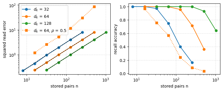
rng = np.random.default_rng(0)

def hebbian_memory(d, nums, num_values=256, trials=20, rho=0):
    """Read error and recall of S = sum_i k_i v_i^T over random unit keys;
    rho > 0 mixes every key with one shared direction (correlated keys)."""
    codebook = rng.standard_normal((num_values, d))
    codebook /= np.linalg.norm(codebook, axis=1, keepdims=True)
    errs, accs = [], []
    for n in nums:
        err = acc = 0
        for _ in range(trials):
            K = rng.standard_normal((n, d))
            K /= np.linalg.norm(K, axis=1, keepdims=True)  # Unit-norm keys
            if rho:                    # Break independence: shared component
                c = rng.standard_normal(d)
                K = np.sqrt(1 - rho ** 2) * K + rho * c / np.linalg.norm(c)
                K /= np.linalg.norm(K, axis=1, keepdims=True)
            ids = rng.integers(0, num_values, n)
            S = K.T @ codebook[ids]                        # Write: sum k v^T
            read = K @ S                                   # Rows are S^T k_j
            err += ((read - codebook[ids]) ** 2).sum(1).mean()
            acc += ((read @ codebook.T).argmax(1) == ids).mean()
        errs.append(err / trials)
        accs.append(acc / trials)
    return errs, accs

fig, axes = d2l.plt.subplots(1, 2, figsize=(9, 3.2))
for d in [32, 64, 128]:
    nums = [d // 4, d // 2, d, 2 * d, 4 * d, 8 * d]
    errs, accs = hebbian_memory(d, nums)
    axes[0].loglog(nums, errs, marker='o', label=f'$d_k$ = {d}')
    axes[0].loglog(nums, [(n - 1) / d for n in nums], 'k--', lw=1)
    axes[1].semilogx(nums, accs, marker='o', label=f'$d_k$ = {d}')
nums = [16, 32, 64, 128, 256, 512]                 # Width 64, correlated keys
errs, accs = hebbian_memory(64, nums, rho=0.5)
axes[0].loglog(nums, errs, marker='s', ls=':', color='C1',
               label=r'$d_k$ = 64, $\rho$ = 0.5')
axes[1].semilogx(nums, accs, marker='s', ls=':', color='C1')
for ax, ylabel in zip(axes, ['squared read error', 'recall accuracy']):
    ax.set_xlabel('stored pairs n')
    ax.set_ylabel(ylabel)
    ax.grid(linestyle='--', alpha=0.4)
axes[0].legend();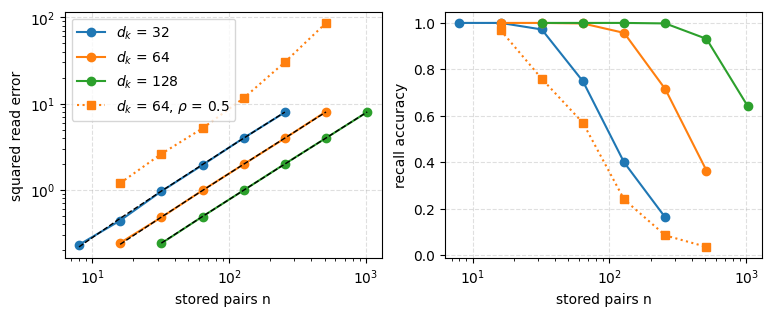
The left panel is the capacity law (both panels: independent isotropic unit keys, except the dotted curve): the measured error sits on the dashed \((n-1)/d_k\) prediction so closely that the curves are hard to tell apart, across a 256-fold range of \(n\) and three widths. The dotted curve breaks the proposition’s assumptions as promised, and the proposition’s cancellation is what it loses: with a common component in every key, the cross terms no longer vanish in expectation, the read error at \(d_k = 64\) sits about five-fold above the independent curve already at small \(n\) and grows faster than linearly, and recall degrades well before \(n\) reaches \(d_k\). Width stops helping when the keys all resemble one another; this is why the family normalizes its keys and why key geometry, not just key count, determines what a matrix memory holds. The right panel shows the corresponding recall accuracy. Recall is essentially perfect while the interference stays small relative to the unit-norm signal, then grows with \(n\) past \(d_k\); at a fixed error level, doubling the width doubles how many pairs fit. Nothing in either panel depends on when a pair was stored. This quantity controls the capacity comparison below: a fixed-size state does not lose memories to time, it loses them to crowding, and Section 12.7 will use this quantity when comparing how much full attention a production model must keep.
One caution about the word “capacity”, which this chapter uses for four distinct quantities. Algebraic rank: \(\mathbf{S}\) has rank at most \(d_k\), so no write rule stores more than \(d_k\) pairs with exact recall. Interference capacity: the proposition above, an expected read error under random independent keys. Information capacity: at finite precision, \(d_k d_v\) numbers hold at most a fixed number of bits, the counting behind the copying lower bound of Section 12.7. Task-usable capacity: what a trained model retrieves in practice, which Section 12.7 measures with its recall sweep and which none of the first three numbers guarantees.
12.4.1.2 Forms of Decay
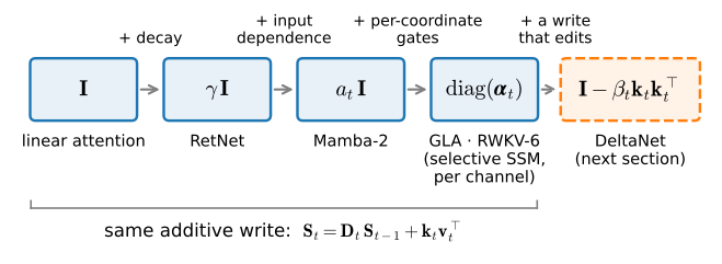
Decay limits crowding by shrinking preceding writes before each new write, preventing the interference sum from growing without bound. The family did this in three steps, each a one-line change to Equation 12.4.1:
\[ \mathbf{S}_t = \gamma\, \mathbf{S}_{t-1} + \mathbf{k}_t \mathbf{v}_t^\top, \qquad \mathbf{S}_t = a_t\, \mathbf{S}_{t-1} + \mathbf{k}_t \mathbf{v}_t^\top, \qquad \mathbf{S}_t = \mathrm{diag}(\boldsymbol{\alpha}_t)\, \mathbf{S}_{t-1} + \mathbf{k}_t \mathbf{v}_t^\top . \tag{12.4.4}\]
A fixed scalar \(\gamma \in (0,1)\) is RetNet’s retention (Sun et al. 2023): each head gets its own constant decay, so different heads keep different horizons. (If you worked the closing exercise of Section 10.5, you have already built this rung and verified that its parallel form weights past values by \(\gamma^{t-s}\).) An input-dependent scalar \(a_t\) is the transition of Mamba-2 (Dao and Gu 2024), one number per head per token. The token determines how much of the whole memory is retained, analogous to the forget gate of Section 12.1 applied to a matrix state. And an input-dependent diagonal \(\mathrm{diag}(\boldsymbol{\alpha}_t)\) decays each key coordinate at its own rate, the design of gated linear attention (GLA) (Yang, Wang, Shen, et al. 2024) and RWKV-6 (Peng et al. 2024). Figure 12.4.1 draws the ladder. The selective SSM of Section 12.3 lives on the diagonal rung too, run per channel: \(e^{\Delta_t \mathbf{a}}\) in Equation 12.3.2 is an input-dependent diagonal decay in everything but notation.
Each transition also has a statistical interpretation, which we note here and develop in Section 12.6. Stack the keys and values seen so far as rows of \(\mathbf{K}\) and \(\mathbf{V}\), and let the diagonal matrix \(\mathbf{W}\) hold each row’s accumulated decay. The linear read-out minimizing the decay-weighted squared error \(\sum_i w_i \|\mathbf{S}^\top \mathbf{k}_i - \mathbf{v}_i\|^2\) is the weighted least-squares solution
\[ \mathbf{S}^\star = \big(\mathbf{K}^\top \mathbf{W} \mathbf{K} + \lambda \mathbf{I}\big)^{-1} \mathbf{K}^\top \mathbf{W} \mathbf{V}, \tag{12.4.5}\]
with a small ridge \(\lambda\) (or a pseudoinverse at \(\lambda = 0\)) covering rank-deficient keys. The decayed state on any rung of the ladder stores only the weighted cross-moment \(\mathbf{K}^\top \mathbf{W} \mathbf{V}\): the shortcut that deletes the covariance correction \((\mathbf{K}^\top \mathbf{W} \mathbf{K} + \lambda \mathbf{I})^{-1}\). For orthonormal keys the deletion adds no error beyond the decay’s own discounting of each stored value; for overlapping keys it also incurs interference sum of Equation 12.4.2. The decay sets how fast old evidence expires, and which architectures restore the deleted correction is part of Section 12.6’s subject.
12.4.2 The State-Space Duality
We now connect this recurrence to Chapter 10. Take the scalar-decay transition, the simplest form with forgetting, and unroll it, exactly as we unrolled the LTI recurrence into a convolution in Section 12.2.3.2. Substituting the update into itself, the state at time \(t\) is a decayed sum of every write so far, and the read-out is
\[ \mathbf{o}_t = \sum_{s \le t} \big(a_t\, a_{t-1} \cdots a_{s+1}\big)\, (\mathbf{q}_t^\top \mathbf{k}_s)\, \mathbf{v}_s, \qquad \textrm{i.e.} \qquad \mathbf{Y} = \big(\mathbf{L} \circ \mathbf{Q}\mathbf{K}^\top\big)\, \mathbf{V}, \quad L_{ts} = \!\!\prod_{r=s+1}^{t}\!\! a_r, \tag{12.4.6}\]
where \(\circ\) is the elementwise product and \(\mathbf{L}\) is lower triangular with ones on the diagonal. The structure of \(\mathbf{L}\) establishes the equivalence. If every \(a_t = 1\), then \(L_{ts} = 1\) for \(t \ge s\) and zero otherwise: \(\mathbf{L}\) is the causal mask, and Equation 12.4.6 is masked linear attention, scores \(\mathbf{Q}\mathbf{K}^\top\), mask, value mixing, exactly as in Section 10.5. A gated linear recurrence is attention whose 0/1 causal mask has been replaced by a learned, decaying mask. These are two formulations of the same object. Dao and Gu (2024) named the correspondence state space duality (SSD), and matrices of \(\mathbf{L}\)’s form are called 1-semiseparable, every submatrix below the diagonal having rank one. The equivalence has a restricted scope: it is an identity for this structured family, a scalar-gated (1-semiseparable) mask on linear attention, not a statement about softmax attention, whose exponential kernel is no masked linear read.
The duality is also a statement about computation. The right-hand side of Equation 12.4.6 is a triple product, and the two ways of parenthesizing it are the two modes we already know. Materialize \(\mathbf{L} \circ \mathbf{Q}\mathbf{K}^\top\) first and you compute attention: quadratic in \(T\), all positions in parallel, no state in sight. Sweep the sum over \(s\) from the left instead, one \(t\) at a time, and the partial sums are the state \(\mathbf{S}_t\): linear in \(T\), constant memory, one token at a time. The two methods use different contraction orders for the same tensor. The following computation verifies their agreement, beginning with the recurrent form:
torch.manual_seed(0)
d_k, d_v, T = 64, 64, 512
device = d2l.try_gpu()

def matrix_state_recurrent(Q, K, V, a):
    """S_t = a_t S_{t-1} + k_t v_t^T, read o_t = S_t^T q_t."""
    S = Q.new_zeros(Q.shape[-1], V.shape[-1])
    outputs = []
    for t in range(Q.shape[0]):
        S = a[t] * S + K[t][:, None] * V[t][None, :]    # Decay, then write
        outputs.append(Q[t] @ S)                        # Read S^T q
    return torch.stack(outputs)

Q, K, V = (torch.randn(T, d, device=device) for d in (d_k, d_k, d_v))
a = 0.65 + 0.3 * torch.rand(T, device=device)           # Decays in (0.65, 0.95)
y_rec = matrix_state_recurrent(Q, K, V, a)
d_k, d_v, T = 64, 64, 512
def matrix_state_recurrent(Q, K, V, a):
"""S_t = a_t S_{t-1} + k_t v_t^T, read o_t = S_t^T q_t."""
def step(S, qkva):
q, k, v, a_t = qkva
S = a_t * S + k[:, None] * v[None, :] # Decay, then write
return S, q @ S # Read S^T q
S0 = jnp.zeros((Q.shape[-1], V.shape[-1]))
return jax.lax.scan(step, S0, (Q, K, V, a))[1]
keys = jax.random.split(jax.random.key(0), 4)
Q, K, V = (jax.random.normal(k, (T, d))
for k, d in zip(keys, (d_k, d_k, d_v)))
a = 0.65 + 0.3 * jax.random.uniform(keys[3], (T,)) # Decays in (0.65, 0.95)
y_rec = matrix_state_recurrent(Q, K, V, a)The quadratic dual builds \(\mathbf{L}\) in log space: the product of decays from \(s\) to \(t\) is a difference of cumulative log-decays, and masking with \(-\infty\) before exponentiating keeps the entries above the diagonal from overflowing (they would be products of inverse decays). We assert agreement rather than eyeball it; this check is the duality.
def matrix_state_dual(Q, K, V, a):
    """Y = (L o Q K^T) V with L_ts = a_t ... a_{s+1} for t >= s, else 0."""
    cum = torch.cumsum(torch.log(a), 0)
    logL = cum[:, None] - cum[None, :]                  # Sum of logs over (s, t]
    causal = torch.tril(torch.ones(len(a), len(a), dtype=torch.bool,
                                   device=a.device))
    L = torch.exp(logL.masked_fill(~causal, -torch.inf))
    return (L * (Q @ K.T)) @ V

err = (matrix_state_dual(Q, K, V, a) - y_rec).abs().max() / y_rec.abs().max()
print(f'relative deviation, dual vs recurrence: {float(err):.2e}')
assert err < 1e-3                          # Two orders, one computation

ones = torch.ones(T, device=device)                     # All a_t = 1
err = (matrix_state_dual(Q, K, V, ones)
       - torch.tril(Q @ K.T) @ V).abs().max()
print(f'a_t = 1, deviation from masked linear attention: {float(err):.2e}')
assert err < 1e-6                          # L is literally the causal mask
relative deviation, dual vs recurrence: 5.11e-06
a_t = 1, deviation from masked linear attention: 0.00e+00def matrix_state_dual(Q, K, V, a):
"""Y = (L o Q K^T) V with L_ts = a_t ... a_{s+1} for t >= s, else 0."""
cum = jnp.cumsum(jnp.log(a))
logL = cum[:, None] - cum[None, :] # Sum of logs over (s, t]
causal = jnp.tril(jnp.ones((len(a), len(a)), bool))
L = jnp.exp(jnp.where(causal, logL, -jnp.inf))
return (L * (Q @ K.T)) @ V
with jax.default_matmul_precision('highest'):
err = (jnp.abs(matrix_state_dual(Q, K, V, a) - y_rec).max()
/ jnp.abs(y_rec).max())
print(f'relative deviation, dual vs recurrence: {float(err):.2e}')
assert err < 1e-3 # Two orders, one computation
ones = jnp.ones(T) # All a_t = 1
err = jnp.abs(matrix_state_dual(Q, K, V, ones)
- jnp.tril(Q @ K.T) @ V).max()
print(f'a_t = 1, deviation from masked linear attention: {float(err):.2e}')
assert err < 1e-6 # L is literally the causal maskrelative deviation, dual vs recurrence: 4.14e-06
a_t = 1, deviation from masked linear attention: 0.00e+00Ten lines of quadratic code, a scan-shaped loop, and they agree to floating-point rounding; with the decays pinned to one, the dual reduces exactly to the masked linear attention of Chapter 10. The correspondence that Section 10.5 promised is now a computation you have run, not an analogy. It also locates Mamba-2 precisely: take Section 12.3’s selective model, restrict its per-coordinate decay to a single input-dependent scalar per head, and the layer is Equation 12.4.6, trainable in whichever mode is cheaper. The recurrence costs \(\mathcal{O}(T)\) but executes sequentially, whereas the dual is parallel but costs \(\mathcal{O}(T^2)\). Chunking provides an intermediate schedule.
12.4.3 Chunked Computation: Mostly Matmul, a Little Scan
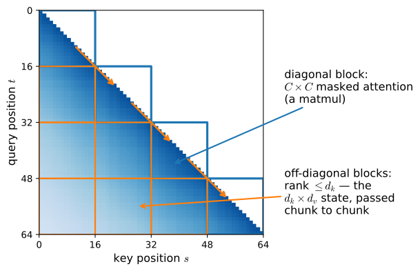
There is, and it is how GLA, Mamba-2, and the DeltaNet family of the next section all train. Partition the sequence into chunks of \(C\) tokens and partition \(\mathbf{L} \circ \mathbf{Q}\mathbf{K}^\top\) accordingly, as in Figure 12.4.2. The blocks on the diagonal are the interactions within a chunk: each is a \(C \times C\) masked-attention product, quadratic only in the chunk length, and all of them run in parallel. Everything below the diagonal is the influence of earlier chunks on later ones, and here the semiseparable structure pays off: those blocks have rank at most \(d_k\), because all a later chunk needs from the entire past is the \(d_k \times d_v\) state at its boundary. The algorithm computes the diagonal blocks as matmuls, passes the state between chunks with a recurrence of \(T/C\) steps, and adds each chunk’s read of its incoming state. It therefore uses attention within chunks and recurrence across chunks (Dao and Gu 2024).
The implementation needs one helper. segsum builds, for one chunk, the matrix of segment sums of log-decays, \(\sum_{s < r \le t} \log a_r\), whose exponential is the within-chunk \(\mathbf{L}\); as in the dual, the invalid upper triangle is masked to \(-\infty\) in log space, before any exponential can overflow. The chunked form is then a dozen lines: the decayed attention matmul inside each chunk, and a loop over chunk boundaries that carries the state, decays each key’s write to its chunk’s end, and lets each chunk read the state it inherited.
def segsum(log_a):
    """Segment sums: (..., C) -> (..., C, C) with entries sum over (s, t]."""
    C = log_a.shape[-1]
    cum = torch.cumsum(log_a, -1)
    diff = cum[..., :, None] - cum[..., None, :]
    keep = torch.tril(torch.ones(C, C, dtype=torch.bool, device=log_a.device))
    return diff.masked_fill(~keep, -torch.inf)          # Mask in log space

def matrix_state_chunked(Q, K, V, a, chunk_size=64):
    """The same Y, chunk by chunk: attention inside, recurrence across."""
    T, C = Q.shape[0], chunk_size
    Qc, Kc = Q.view(-1, C, Q.shape[-1]), K.view(-1, C, K.shape[-1])
    Vc, log_a = V.view(-1, C, V.shape[-1]), torch.log(a).view(-1, C)
    L = torch.exp(segsum(log_a))                        # (T/C, C, C)
    b = torch.exp(torch.cumsum(log_a, -1))              # Decay since chunk entry
    Y = (L * (Qc @ Kc.transpose(-1, -2))) @ Vc          # Diagonal blocks
    S = Q.new_zeros(Q.shape[-1], V.shape[-1])
    for c in range(T // C):                             # T/C boundary steps
        Y[c] += (Qc[c] * b[c][:, None]) @ S             # Read the carried state
        S = b[c][-1] * S + (Kc[c] * (b[c][-1] / b[c])[:, None]).T @ Vc[c]
    return Y.reshape(T, -1)

for chunk_size in [16, 64, 256]:
    err = ((matrix_state_chunked(Q, K, V, a, chunk_size) - y_rec).abs().max()
           / y_rec.abs().max())
    print(f'chunk size {chunk_size:4d}: relative deviation {float(err):.2e}')
    assert err < 1e-3                      # Chunked == recurrence
chunk size 16: relative deviation 1.92e-07
chunk size 64: relative deviation 6.81e-07
chunk size 256: relative deviation 1.75e-06def segsum(log_a):
"""Segment sums: (..., C) -> (..., C, C) with entries sum over (s, t]."""
C = log_a.shape[-1]
cum = jnp.cumsum(log_a, -1)
diff = cum[..., :, None] - cum[..., None, :]
keep = jnp.tril(jnp.ones((C, C), bool))
return jnp.where(keep, diff, -jnp.inf) # Mask in log space
def matrix_state_chunked(Q, K, V, a, chunk_size=64):
"""The same Y, chunk by chunk: attention inside, recurrence across."""
T, C = Q.shape[0], chunk_size
Qc, Kc = Q.reshape(-1, C, Q.shape[-1]), K.reshape(-1, C, K.shape[-1])
Vc, log_a = V.reshape(-1, C, V.shape[-1]), jnp.log(a).reshape(-1, C)
L = jnp.exp(segsum(log_a)) # (T/C, C, C)
b = jnp.exp(jnp.cumsum(log_a, -1)) # Decay since chunk entry
Y = (L * (Qc @ Kc.transpose(0, 2, 1))) @ Vc # Diagonal blocks
def boundary(S, chunk): # T/C boundary steps
Qb, Kb, Vb, bb, Yb = chunk
Yb = Yb + (Qb * bb[:, None]) @ S # Read the carried state
S = bb[-1] * S + (Kb * (bb[-1] / bb)[:, None]).T @ Vb
return S, Yb
S0 = jnp.zeros((Q.shape[-1], V.shape[-1]))
_, Y = jax.lax.scan(boundary, S0, (Qc, Kc, Vc, b, Y))
return Y.reshape(T, -1)
with jax.default_matmul_precision('highest'):
for chunk_size in [16, 64, 256]:
err = (jnp.abs(matrix_state_chunked(Q, K, V, a, chunk_size)
- y_rec).max() / jnp.abs(y_rec).max())
print(f'chunk size {chunk_size:4d}: relative deviation {float(err):.2e}')
assert err < 1e-3 # Chunked == recurrencechunk size 16: relative deviation 2.13e-07
chunk size 64: relative deviation 3.84e-07
chunk size 256: relative deviation 1.54e-06One numerical note before we time these forms. Within a chunk, segsum works in log space and masks with \(-\infty\) before exponentiating, so the diagonal blocks cannot overflow. The boundary step is less careful: it exponentiates the prefix products \(b\) and then divides, and \(b\) shrinks geometrically with position in the chunk. For our decay range the smallest prefix product at \(C = 256\) is around \(10^{-28}\), still inside float32’s range; by \(C = 512\) it underflows to exactly zero and the late-chunk ratios \(b_C / b_t\) degenerate to \(0/0\). The \(C = 1024\) row of the timing table below therefore measures the right arithmetic shape — the work and memory traffic are unchanged — on values that have already turned to NaN; correctness holds for the chunk sizes asserted above. Production kernels carry the boundary decays in log space too, or rescale chunk by chunk, for exactly this reason; we keep the plain ratio because it leaves the algebra visible.
The chunk size interpolates between the two modes we proved dual: at \(C = 1\) each diagonal block shrinks to the \(1 \times 1\) self-write \((\mathbf{q}_t^\top \mathbf{k}_t)\,\mathbf{v}_t\) — within-chunk interaction between distinct tokens is gone, and everything earlier flows through the state recurrence; at \(C = T\) there is one block and no recurrence. The preferred chunk size depends on both time and memory, so we measure each as in the attention experiments of Section 10.5.
T = 4096
Q, K, V = (torch.randn(T, d, device=device) for d in (d_k, d_k, d_v))
a = 0.65 + 0.3 * torch.rand(T, device=device)

def wall_clock(f, *args, reps=5):
    f(*args)  # Warm up
    if device.type == 'cuda':
        torch.cuda.synchronize()
    start = time.time()
    for _ in range(reps):
        f(*args)
    if device.type == 'cuda':
        torch.cuda.synchronize()
    return (time.time() - start) / reps

def peak_memory(f, *args):
    """Extra peak memory allocated by f, in bytes (CUDA only)."""
    torch.cuda.synchronize()
    torch.cuda.reset_peak_memory_stats()
    base = torch.cuda.memory_allocated()
    f(*args)
    torch.cuda.synchronize()
    return torch.cuda.max_memory_allocated() - base

forms = {'recurrence': matrix_state_recurrent}
for C in [16, 64, 256, 1024]:
    forms[f'chunked ({C})'] = \
        lambda q, k, v, a, C=C: matrix_state_chunked(q, k, v, a, C)
forms['quadratic dual'] = matrix_state_dual

print(f'{"form":>15} {"time (ms)":>10} {"peak (MiB)":>11}')
for name, f in forms.items():
    t = wall_clock(f, Q, K, V, a) * 1e3
    mem = (f'{peak_memory(f, Q, K, V, a) / 2**20:11.1f}'
           if device.type == 'cuda' else f'{"n/a":>11}')
    print(f'{name:>15} {t:10.2f} {mem}')
dev = torch.cuda.get_device_name(device) if device.type == 'cuda' else 'CPU'
print(f'({dev}, float32, torch {torch.__version__}; '
      f'teaching implementations, warmed up)')
form time (ms) peak (MiB)
recurrence 282.93 3.0
chunked (16) 36.12 1.5
chunked (64) 9.42 3.0
chunked (256) 2.61 12.0
chunked (1024) 0.87 48.0
quadratic dual 1.01 272.0
(NVIDIA GeForce RTX 4090, float32, torch 2.11.0+cu128; teaching implementations, warmed up)T = 4096
keys = jax.random.split(jax.random.key(1), 4)
Q, K, V = (jax.random.normal(k, (T, d))
for k, d in zip(keys, (d_k, d_k, d_v)))
a = 0.65 + 0.3 * jax.random.uniform(keys[3], (T,))
def wall_clock(f, *args, reps=5):
f(*args).block_until_ready() # Warm up (and compile)
start = time.time()
for _ in range(reps):
f(*args).block_until_ready()
return (time.time() - start) / reps
forms = {'recurrence': jax.jit(matrix_state_recurrent)}
for C in [16, 64, 256, 1024]:
forms[f'chunked ({C})'] = jax.jit(
lambda q, k, v, a, C=C: matrix_state_chunked(q, k, v, a, C))
forms['quadratic dual'] = jax.jit(matrix_state_dual)
print(f'{"form":>15} {"time (ms)":>10} {"temp (MiB)":>11}')
for name, f in forms.items():
stats = f.lower(Q, K, V, a).compile().memory_analysis()
print(f'{name:>15} {wall_clock(f, Q, K, V, a) * 1e3:10.2f} '
f'{stats.temp_size_in_bytes / 2**20:11.1f}')
print(f'({jax.devices()[0].device_kind}, float32, jax {jax.__version__}; '
f'teaching implementations, all forms compiled)') form time (ms) temp (MiB)
recurrence 49.63 0.0
chunked (16) 2.80 1.1
chunked (64) 1.62 1.1
chunked (256) 0.46 5.0
chunked (1024) 0.37 21.0
quadratic dual 0.45 68.0
(NVIDIA GeForce RTX 4090, float32, jax 0.10.2; teaching implementations, all forms compiled)Provenance first: these are our teaching implementations, timed in float32 on the printed device after a warm-up pass, and the two frameworks do not measure quite the same thing — the PyTorch recurrence is an eager Python loop paying per-step dispatch, while JAX compiles all three forms, which flatters the recurrence. Read the orders of magnitude, not the exact ratios. The pattern in our runs is the one the derivation predicts. The token recurrence is by far the slowest, a couple of orders of magnitude behind the best schedule: its \(T\) steps are serialized, whether as eager kernel launches or as a compiled scan, so the accelerator’s parallelism sits unused, though its memory footprint is trivial. The quadratic dual is the mirror image: matmul-fast, but its \(T \times T\) matrices dominate the memory column and grow fourfold with every doubling of \(T\). With chunks of a few hundred tokens, the chunked schedule runs within a small factor of the dual’s speed, and sometimes faster in these runs, while using an order of magnitude less memory. Its principal operations are dense matmuls that use the accelerator efficiently. Chunks up to \(C \approx d_k\) keep the arithmetic within a small factor of the recurrence’s, as an exercise asks you to derive; the measured optimum sits at larger chunks because kernel-launch overhead penalizes many small ones.
12.4.3.1 Measured Performance
Mamba-2 differs from Mamba primarily in its computational schedule rather than its model class. Recall from Section 10.5 that an accelerator moves bytes far more slowly than it multiplies them; its full arithmetic rate is reserved for dense matrix products on tensor cores. Mamba-1’s parallel scan is elementwise work, so it runs at memory bandwidth and leaves the matmul units idle. Restricting the transition to a scalar per head buys the chunked form above, whose inner loop uses matmuls. The Mamba-2 paper reports that this schedule made training several times faster while allowing the state dimension to increase from \(N = 16\) to \(64\)–\(256\) with little additional wall-clock time, because a larger state produces better-shaped matmuls for the hardware (Dao and Gu 2024). The capacity law of Section 12.4.1.1 says what that buys: an order of magnitude more pairs held at the same read error. The trade is not one-sided, and it runs in both directions: Mamba-1’s per-coordinate decay is a more expressive transition per unit of state, and for pure recurrent inference, where there are no chunks and every step is elementwise either way, nothing forces the scalar restriction. Production systems pick per workload. The frontier keeps moving on the same axis: Mamba-3 upgrades the discretization itself, replacing the Euler-style update on the input path with a trapezoidal rule (and adding complex-valued states and multi-input, multi-output reads that feed the decode-time matmuls) (Lahoti et al. 2026).
One accounting cell closes the systems thread that Section 11.3 opened. A transformer’s per-layer cache grows linearly with context; every matrix state in this section is a constant. Priced per layer and per sequence, at \(b\) bytes per element, the two sides of the ledger are
\[ \underbrace{\big(d_{\textrm{inner}}\, d_{\textrm{state}} + d_{\textrm{inner}}\, (w - 1)\big)\, b}_{\textrm{recurrent: SSM state + conv buffer, constant}} \qquad \textrm{vs.} \qquad \underbrace{2\, n\, h_{\textrm{kv}}\, d_{\textrm{head}}\, b}_{\textrm{KV cache, grows with the } n \textrm{ tokens kept}}, \tag{12.4.7}\]
where \(w\) is the causal-convolution width whose rolling buffer decoding must also carry (Section 12.3.3.2) and \(h_{\textrm{kv}}\) the number of KV heads; a batch multiplies both sides by its size, and a whole model multiplies both by its layer count. The cell prices the \(64 \times 64\) head state of our cells and one fully specified production instance — a Mamba-2 2.7B layer: \(d_{\textrm{model}} = 2560\), expansion \(2\), so \(d_{\textrm{inner}} = 5120\), \(d_{\textrm{state}} = 128\), \(w = 4\), hence \(5120 \times 128 = 655{,}360\) state elements per layer — against the grouped-query KV settings of Section 11.3. Headline numbers use fp16 (\(b = 2\)) on both sides, the common serving precision; the formula re-prices any row for other dtypes.
def mib(elements, bytes_per=2):             # fp16 headline; re-price at will
    return elements * bytes_per / 2**20

d_inner, d_state, w = 5120, 128, 4          # Mamba-2 2.7B layer
ssm, conv = d_inner * d_state, d_inner * (w - 1)
print('per layer, per sequence, fp16:')
print(f'matrix state, one 64x64 head:  {mib(64 * 64):8.2f} MiB, constant')
print(f'Mamba-2 2.7B, SSM {ssm:,} + conv {conv:,} elements: '
      f'{mib(ssm + conv):.2f} MiB, constant')
for n in [4096, 131072, 1048576]:
    kv = 2 * n * 8 * 128                    # 2 x tokens x kv-heads x head-dim
    print(f'GQA KV cache at n = {n:>9,}: {mib(kv):8.2f} MiB and growing')
per layer, per sequence, fp16:
matrix state, one 64x64 head: 0.01 MiB, constant
Mamba-2 2.7B, SSM 655,360 + conv 15,360 elements: 1.28 MiB, constant
GQA KV cache at n = 4,096: 16.00 MiB and growing
GQA KV cache at n = 131,072: 512.00 MiB and growing
GQA KV cache at n = 1,048,576: 4096.00 MiB and growingdef mib(elements, bytes_per=2): # fp16 headline; re-price at will
return elements * bytes_per / 2**20
d_inner, d_state, w = 5120, 128, 4 # Mamba-2 2.7B layer
ssm, conv = d_inner * d_state, d_inner * (w - 1)
print('per layer, per sequence, fp16:')
print(f'matrix state, one 64x64 head: {mib(64 * 64):8.2f} MiB, constant')
print(f'Mamba-2 2.7B, SSM {ssm:,} + conv {conv:,} elements: '
f'{mib(ssm + conv):.2f} MiB, constant')
for n in [4096, 131072, 1048576]:
kv = 2 * n * 8 * 128 # 2 x tokens x kv-heads x head-dim
print(f'GQA KV cache at n = {n:>9,}: {mib(kv):8.2f} MiB and growing')per layer, per sequence, fp16:
matrix state, one 64x64 head: 0.01 MiB, constant
Mamba-2 2.7B, SSM 655,360 + conv 15,360 elements: 1.28 MiB, constant
GQA KV cache at n = 4,096: 16.00 MiB and growing
GQA KV cache at n = 131,072: 512.00 MiB and growing
GQA KV cache at n = 1,048,576: 4096.00 MiB and growingThe recurrent side of the ledger is constant in context length; the cache side crosses it within a few thousand tokens and keeps growing with every token kept. Both sides compose with quantization, and the cache side with sharing and eviction schemes, so the constants move; the shapes do not. What the flat line costs, we measured at the start of this section: a capacity ceiling set by the state’s width. Holding both numbers in mind at once is the whole hybrid-design problem of Section 12.7, which prices whole models with exactly Equation 12.4.7.
12.4.4 Model Family
The models in this section and its two predecessors are instances of Equation 12.4.1. In the table below, the transition column compares decay structures, and the write column is uniform by design.
Reading the papers. The literature does not agree on which way the state matrix points. Katharopoulos et al. (2020) write \(\mathbf{S} = \sum_s \phi(\mathbf{k}_s)\mathbf{v}_s^\top\) read by \(\phi(\mathbf{q})^\top \mathbf{S}\), as we do; RetNet and GLA carry the same state under transposed notation; the DeltaNet line stores the transpose \(\mathbf{S} \in \mathbb{R}^{d_v \times d_k}\), writes \(\mathbf{v}_t \mathbf{k}_t^\top\), and applies transitions from the right. All of these are one recurrence up to transposition. This chapter fixes a single convention, keys index rows: \(\mathbf{S}_t = \mathbf{D}_t \mathbf{S}_{t-1} + \mathbf{k}_t \mathbf{v}_t^\top\) with read \(\mathbf{o}_t = \mathbf{S}_t^\top \mathbf{q}_t\), and translates every paper into it, as in Table 12.4.1.
| model | state | transition \(\mathbf{D}_t\) | write | update interpretation |
|---|---|---|---|---|
| linear attention (2020) | \(\mathbf{S}\) and normalizer \(\mathbf{z}\) | \(\mathbf{I}\) | add \(\phi(\mathbf{k}_t)\mathbf{v}_t^\top\) | attention minus softmax |
| RetNet (2023) | \(\mathbf{S}\) per head | \(\gamma\,\mathbf{I}\), fixed per head | add \(\mathbf{k}_t\mathbf{v}_t^\top\) | linear attention plus decay |
| Mamba (2023) | vector \(\mathbf{x}_t \in \mathbb{R}^N\) per channel | input-dep. diagonal \(e^{\Delta_t \mathbf{a}}\) | add \(\Delta_t u_t \mathbf{B}_t\) | selective SSM (Section 12.3) |
| GLA (2024) | \(\mathbf{S}\) per head | input-dep. diagonal \(\mathrm{diag}(\boldsymbol{\alpha}_t)\) | add \(\mathbf{k}_t\mathbf{v}_t^\top\) | per-coordinate forgetting |
| Mamba-2 (2024) | \(\mathbf{S}\) per head | input-dep. scalar \(a_t\,\mathbf{I}\) | add \(\mathbf{k}_t\mathbf{v}_t^\top\) | the duality of this section |
| RWKV-6 (2024) | \(\mathbf{S}\) per head | input-dep. diagonal \(\mathrm{diag}(\mathbf{w}_t)\) | add \(\mathbf{k}_t\mathbf{v}_t^\top\) | the RNN lineage arrives |
| mLSTM (2024) | \(\mathbf{S}\) and normalizer \(\mathbf{z}\) | scalar gate \(f_t\,\mathbf{I}\) | add \(i_t\,\mathbf{k}_t\mathbf{v}_t^\top\) | LSTM with a matrix cell |
Three research lineages fill the rows: attention seeking linearity (linear attention, RetNet, GLA), state space models seeking selectivity (Mamba, Mamba-2), and recurrent networks seeking parallelism (RWKV-6, mLSTM). That they converge on one recurrence is the strongest evidence in this book that the recurrence, rather than any single architecture, is the right object of study. Mamba’s row is the one non-matrix entry: its per-channel vector state is the same mathematics run single-input, single-output, and Mamba-2’s move to the matrix state is what the duality section derived.
12.4.4.1 The One That Kept the Normalizer
The last row retains the normalizer \(\mathbf{z}\) introduced in Chapter 10. The mLSTM is the matrix-memory cell of xLSTM (Beck et al. 2024), the LSTM rebuilt on Equation 12.4.1: a forget gate \(f_t\) and input gate \(i_t\), computed from the token, gating a matrix cell state and, alongside it, the running normalizer that the rest of the family traded for output normalization:
\[ \mathbf{S}_t = f_t\, \mathbf{S}_{t-1} + i_t\, \mathbf{k}_t \mathbf{v}_t^\top, \qquad \mathbf{z}_t = f_t\, \mathbf{z}_{t-1} + i_t\, \mathbf{k}_t, \qquad \mathbf{o}_t = \frac{\mathbf{S}_t^\top \mathbf{q}_t} {\max\big(|\mathbf{z}_t^\top \mathbf{q}_t|,\, 1\big)}, \tag{12.4.8}\]
with \(i_t = \exp(\tilde{i}_t)\) and \(f_t = \sigma(\tilde{f}_t)\) or \(\exp(\tilde{f}_t)\) for learned pre-activations \(\tilde{i}_t, \tilde{f}_t\) (the paper’s \(\mathbf{C}_t\) and \(\mathbf{n}_t\) are our \(\mathbf{S}_t\) and \(\mathbf{z}_t\) transposed). The exponential gates are the novelty and the hazard: they let a single strong token outweigh the entire accumulated past, and they overflow float32 after a few dozen steps of ordinary gate values. The fix is one we have already met. Exactly as online softmax Equation 10.5.2 carries a running maximum and rescales the past, the mLSTM carries a stabilizer state \(m_t\) (Milakov and Gimelshein 2018):
\[ m_t = \max\big(\tilde{f}_t + m_{t-1},\, \tilde{i}_t\big), \qquad f'_t = \exp\big(\tilde{f}_t + m_{t-1} - m_t\big), \qquad i'_t = \exp\big(\tilde{i}_t - m_t\big), \tag{12.4.9}\]
for the exponential-forget case. Running the recurrence with \((f'_t, i'_t)\) scales state and normalizer by the same factor \(e^{-m_t}\), so the read-out is unchanged provided the constant \(1\) in the denominator is scaled too, to \(e^{-m_t}\). We implement the recurrence directly from these equations (the reference xLSTM code base is under a restrictive license, so reimplementing from the paper is also the legally clean route) and verify both claims at once: the unstabilized float32 recurrence dies, and the stabilized one matches an unstabilized float64 reference to float precision.
torch.manual_seed(0)
d_k, d_v, T = 8, 8, 64
q, k, v = (torch.randn(T, d) for d in (d_k, d_k, d_v))
i_pre, f_pre = torch.randn(T), 2.0 + torch.randn(T)  # Gate pre-activations

def mlstm_naive(q, k, v, i_pre, f_pre, dtype):
    """The unstabilized recurrence, in a given precision."""
    q, k, v = q.to(dtype), k.to(dtype), v.to(dtype)
    i_g, f_g = i_pre.to(dtype).exp(), f_pre.to(dtype).exp()
    S, z = torch.zeros(d_k, d_v, dtype=dtype), torch.zeros(d_k, dtype=dtype)
    outputs = []
    for t in range(T):
        S = f_g[t] * S + i_g[t] * (k[t][:, None] * v[t][None, :])
        z = f_g[t] * z + i_g[t] * k[t]
        outputs.append(q[t] @ S / (q[t] @ z).abs().clamp(min=1))
    return torch.stack(outputs)

def mlstm_stabilized(q, k, v, i_pre, f_pre):
    """Carry m_t and rescale the past, as in online softmax."""
    S, z = torch.zeros(d_k, d_v), torch.zeros(d_k)
    m = torch.tensor(-torch.inf)
    outputs = []
    for t in range(T):
        m_new = torch.maximum(f_pre[t] + m, i_pre[t])
        f_g, i_g = torch.exp(f_pre[t] + m - m_new), torch.exp(i_pre[t] - m_new)
        S = f_g * S + i_g * (k[t][:, None] * v[t][None, :])
        z = f_g * z + i_g * k[t]
        m = m_new
        outputs.append(q[t] @ S
                       / torch.maximum((q[t] @ z).abs(), torch.exp(-m)))
    return torch.stack(outputs)

exact = mlstm_naive(q, k, v, i_pre, f_pre, torch.float64)
naive = mlstm_naive(q, k, v, i_pre, f_pre, torch.float32)
bad = ~torch.isfinite(naive).all(-1)        # argmax(bool) would report 0
first_bad = int(bad.float().argmax()) if bool(bad.any()) else 'none'
stab = mlstm_stabilized(q, k, v, i_pre, f_pre)
err = (stab - exact.float()).abs().max() / exact.abs().max()
print(f'float32 unstabilized: first non-finite output at step {first_bad}')
print(f'float32 stabilized vs float64: relative deviation {float(err):.2e}')
assert torch.isfinite(stab).all() and err < 1e-3
float32 unstabilized: first non-finite output at step 49
float32 stabilized vs float64: relative deviation 2.02e-05d_k, d_v, T = 8, 8, 64
kk = jax.random.split(jax.random.key(2), 5)
q, k, v = (jax.random.normal(key, (T, d))
for key, d in zip(kk, (d_k, d_k, d_v)))
i_pre = jax.random.normal(kk[3], (T,)) # Gate pre-activations
f_pre = 2.0 + jax.random.normal(kk[4], (T,))
def mlstm_naive(q, k, v, i_pre, f_pre, dtype):
"""The unstabilized recurrence (NumPy), in a given precision."""
q, k, v = (np.asarray(x, dtype) for x in (q, k, v))
i_g, f_g = np.exp(np.asarray(i_pre, dtype)), np.exp(np.asarray(f_pre, dtype))
S, z = np.zeros((d_k, d_v), dtype), np.zeros(d_k, dtype)
outputs = []
for t in range(T):
S = f_g[t] * S + i_g[t] * np.outer(k[t], v[t])
z = f_g[t] * z + i_g[t] * k[t]
outputs.append(q[t] @ S / max(abs(q[t] @ z), 1.0))
return np.stack(outputs)
def mlstm_stabilized(q, k, v, i_pre, f_pre):
"""Carry m_t and rescale the past, as in online softmax."""
def step(carry, x):
S, z, m = carry
q_t, k_t, v_t, i_t, f_t = x
m_new = jnp.maximum(f_t + m, i_t)
f_g, i_g = jnp.exp(f_t + m - m_new), jnp.exp(i_t - m_new)
S = f_g * S + i_g * (k_t[:, None] * v_t[None, :])
z = f_g * z + i_g * k_t
o = q_t @ S / jnp.maximum(jnp.abs(q_t @ z), jnp.exp(-m_new))
return (S, z, m_new), o
init = (jnp.zeros((d_k, d_v)), jnp.zeros(d_k), -jnp.inf)
return jax.lax.scan(step, init, (q, k, v, i_pre, f_pre))[1]
exact = mlstm_naive(q, k, v, i_pre, f_pre, np.float64)
with np.errstate(over='ignore', invalid='ignore'): # The overflow is the point
naive = mlstm_naive(q, k, v, i_pre, f_pre, np.float32)
bad = ~np.isfinite(naive).all(-1) # argmax(bool) would report 0
first_bad = int(bad.argmax()) if bad.any() else 'none'
stab = mlstm_stabilized(q, k, v, i_pre, f_pre)
err = jnp.abs(stab - exact).max() / jnp.abs(exact).max()
print(f'float32 unstabilized: first non-finite output at step {first_bad}')
print(f'float32 stabilized vs float64: relative deviation {float(err):.2e}')
assert bool(jnp.isfinite(stab).all()) and err < 1e-3float32 unstabilized: first non-finite output at step 47
float32 stabilized vs float64: relative deviation 1.38e-06The mLSTM is one half of the xLSTM architecture; its scalar sibling sLSTM keeps the LSTM’s recurrent memory mixing (and therefore steps sequentially, gaining state-tracking power the parallel family lacks), a trade we noted in the gate table of Section 12.1.
12.4.4.2 Limitations of Additive Writes
Look down the write column of Table 12.4.1 once more. Seven models, three lineages, and every single write is an addition: not one model in the table can change what it wrote about key \(\mathbf{k}\) without also decaying everything else it knows. The decay ladder manages crowding, it does not cure it, because forgetting is indiscriminate where interference Equation 12.4.2 is specific. The fast weight programmers saw this in the 1990s and proposed the repair (Schlag et al. 2021): before writing to key \(\mathbf{k}_t\), first read what the memory already holds there, and write only the correction. That single change to the write rule is the subject of Section 12.5: a memory that edits rather than accumulates.
12.4.5 Summary
Linear attention’s matrix state and the selective SSM’s recurrence are one template, \(\mathbf{S}_t = \mathbf{D}_t \mathbf{S}_{t-1} + \mathbf{k}_t \mathbf{v}_t^\top\) read by the query. As a memory it has a measured capacity law: after \(n\) writes with independent isotropic unit keys into width \(d_k\), the expected squared read error is \((n-1)/d_k\) — and measurably worse once keys correlate — so capacity is set by width, not by time. The decay ladder adds forgetting one line at a time: fixed scalar (RetNet), input-dependent scalar (Mamba-2), input-dependent diagonal (GLA, RWKV-6, and per channel the selective SSM). Unrolling the scalar-decay recurrence gives \(\mathbf{Y} = (\mathbf{L} \circ \mathbf{Q}\mathbf{K}^\top)\mathbf{V}\) with a 1-semiseparable \(\mathbf{L}\); at \(a_t = 1\) the mask \(\mathbf{L}\) is literally the causal mask, so masked linear attention and the gated recurrence are the same matrix, and the quadratic and recurrent modes are two orders of one contraction. That is Mamba-2’s state space duality, verified here by assertion, and the family trains in the chunked middle order: attention within chunks, a short state recurrence across them, matmul-heavy and linear in sequence length, the schedule the Mamba-2 paper credits for growing state sizes an order of magnitude at little wall-clock cost. The family table collects the members, including the mLSTM, which keeps the normalizer state of Chapter 10 and stabilizes its exponential gates with the online-softmax rescaling. Every write rule in the table only adds; editing the memory is next.
Experimental scope. The capacity law is a proposition under independent isotropic random keys, confirmed by measurement under exactly those assumptions and shown failing under correlated keys; it bounds nothing about trained or whitened key geometries. The duality and chunking checks are identities for the scalar-gated family, verified to float tolerance. The timing and memory tables are illustrations from one device, dtype, and teaching implementation: constants that move across hardware and kernels around asymptotic shapes that do not.
12.4.6 Exercises
- Correlated keys. ● The call of
hebbian_memorywithrho=0.5in Section 12.4.1.1 builds each key by normalizing \(\sqrt{1-\rho^2}\, \mathbf{g}_i + \rho\, \mathbf{c}\), where the \(\mathbf{g}_i\) are independent isotropic unit vectors and \(\mathbf{c}\) is one shared unit vector. Model the overlap of two distinct keys as \(\mathbf{k}_i^\top \mathbf{k}_j = \rho^2 + \epsilon_{ij}\). For fixed \(j\), let the \(\epsilon_{ij}\) with \(i \neq j\) be independent of each other and of the values, with mean zero and variance \(\sigma^2 = (1-\rho^2)^2 / d_k\). This model keeps the shared component and the term \((1-\rho^2)\, \mathbf{g}_i^\top \mathbf{g}_j\), and it neglects the renormalization and the terms linear in \(\rho\). The stored values have unit norm and are independent of the keys.- Assume that the values are also independent of each other with mean zero. Derive the expected squared read error at key \(j\), which generalizes Equation 12.4.3, and identify the term that a larger \(d_k\) reduces.
- Evaluate the ratio of this error to the independent-key error \((n-1)/d_k\) for \(\rho = 0.5\) and \(d_k = 64\).
hebbian_memorydraws its values from a fixed codebook of 256 random unit vectors, so the mean \(\bar{\mathbf{v}}\) of the value distribution is not exactly zero. Show that this adds a term proportional to \((n-1)(n-2)\,\|\bar{\mathbf{v}}\|^2\), estimate \(\|\bar{\mathbf{v}}\|^2\), and find the \(n\) beyond which the new term dominates. Compare the complete prediction with the errors thathebbian_memory(64, nums, rho=0.5)returns.
- Horizons and rungs. RetNet fixes the decay of head \(h\) at \(\gamma_h = 1 - 2^{-5-h}\) for \(h = 0, 1, \ldots\) (Sun et al. 2023). Call the effective memory horizon, or horizon, of a decay \(\gamma\) the smallest lag \(\ell\) with \(\gamma^\ell < 0.01\). For \(\gamma\) close to one it is about \(\ln 100 / (1 - \gamma)\).
- Show that the horizons of successive heads roughly double, and find how many heads the schedule needs before one head’s horizon exceeds \(10^6\) tokens.
- A head writes the pair \((\mathbf{k}_A, \mathbf{v}_A)\) at step \(t_0\) and the pair \((\mathbf{k}_B, \mathbf{v}_B)\) at step \(t_0 + 1\). The accumulated decay of pair A must stay at least \(0.01\) for \(10^4\) steps, and that of pair B must fall below \(0.01\) within \(100\) steps. For each rung of Equation 12.4.4, decide whether a single head can meet both requirements, and for every rung that can, give keys and decay values that do it.
- Mamba as a matrix state. Channel \(h\) of the selective SSM Equation 12.3.2 carries its own state \(\mathbf{x}_t^{(h)} \in \mathbb{R}^N\). Stack the \(H\) channel states as the columns of \(\mathbf{X}_t \in \mathbb{R}^{N \times H}\), and drop the skip term \(d_h u_{t,h}\).
- Write the update of \(\mathbf{X}_t\) as a transition applied to \(\mathbf{X}_{t-1}\) plus an outer-product write, and the output as a read by a query. Identify the key, the value, and the query of Equation 12.4.1, and give every entry of the transition.
- Find the condition on \(\boldsymbol{\Delta}_t\) under which the transition acts as \(\mathbf{X}_{t-1} \mapsto \mathbf{D}_t \mathbf{X}_{t-1}\) for some matrix \(\mathbf{D}_t\), and show that \(\mathbf{D}_t\) then lies on the diagonal rung of Equation 12.4.4. Find the further restriction on \(\mathbf{A}\) that puts it on the scalar rung of Mamba-2.
- For each of the three transitions, count the distinct decay factors applied to the state per token and the input-dependent numbers that determine them.
- Cross-moment versus least squares. ● A scalar-decay state stores the weighted cross-moment \(\mathbf{K}^\top \mathbf{W} \mathbf{V}\), whereas the read-out \(\mathbf{S}^\star\) of Equation 12.4.5 also applies the covariance correction. Let \(\mathbf{K} \in \mathbb{R}^{n \times d_k}\) hold the keys as rows, and let every weight \(w_i\) be positive.
- Let \(n \le d_k\) and let the keys be linearly independent. Show that in the limit \(\lambda \to 0\), \(\mathbf{S}^\star\) reads back every stored value exactly, whatever the weights. Contrast this with what \(\mathbf{K}^\top \mathbf{W} \mathbf{V}\) returns at \(\mathbf{k}_j\).
- Now let \(n > d_k\). Explain what the weights decide about \(\mathbf{S}^\star\) in this regime, and state when the decay of a memory that applies the covariance correction affects its read-out at all.
- Rank-one blocks. Let \(p_t = a_1 a_2 \cdots a_t\) be the prefix products of the decays in Equation 12.4.6.
- Express \(L_{ts}\) through the \(p_t\). Show that every submatrix of \(\mathbf{L}\) whose row indices are all at least as large as its column indices has rank one.
- Deduce that every block of \(\mathbf{L} \circ \mathbf{Q}\mathbf{K}^\top\) that couples a chunk to an earlier chunk in Figure 12.4.2 has rank at most \(d_k\). Identify where
matrix_state_chunkedapplies the query-side and the key-side decays of such a block. - On the diagonal rung, each key coordinate \(c\) accumulates its own decay, and no single mask \(\mathbf{L}\) multiplies \(\mathbf{Q}\mathbf{K}^\top\). Write the decayed score of query \(t\) and key \(s\) on this rung, and show that a block coupling two different chunks still has rank at most \(d_k\).
- Schedule FLOPs. Count one multiply-add as two FLOPs, as in Equation 10.5.1, set \(d_k = d_v = d\), and keep the leading terms.
- Count the FLOPs of the token recurrence, the quadratic dual, and the chunked form of Equation 12.4.6 at sequence length \(T\) and chunk size \(C\). Split the chunked count into the diagonal blocks, the reads and writes of the carried state, and the per-chunk decay of the state.
- Show that the chunked form costs at most a small constant times the recurrence while \(C \le d\), and that its cost grows linearly in \(C\) beyond. Compute the ratio of chunked to dual FLOPs at \(T = 4096\), \(d = 64\), and \(C = 256\).
- Section 12.4.3 attributes the slowness of the token recurrence and the large optimal chunk size to a fixed overhead per sequential step. Model the run time of a schedule as its FLOPs divided by a throughput \(P\), plus \(\tau\) times its number of sequential steps, which is \(T\) for the recurrence and \(T/C\) for the chunked form. Find the chunk size that minimizes the chunked time. Evaluate it, and the ratio of the recurrence’s time to the best chunked time, for \(T = 4096\), \(d = 64\), \(P = 10^{12}\) FLOP/s, and \(\tau = 5\,\mu\textrm{s}\).
- Decode arithmetic intensity. At each decoding step, one head of the scalar-decay recurrence reads its \(d_k \times d_v\) state from memory, decays it, adds the outer product \(\mathbf{k}_t \mathbf{v}_t^\top\), reads it with \(\mathbf{q}_t\), and writes it back. Store everything in fp16, take \(d_k = d_v = 64\), and suppose that the accelerator performs 300 FLOPs in the time it moves one byte.
- Neglect the bytes of keys, values, and queries. Count the FLOPs and the bytes of state moved per step, and compute the fraction of peak arithmetic throughput that the step can use.
- Serving \(B\) sequences at once multiplies by \(B\) the FLOPs that each projection matmul performs per byte of weights. Explain why batching leaves the arithmetic intensity of the state update unchanged.
- Let each step instead write \(\mathbf{K}_t \mathbf{V}_t^\top\) with \(\mathbf{K}_t \in \mathbb{R}^{d_k \times r}\) and \(\mathbf{V}_t \in \mathbb{R}^{d_v \times r}\), and read with \(r\) queries at once, as in the multi-input, multi-output form of Mamba-3 (Lahoti et al. 2026). Still neglecting the bytes of \(\mathbf{K}_t\), \(\mathbf{V}_t\), and the queries, find the arithmetic intensity as a function of \(r\) and the \(r\) at which the step would become compute bound.
- Now count the bytes of \(\mathbf{K}_t\), \(\mathbf{V}_t\), the \(r\) queries, and the \(r\) outputs as well. Find the \(r\) at which they equal the bytes of state moved, and compare the time of a rank-\(r\) step with that of the rank-one step at \(r = 4\) and at \(r = d_k\).
- Targeted forgetting. Let a state hold \(\mathbf{S} = \mathbf{k}\mathbf{v}^\top + \sum_i \mathbf{k}_i
\mathbf{v}_i^\top\), where \(\mathbf{k}\) has unit norm and every \(\mathbf{k}_i\) is orthogonal to \(\mathbf{k}\).
- Find every matrix \(\mathbf{D}\) with \(\mathbf{D}\mathbf{S} = \sum_i \mathbf{k}_i \mathbf{v}_i^\top\) for all such states, that is, for all values and for all keys \(\mathbf{k}_i\) orthogonal to \(\mathbf{k}\).
- Determine for which keys \(\mathbf{k}\) this transition lies on a rung of Equation 12.4.4, and on which rung.
- Apply this transition and then the additive write \(\mathbf{k}\mathbf{v}'^\top\) of a new value \(\mathbf{v}'\). Write the combined update in the form of Equation 12.4.1, and state which property of its transition places it outside Table 12.4.1.
- [code] Decay as a sliding window. ● Give
hebbian_memorythe decayed write \(\mathbf{S}_t = \gamma\,\mathbf{S}_{t-1} + \mathbf{k}_t \mathbf{v}_t^\top\), so that the pair written \(m\) steps before the end enters the final state with weight \(\gamma^m\). Call \(m\) the age of the pair.- At \(d_k = 64\) and \(n = 256\), measure recall separately for the oldest and for the newest quarter of the pairs, for \(\gamma \in \{1, 0.99, 0.95, 0.9\}\). What does decay buy the newest pairs, and what does it cost the oldest?
- The read at the key of the pair of age \(m\) returns \(\gamma^m \mathbf{v}\) plus interference. Following the proof of the proposition in Section 12.4.1.1, bound the expected squared interference by \(1/\big((1-\gamma^2)\, d_k\big)\). Show that the number of pairs whose squared signal \(\gamma^{2m}\) is at least this bound is at most about \(d_k/e\) for every \(\gamma < 1\), with the maximum near \(\gamma = 1 - e/(2 d_k)\). Compare with \(\gamma = 1\).
- At \(n = 8 d_k\) and the \(\gamma\) of the previous part, count the pairs whose measured squared interference is at most \(\gamma^{2m}\) for \(d_k \in \{32, 64, 128\}\), and compare the counts with \(d_k/e\).
- [code] Normalizer as a value column. Give the normalizer of Equation 10.5.4 the decay of the state, \(\mathbf{z}_t = a_t\, \mathbf{z}_{t-1} + \phi(\mathbf{k}_t)\), with \(\phi = \mathrm{elu} + 1\). Write the state with \(\phi(\mathbf{k}_t)\) in place of \(\mathbf{k}_t\), and read \(\mathbf{o}_t = \mathbf{S}_t^\top \phi(\mathbf{q}_t) /
\phi(\mathbf{q}_t)^\top \mathbf{z}_t\).
- Apply \(\phi\) to the queries and keys in Equation 12.4.6, and append a column of ones to \(\mathbf{V}\). Show that the last output column equals the denominator \(\phi(\mathbf{q}_t)^\top \mathbf{z}_t\).
- Compute the normalized output with a single call of
matrix_state_dual. Verify it against a token loop that carries \(\mathbf{S}_t\) and \(\mathbf{z}_t\), once with all \(a_t = 1\) and once with decays drawn uniformly from \((0.65, 0.95)\). - Compared with
matrix_state_dualon the raw queries and keys, which of the two changes, the feature map or the normalizer, alters the relative weights that a query gives to past positions, and which only rescales each output row?
- [code] Log-space boundary. The boundary step of
matrix_state_chunkeddivides prefix products of the decays within a chunk, \(b_C / b_t\), and Section 12.4.3 reports that these products underflow to zero for \(C \ge 512\).- For decays drawn uniformly from \((0.65, 0.95)\), compute \(\mathbb{E}[\log a_t]\). Predict the chunk sizes at which the smallest prefix product \(b_C\) falls below the smallest normal float32 number, about \(1.2 \times 10^{-38}\), and below the smallest positive one, about \(1.4 \times 10^{-45}\).
- Rewrite the boundary step so that it computes each ratio \(b_C / b_t\) as the exponential of a difference of cumulative log-decays. Verify at \(T = 4096\) that chunk sizes \(512\) and \(1024\) now agree with
matrix_state_dual. - The read of the carried state multiplies the queries by \(b_t\), which underflows as well. Explain why this underflow does no harm.
- [code] Exponential gates. The exponential gates of the mLSTM make the unstabilized recurrence Equation 12.4.8 overflow, and the stabilizer Equation 12.4.9 prevents it.
- Show by induction that the stabilized recurrence produces the states \(e^{-m_t} \mathbf{S}_t\) and \(e^{-m_t} \mathbf{z}_t\), where \(\mathbf{S}_t\) and \(\mathbf{z}_t\) are the states of
Equation 12.4.8. Conclude that the read-out of
mlstm_stabilizedequals that of Equation 12.4.8, and show that \(f'_t \le 1\) and \(i'_t \le 1\) at every step. - Predict the step at which the unstabilized float32 recurrence first produces a non-finite output, as a function of the mean \(\mu\) of the forget pre-activations \(\tilde{f}_t\). Check the prediction with
mlstm_naivefor \(\mu \in \{1, 2, 4\}\) on sequences of length \(T = 192\).mlstm_naiveloops over the globalT, so setT = 192before drawing the inputs. - Pass \(\log \sigma(\tilde{f}_t)\) in place of \(\tilde{f}_t\) to both functions, which turns the forget gate into \(\sigma(\tilde{f}_t)\), and rerun. Find the input pre-activation \(\tilde{i}_t\) at which \(\exp(\tilde{i}_t)\) alone overflows float32 and float16, and state when the stabilizer is still needed with this forget gate.
- Show by induction that the stabilized recurrence produces the states \(e^{-m_t} \mathbf{S}_t\) and \(e^{-m_t} \mathbf{z}_t\), where \(\mathbf{S}_t\) and \(\mathbf{z}_t\) are the states of
Equation 12.4.8. Conclude that the read-out of
- [extended] Per-coordinate gates in chunks. ● Replace the scalar decay \(a_t\) in
matrix_state_chunkedby a gate vector \(\boldsymbol{\alpha}_t \in (0,1)^{d_k}\), the diagonal rung of Equation 12.4.4 that GLA uses (Yang, Wang, Shen, et al. 2024).- State which of
segsum, the diagonal-block product, and the boundary step must change, and give the shapes of their new inputs and outputs. - Implement the per-coordinate chunked form, computing the within-chunk scores from a log-space mask with one entry per query, key, and key coordinate. Verify it against a token loop for chunk sizes \(16\), \(64\), and \(256\) at \(T = 512\), with gates drawn uniformly from \((0.65, 0.95)\).
- Factor the within-chunk scores instead as \((\mathbf{Q}_c \circ \mathbf{P}_c)(\mathbf{K}_c \oslash \mathbf{P}_c)^\top\), where row \(t\) of \(\mathbf{P}_c\) holds the products of the gates of chunk \(c\) up to position \(t\) and \(\oslash\) divides elementwise. Compare the memory that the scores of one chunk need in this form and in the log-space mask of the previous part, at \(C = 64\) and \(d_k = 64\).
- The entries of \(\mathbf{K}_c \oslash \mathbf{P}_c\) overflow for long chunks, for the same reason that the prefix products in the boundary step of
matrix_state_chunkedunderflow. GLA therefore splits each chunk into sub-chunks, computes the blocks between different sub-chunks with this factorization, with decays measured from the sub-chunk boundaries, and computes only the diagonal sub-blocks in log space (Yang, Wang, Shen, et al. 2024). Write the factors of a block between two sub-chunks, and show that every decay factor in them is at most one.
- State which of