%matplotlib inline
from d2l import torch as d2l
import math
import numpy as np
import time
import torch
from torch import nn
from torch.nn import functional as F12.3 Selective State Space Models
Linear state space models permit parallel training by scan, but an LTI S4D layer applies the same dynamics at every step. Its convolution kernel weights the past by position rather than content. The gated cells of Section 12.1 instead use the input to control the state, but their nonlinear recurrence is evaluated sequentially.
To combine input-dependent updates with a parallel scan, we make the step size, and hence the dynamics, a function of the input (Gu and Dao 2023). The resulting selective recurrence remains linear in the state. Packaged into the residual Mamba block, it supports content-dependent updates and constant-size recurrent inference. The next section relates this selective recurrence to attention.
Prerequisites: the associative scan and the S4D layer of Section 12.2 (Section 12.2.2, Section 12.2.5); the LSTM of Section 12.1; the language-model harness and decoding utilities of Section 8.5 and Section 8.7.
%matplotlib inline
from d2l import jax as d2l
from flax import nnx
import jax
from jax import numpy as jnp
import math
import numpy as np
import optax
import time
This section uses the associative scan of Section 12.2.2, which evaluates the affine recurrence \(\mathbf{h}_t = \mathbf{a}_t \odot \mathbf{h}_{t-1} + \mathbf{b}_t\) in logarithmic depth.
That section saved the scan in the d2l library, which we reuse here.
associative_scan = d2l.associative_scan # Saved in the previous sectionassociative_scan = d2l.associative_scan # Saved in the previous section12.3.1 The Selectivity Problem
What does it mean, concretely, for a model to be content-blind? The LTI convolution view Equation 12.2.9 makes it precise: an S4D’s output is \(y_t = \sum_k \bar{K}_k u_{t-k}\), and the kernel \(\bar{\mathbf{K}}\) is computed from the model’s parameters alone. Whether the token ten steps ago was the key fact of the paragraph or a comma, its influence on the present is the same fixed number \(\bar{K}_{10}\). A gated RNN would consult its input before deciding; the LTI system cannot, because deciding based on the input is exactly the time-variance it gave up.
12.3.1.1 A Task That Defeats Time Invariance
To turn this from an observation into a measurement we borrow the selective copying task that Gu and Dao (2023) used to motivate selectivity (Figure 12.3.1). Each input is a long stretch of filler tokens in which a few marked symbols are scattered at random positions; after the sequence, the model is prompted with query slots and must reproduce the marked symbols, in order, ignoring everything else. A solution has to do two content-dependent things: store a token because it is a symbol rather than filler, and keep count of how many symbols it has seen so far. Neither is expressible with position-based weights: the same positions hold noise in one example and payload in the next.
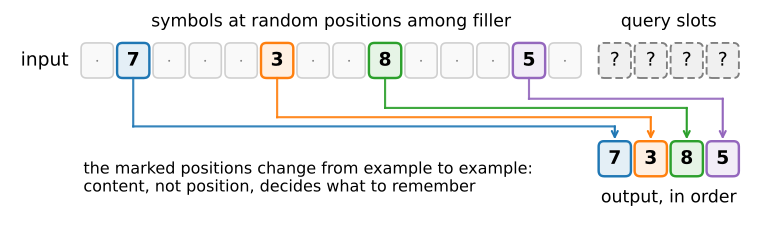
This toy is not idle. Its language-scale counterpart is associative recall: retrieving a value mentioned pages ago the next time its key appears (“Mrs. Watchett … later: Mrs. ___“). We have met the circuit that does this: it is the induction head of Section 10.6, which we built and watched form during training, and Arora et al. (2024) showed that a small synthetic recall benchmark of this kind predicts most of the language-modeling gap between attention and efficient recurrent models. A sequence model that cannot selectively copy has no business writing prose.
We generate the task synthetically: token \(0\) is filler, token \(1\) marks the query slots, and the symbols occupy ids \(2\) through \(9\). The targets are the eight-way symbol classes at the query positions.
def selective_copy(num_seqs, num_steps, num_marked, num_symbols, seed=42):
    """Sequences of filler (0) with num_marked symbols at random positions,
    followed by num_marked query slots (1); targets are the symbols."""
    rng = np.random.default_rng(seed)
    X = np.zeros((num_seqs, num_steps + num_marked), dtype=np.int64)
    X[:, num_steps:] = 1                          # Query slots
    Y = rng.integers(2, 2 + num_symbols, (num_seqs, num_marked))
    pos = np.argsort(rng.random((num_seqs, num_steps)), axis=1)
    pos = np.sort(pos[:, :num_marked], axis=1)    # Marked positions, in order
    np.put_along_axis(X, pos, Y, axis=1)
    return X, Y - 2                               # Classes 0..num_symbols-1

class SelectiveCopy(d2l.DataModule):
    def __init__(self, num_train=8192, num_val=1024, batch_size=128,
                 num_steps=256, num_marked=4, num_symbols=8):
        super().__init__()
        self.save_hyperparameters()
        X, Y = selective_copy(num_train + num_val, num_steps, num_marked,
                              num_symbols)
        self.X, self.Y = d2l.tensor(X), d2l.tensor(Y)

    def get_dataloader(self, train):
        idx = slice(0, self.num_train) if train else slice(self.num_train, None)
        return self.get_tensorloader([self.X, self.Y], train, idx)

copy_data = SelectiveCopy()
def selective_copy(num_seqs, num_steps, num_marked, num_symbols, seed=42):
"""Sequences of filler (0) with num_marked symbols at random positions,
followed by num_marked query slots (1); targets are the symbols."""
rng = np.random.default_rng(seed)
X = np.zeros((num_seqs, num_steps + num_marked), dtype=np.int64)
X[:, num_steps:] = 1 # Query slots
Y = rng.integers(2, 2 + num_symbols, (num_seqs, num_marked))
pos = np.argsort(rng.random((num_seqs, num_steps)), axis=1)
pos = np.sort(pos[:, :num_marked], axis=1) # Marked positions, in order
np.put_along_axis(X, pos, Y, axis=1)
return X, Y - 2 # Classes 0..num_symbols-1
class SelectiveCopy(d2l.DataModule):
def __init__(self, num_train=8192, num_val=1024, batch_size=128,
num_steps=256, num_marked=4, num_symbols=8):
super().__init__()
self.save_hyperparameters()
X, Y = selective_copy(num_train + num_val, num_steps, num_marked,
num_symbols)
self.X, self.Y = d2l.tensor(X), d2l.tensor(Y)
def get_dataloader(self, train):
idx = slice(0, self.num_train) if train else slice(self.num_train, None)
return self.get_tensorloader([self.X, self.Y], train, idx)
copy_data = SelectiveCopy()12.3.1.2 An LTI Baseline and a Gated One
The prosecution calls two witnesses from earlier sections. The LTI witness is the S4D stack exactly as we assembled it in Section 12.2.5: since that section saved both the layer and its residual block in the d2l library, two aliases suffice.
S4D, S4DBlock = d2l.S4D, d2l.S4DBlockS4D, S4DBlock = d2l.S4D, d2l.S4DBlockThe gated witness is the LSTM of Section 12.1, via the concise d2l.LSTM layer. Both plug into the same harness: embed the tokens, run the encoder, and classify each of the final query positions. As in Section 12.2.5 we train with Adam, the default of the training recipes in Section 7.6 and the right tool for parameters as differently scaled as log-decays and linear weights (the reasoning of Chapter 9); we clip gradients to norm 1, without which the LSTM destabilizes on these sequence lengths.
One implementation note: we embed tokens with a one-hot matrix product rather than an embedding lookup. A lookup’s gradient is a scatter-add, and on this task every batch pushes 33,000 colliding updates into a ten-row table, which XLA executes so slowly that it dominates the entire training step; as a dense product, both passes are ordinary matrix multiplications. Hold this thought: this section later argues that how a computation maps onto hardware can matter as much as what it computes.
class CopyModel(d2l.Classifier):
    """Read a token sequence; predict the symbols at the query slots."""
    def __init__(self, encoder, num_hiddens, vocab_size=10, num_marked=4,
                 num_symbols=8, lr=3e-3):
        super().__init__()
        self.save_hyperparameters()
        self.emb = nn.Embedding(vocab_size, num_hiddens)
        self.head = nn.LazyLinear(num_symbols)

    def forward(self, X):
        Y = self.encoder(self.emb(X.T))                 # (T, batch, hiddens)
        Y = Y[0] if isinstance(Y, tuple) else Y         # RNNs return a state
        return self.head(Y[-self.num_marked:]).movedim(0, 1)

    def configure_optimizers(self):
        return torch.optim.Adam(self.parameters(), lr=self.lr)
class CopyModel(d2l.Classifier):
"""Read a token sequence; predict the symbols at the query slots."""
def __init__(self, encoder, num_hiddens, vocab_size=10, num_marked=4,
num_symbols=8, num_features=None, lr=3e-3, rngs=None):
super().__init__()
self.save_hyperparameters(ignore=['encoder', 'rngs'])
rngs = nnx.Rngs(1) if rngs is None else rngs
num_features = num_hiddens if num_features is None else num_features
self.encoder = encoder
# Embed by one-hot matmul: on a table this tiny (ten rows), the
# scatter-add in an embedding lookup's gradient makes 33,000 colliding
# updates to ten rows and serializes the whole training step on GPU;
# as a dense product, forward and backward are ordinary matmuls
self.emb = nnx.Linear(vocab_size, num_hiddens, use_bias=False,
rngs=rngs)
self.head = nnx.Linear(num_features, num_symbols, rngs=rngs)
def forward(self, X):
E = self.emb(jax.nn.one_hot(X.T, self.vocab_size))
Y = self.encoder(E) # (T, batch, hiddens)
Y = Y[0] if isinstance(Y, tuple) else Y # RNNs return a state
return self.head(Y[-self.num_marked:]).swapaxes(0, 1)
def configure_optimizers(self):
return optax.adam(self.lr)We give each model the same budget and record its validation accuracy curve; copy_curves collects them, and a third contender will join in Section 12.3.3. The two encoders are sized to roughly 30,000 parameters each, the same pairing that Section 12.2.5 used for sequential image classification, where the S4D won.
copy_curves = {}

def train_copy(name, model, data, epochs=32):
    trainer = d2l.Trainer(max_epochs=epochs, gradient_clip_val=1, num_gpus=1)
    trainer.fit(model, data)
    pts = model.board.data['val_acc']
    copy_curves[name] = ([p.x for p in pts], [float(p.y) for p in pts])
    print(f'{name}: final validation accuracy {copy_curves[name][1][-1]:.3f}')

s4d = CopyModel(nn.Sequential(*[S4DBlock(48, 4) for _ in range(2)]),
                num_hiddens=48)
train_copy('S4D', s4d, copy_data)
S4D: final validation accuracy 0.597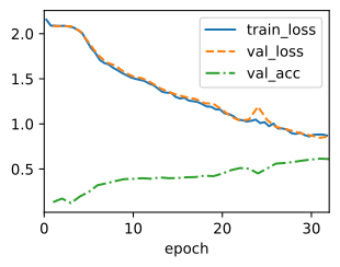
copy_curves = {}

def train_copy(name, model, data, epochs=32):
    trainer = d2l.Trainer(max_epochs=epochs, gradient_clip_val=1, num_gpus=1)
    trainer.fit(model, data)
    pts = model.board.data['val_acc']
    copy_curves[name] = ([p.x for p in pts], [float(p.y) for p in pts])
    print(f'{name}: final validation accuracy {copy_curves[name][1][-1]:.3f}')

s4d = CopyModel(nnx.Sequential(*[S4DBlock(48, 4) for _ in range(2)]),
                num_hiddens=48)
train_copy('S4D', s4d, copy_data)
S4D: final validation accuracy 0.631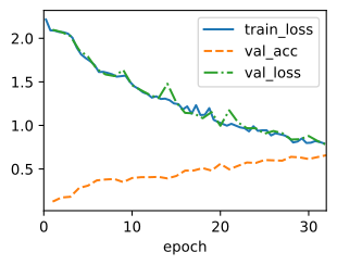
if tab.selected('pytorch'):
    lstm = CopyModel(d2l.LSTM(num_inputs=48, num_hiddens=64), num_hiddens=48)
if tab.selected('jax'):
    lstm = CopyModel(d2l.LSTM(num_inputs=48, num_hiddens=64), num_hiddens=48,
                     num_features=64)
train_copy('LSTM', lstm, copy_data)
LSTM: final validation accuracy 0.973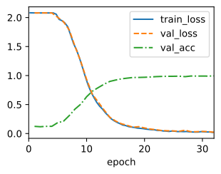
if tab.selected('pytorch'):
    lstm = CopyModel(d2l.LSTM(num_inputs=48, num_hiddens=64), num_hiddens=48)
if tab.selected('jax'):
    lstm = CopyModel(d2l.LSTM(num_inputs=48, num_hiddens=64), num_hiddens=48,
                     num_features=64)
train_copy('LSTM', lstm, copy_data)
LSTM: final validation accuracy 0.903
names = list(copy_curves)
d2l.plot([copy_curves[n][0] for n in names],
         [copy_curves[n][1] for n in names], 'epoch',
         'validation accuracy', legend=names, figsize=(5, 3))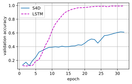
names = list(copy_curves)
d2l.plot([copy_curves[n][0] for n in names],
         [copy_curves[n][1] for n in names], 'epoch',
         'validation accuracy', legend=names, figsize=(5, 3))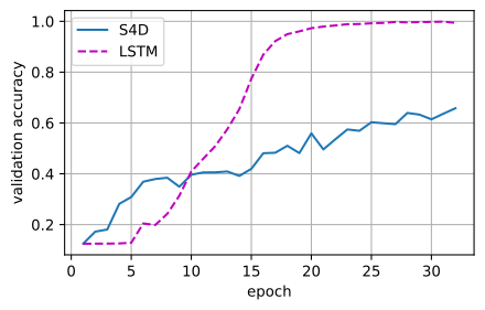
The curves separate the way the content-blindness argument predicts. Both models start at chance (one symbol in eight). The LSTM climbs toward a complete solution, and in our runs ends the budget well above 0.9, in some frameworks essentially perfect (how far it gets inside the budget depends on each framework’s initialization defaults, the same effect Section 12.2.5 dissected): its input and forget gates are functions of the data, so “store this, it is a symbol” is a computation it can learn, given enough epochs. The S4D improves slowly. Its pointwise nonlinear blocks can learn to suppress filler locally, which raises its accuracy well above chance, but the time-invariant state cannot cleanly align “the third symbol I saw” with “the third query slot” when the spacing between symbols changes from example to example, and it ends the same budget far from a solution. For this task, the older LSTM architecture is better suited to the required content-dependent updates. Its advantage is precisely the input dependence that Section 12.2 removed to enable a scan. The remaining question is whether input dependence can be restored without giving up parallel training.
12.3.2 Selective State Space Models
12.3.2.1 Input-Dependent Dynamics
Recall from Section 12.2.3.1 where the S4D’s dynamics come from: a continuous system \((\mathbf{A}, \mathbf{B}, \mathbf{C})\) and a step size \(\Delta\), discretized by the zero-order hold into per-step coefficients. The downstream construction remains fixed; the selective state space model of Gu and Dao (2023) changes one design principle: the SSM’s parameters become functions of the input. Three coupled projections realize that principle. The step size, the input matrix, and the read-out are no longer constants but functions of the current input \(\mathbf{u}_t \in \mathbb{R}^H\):
\[ \boldsymbol{\Delta}_t = \textrm{softplus}(\mathbf{u}_t \mathbf{W}_{\Delta} + \mathbf{b}_{\Delta}), \qquad \mathbf{B}_t = \mathbf{u}_t \mathbf{W}_{\textrm{B}}, \qquad \mathbf{C}_t = \mathbf{u}_t \mathbf{W}_{\textrm{C}}, \tag{12.3.1}\]
with \(\boldsymbol{\Delta}_t \in \mathbb{R}^H\) holding one step size per channel (softplus keeps it positive) and \(\mathbf{B}_t, \mathbf{C}_t \in \mathbb{R}^N\) shared across channels. The state matrix \(\mathbf{A} = \textrm{diag}(a_1, \ldots, a_N)\) keeps its fixed S4D parameterization; it sets the menu of decay rates, while \(\boldsymbol{\Delta}_t\) decides, per token, how far along that menu to step. Discretizing exactly as before, channel \(h\) of the layer now obeys
\[ \mathbf{x}_t = e^{\Delta_{t,h} \mathbf{a}} \odot \mathbf{x}_{t-1} + \Delta_{t,h}\, u_{t,h}\, \mathbf{B}_t, \qquad y_{t,h} = \mathbf{C}_t^\top \mathbf{x}_t + d_h\, u_{t,h}, \tag{12.3.2}\]
where \(\mathbf{x}_t \in \mathbb{R}^N\) is that channel’s state. (Mamba simplifies the zero-order hold on the input path to the first-order rule \(\bar{\mathbf{B}}_t = \Delta_{t,h} \mathbf{B}_t\); the exponential on the state path, which controls stability, is kept exact.)
The correspondence in Section 12.2.3.1 gives a direct interpretation of an input-dependent \(\Delta\). There, a small \(\Delta\) froze the state and ignored the input; a large \(\Delta\) flushed the state and admitted the input. Make \(\Delta\) a function of \(\mathbf{u}_t\) and the model can choose per token: filler should produce \(\Delta_t \approx 0\) (the state changes little and the input contributes almost nothing), while a marked symbol should produce a large \(\Delta_t\) (reset toward the new content). That is a forget gate and an input gate, fused into one scalar acting on a linear state. The same gating mechanism has arisen from three requirements: controlled memory updates (Section 12.1), numerical integration (Section 12.2.3.1), and content-dependent selection in a linear recurrence. \(\mathbf{B}_t\) and \(\mathbf{C}_t\) similarly control where input enters the state and which state coordinates are read out; an exercise asks how much they add over selectivity in \(\Delta\) alone.
12.3.2.2 Parallel Evaluation with Selectivity
With time-varying coefficients, the model is no longer LTI and the convolutional view of Section 12.2.3.2 no longer applies. There is no fixed kernel \(\bar{\mathbf{K}}\) to materialize and no FFT shortcut; of the three views in Figure 12.2.2, only the recurrence survives. This is why we built the scan rather than the FFT in Section 12.2. The recurrence Equation 12.3.2 is still an affine map of the state, just with per-step coefficients, and the associative combine Equation 12.2.4 never assumed those coefficients were constant. The same associative_scan evaluates the selective recurrence in the same logarithmic depth, now called with tensors whose leading axis varies per step. We verify this equivalence by comparing a sequential loop with time-varying decays against the scan.
num_steps, num_states = 100, 4
a_t = torch.rand(num_steps, num_states)      # Per-step decays in (0, 1)
b_t = torch.randn(num_steps, num_states)     # Per-step inputs
h, ys = torch.zeros(num_states), []
for t in range(num_steps):
    h = a_t[t] * h + b_t[t]
    ys.append(h)
err = (associative_scan(a_t, b_t) - torch.stack(ys)).abs().max()
print(f'time-varying scan vs loop: {float(err):.2e}')
time-varying scan vs loop: 3.58e-07num_steps, num_states = 100, 4
key1, key2 = jax.random.split(d2l.get_key())
a_t = jax.random.uniform(key1, (num_steps, num_states)) # Decays in (0, 1)
b_t = jax.random.normal(key2, (num_steps, num_states)) # Per-step inputs
h, ys = jnp.zeros(num_states), []
for t in range(num_steps):
h = a_t[t] * h + b_t[t]
ys.append(h)
err = jnp.abs(associative_scan(a_t, b_t) - jnp.stack(ys)).max()
print(f'time-varying scan vs loop: {float(err):.2e}')time-varying scan vs loop: 4.77e-07The layer below packages Equation 12.3.1 and Equation 12.3.2. Next to the S4D class it differs in three places: \(\Delta\), \(\mathbf{B}\), \(\mathbf{C}\) are computed from u by small linear heads rather than stored as parameters; the \(\Delta\) head is factored through rank \(H/16\) (Mamba’s dt_rank), which keeps its parameter count negligible; and its bias is initialized so that \(\textrm{softplus}\) of it reproduces the log-uniform step sizes of Section 12.2.5. Only the initial decay timescales carry over from the S4D, though: \(\mathbf{B}_t\) and \(\mathbf{C}_t\) come out of randomly initialized heads, so the layer is input-dependent from its first forward pass rather than starting as an LTI system. The scan call is unchanged, except that the decay tensor now genuinely spans (num_steps, batch, H, N) instead of broadcasting one value.
class SelectiveSSM(nn.Module):
    """A diagonal SSM whose step size, input matrix, and read-out are
    functions of the input (Gu & Dao, 2023)."""
    def __init__(self, num_hiddens, num_states=4, dt_min=0.001, dt_max=0.1):
        super().__init__()
        H, N, R = num_hiddens, num_states, max(2, num_hiddens // 16)
        self.log_a = nn.Parameter(
            torch.log(torch.arange(1., N + 1)).repeat(H, 1))
        self.W_dt = nn.Sequential(nn.Linear(H, R), nn.Linear(R, H, bias=False))
        dt = torch.exp(torch.rand(H) * math.log(dt_max / dt_min)
                       + math.log(dt_min))
        self.b_dt = nn.Parameter(dt + torch.log(-torch.expm1(-dt)))
        self.W_B = nn.Linear(H, N, bias=False)
        self.W_C = nn.Linear(H, N, bias=False)
        self.D = nn.Parameter(torch.ones(H))

    def forward(self, u):                    # (num_steps, batch, num_hiddens)
        a = -torch.exp(self.log_a)                    # (H, N), Re(a) < 0
        dt = F.softplus(self.W_dt(u) + self.b_dt)     # (T, batch, H)
        B, C = self.W_B(u), self.W_C(u)               # (T, batch, N)
        a_bar = torch.exp(dt.unsqueeze(-1) * a)       # (T, batch, H, N)
        b_bar = (dt * u).unsqueeze(-1) * B.unsqueeze(-2)
        x = associative_scan(a_bar, b_bar)
        return (x * C.unsqueeze(-2)).sum(-1) + self.D * u
class SelectiveSSM(nnx.Module):
"""A diagonal SSM whose step size, input matrix, and read-out are
functions of the input (Gu & Dao, 2023)."""
def __init__(self, num_hiddens, num_states=4, dt_min=0.001, dt_max=0.1,
rngs=None):
rngs = nnx.Rngs(0) if rngs is None else rngs
H, N, R = num_hiddens, num_states, max(2, num_hiddens // 16)
self.log_a = nnx.Param(jnp.tile(jnp.log(jnp.arange(1., N + 1)),
(H, 1)))
self.W_dt = nnx.Sequential(
nnx.Linear(H, R, rngs=rngs),
nnx.Linear(R, H, use_bias=False, rngs=rngs))
dt = jnp.exp(rngs.params.uniform((H,)) * math.log(dt_max / dt_min)
+ math.log(dt_min))
self.b_dt = nnx.Param(dt + jnp.log(-jnp.expm1(-dt)))
self.W_B = nnx.Linear(H, N, use_bias=False, rngs=rngs)
self.W_C = nnx.Linear(H, N, use_bias=False, rngs=rngs)
self.D = nnx.Param(jnp.ones(H))
def __call__(self, u): # (num_steps, batch, num_hiddens)
a = -jnp.exp(self.log_a[...]) # (H, N), Re(a) < 0
dt = jax.nn.softplus(self.W_dt(u) + self.b_dt) # (T, batch, H)
B, C = self.W_B(u), self.W_C(u) # (T, batch, N)
a_bar = jnp.exp(dt[..., None] * a) # (T, batch, H, N)
b_bar = (dt * u)[..., None] * B[..., None, :]
x = associative_scan(a_bar, b_bar)
return (x * C[..., None, :]).sum(-1) + self.D * uOne prose remark on engineering, because it explains why this architecture arrived in 2023 rather than 2020. Our implementation materializes the (num_steps, batch, H, N) coefficient tensors in GPU memory, which is fine at textbook scale and ruinous at model scale: the computation is trivially cheap per element, so its speed is set entirely by memory traffic. The Mamba authors’ kernel never materializes those tensors. It fuses discretization, scan, and read-out into a single pass that keeps intermediates in fast on-chip memory, and during backpropagation recomputes them from the small inputs instead of storing them, trading a little arithmetic for a lot of bandwidth, the same store-versus-recompute trade we met in Section 8.6. None of this changes what is computed. It changed whether the architecture was worth computing, and it is half the reason the paper’s title contains the word “hardware-aware”.
12.3.3 The Mamba Block
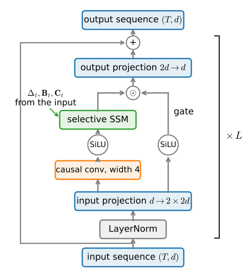
The selective SSM mixes information across time. Like the S4D it needs a scaffold around it that mixes channels and supplies nonlinearity, and Mamba’s block, Figure 12.3.2, differs instructively from the S4D block of Figure 12.2.4. Instead of alternating a sequence layer with a separate gated MLP, Mamba fuses the two: one linear projection widens the input from \(d\) to an expanded \(2d\) and forks it into two branches. The main branch is convolved with a short causal convolution (width 4; a cheap way to let each token see a few immediate predecessors before deciding its dynamics), passed through a SiLU activation, and fed to the selective SSM. The other branch, after its own SiLU, multiplies the SSM’s output elementwise, one final gate, echoing Section 12.1 yet again, so that even the read-out is content-controlled. A linear projection maps the expanded width back to \(d\), and the whole thing sits inside the usual pre-norm residual.
The comparison with the transformer block of Section 11.1 is worth making precisely. That block divides its labor: an attention sub-block mixes information across positions, then an MLP sub-block (with its own residual and normalization) mixes across channels, and the two alternate through the stack. Mamba fuses the same two jobs into one unit: the selective SSM is the sequence mixer, the expanded gated projections around it are the channel mixer, and a Mamba language model is this single homogeneous block stacked \(L\) times where a transformer alternates two. The deeper question is exactly where this chapter is headed: whether the mixers themselves are secretly the same operation.
With SelectiveSSM in hand the block is a dozen lines, and a language model is the block stacked plus the embedding and head that d2l.RNNLM of Section 8.5 already provides. The stack exposes the (inputs, state) calling convention of our recurrent cells, so it drops into the same scaffold as every other model in this chapter; like the S4D, it trains with Adam. All three classes go into the d2l library: the chapter’s closing section builds its hybrid stacks out of them.
class MambaBlock(nn.Module):
    """Conv + SiLU + selective SSM, gated, inside a pre-norm residual."""
    def __init__(self, num_hiddens, num_states=4, expand=2, conv_width=4,
                 dropout=0):
        super().__init__()
        d = expand * num_hiddens
        self.ln = nn.LayerNorm(num_hiddens)
        self.W_in = nn.Linear(num_hiddens, 2 * d)
        self.conv = nn.Conv1d(d, d, conv_width, groups=d,
                              padding=conv_width - 1)
        self.ssm = SelectiveSSM(d, num_states)
        self.W_out = nn.Linear(d, num_hiddens)
        self.drop = nn.Dropout(dropout)

    def forward(self, X):                    # (num_steps, batch, num_hiddens)
        u, gate = self.W_in(self.ln(X)).chunk(2, -1)
        u = self.conv(u.permute(1, 2, 0))[..., :X.shape[0]]  # Causal: trim
        y = self.ssm(F.silu(u.permute(2, 0, 1)))
        return X + self.drop(self.W_out(y * F.silu(gate)))

class Mamba(d2l.Module):
    """A stack of Mamba blocks with the recurrent-cell interface."""
    def __init__(self, num_inputs, num_blocks=2, num_states=4, dropout=0):
        super().__init__()
        self.save_hyperparameters()
        self.num_hiddens = num_inputs                 # Output width, for heads
        self.blocks = nn.Sequential(*[
            MambaBlock(num_inputs, num_states, dropout=dropout)
            for _ in range(num_blocks)])
        self.ln = nn.LayerNorm(num_inputs)

    def forward(self, X, state=None):
        return self.ln(self.blocks(X)), None
class MambaBlock(nnx.Module):
"""Conv + SiLU + selective SSM, gated, inside a pre-norm residual."""
def __init__(self, num_hiddens, num_states=4, expand=2, conv_width=4,
dropout=0, rngs=None):
rngs = nnx.Rngs(0) if rngs is None else rngs
d = expand * num_hiddens
self.ln = nnx.LayerNorm(num_hiddens, rngs=rngs)
self.W_in = nnx.Linear(num_hiddens, 2 * d, rngs=rngs)
self.conv = nnx.Conv(d, d, kernel_size=(conv_width,),
feature_group_count=d, padding='CAUSAL',
rngs=rngs)
self.ssm = SelectiveSSM(d, num_states, rngs=rngs)
self.W_out = nnx.Linear(d, num_hiddens, rngs=rngs)
self.drop = nnx.Dropout(dropout, rngs=rngs)
def __call__(self, X): # (num_steps, batch, num_hiddens)
u, gate = jnp.split(self.W_in(self.ln(X)), 2, axis=-1)
u = jnp.swapaxes(self.conv(jnp.swapaxes(u, 0, 1)), 0, 1)
y = self.ssm(jax.nn.silu(u))
return X + self.drop(self.W_out(y * jax.nn.silu(gate)))
class Mamba(nnx.Module):
"""A stack of Mamba blocks with the recurrent-cell interface."""
def __init__(self, num_inputs, num_blocks=2, num_states=4, dropout=0,
rngs=None):
rngs = nnx.Rngs(0) if rngs is None else rngs
self.num_inputs = self.num_hiddens = num_inputs
self.blocks = nnx.Sequential(*[
MambaBlock(num_inputs, num_states, dropout=dropout, rngs=rngs)
for _ in range(num_blocks)])
self.ln = nnx.LayerNorm(num_inputs, rngs=rngs)
def __call__(self, X, state=None):
return self.ln(self.blocks(X)), NoneWhat we have just assembled is a pedagogical Mamba-style block, not a reproduction of the paper’s implementation. Table 12.3.1 records what carries over and what was cut down, so that the measurements below are read at the right resolution.
| kept from Mamba | simplified here | effect |
|---|---|---|
| the selective mechanism Equation 12.3.1–Equation 12.3.2: \(\Delta, \mathbf{B}, \mathbf{C}\) from the input, exact exponential state decay, S4D-style \(\mathbf{A}\) and \(\Delta\)-bias initialization, the conv–SiLU–gate block layout | nothing | the mechanism the experiments probe is the paper’s |
| the scan’s mathematics: the same affine combine, the same logarithmic depth | the fused kernel becomes a generic associative_scan that materializes the \((T, \textrm{batch}, H, N)\) coefficient tensors |
identical outputs; memory traffic sets the wall clock, the slow s/epoch column below |
| the block interface: width expansion, gating, pre-norm residual | textbook scale (\(N = 4\) states, two blocks), LayerNorm in place of RMSNorm, added dropout | small enough to train in a notebook; the results are illustrations at this scale, not scaling claims |
12.3.3.1 Comparing Recurrent Models
This chapter proposed three answers to its opening question of what a hidden state should remember: gate it (the LSTM), linearize it (the minGRU and the SSMs), select it (Mamba). Time to put all three on one scoreboard. The task is the language-modeling recipe used throughout, The Time Machine under the 1,024-token BPE tokenizer of Section 8.5, 50,000 windows of 32 tokens, ten epochs, gradients clipped to norm 1. Alongside perplexity we report bits per byte (all three models share one tokenizer, but bpb keeps the scoreboard comparable with the character-level models of Chapter 8), parameter counts, and wall clock per epoch. The tokens-to-bytes conversion decodes the full validation target stream, so bpb is normalized over exactly the tokens that the validation perplexity averages.
data = d2l.TimeMachine(batch_size=1024, num_steps=32,
                       num_train=50000, num_val=5000)
ids = d2l.numpy(data.Y[data.num_train:data.num_train + data.num_val]
                ).reshape(-1).tolist()               # Full val target stream
bytes_per_token = len(data.tokenizer.decode(ids).encode('utf-8')) / len(ids)
data = d2l.TimeMachine(batch_size=1024, num_steps=32,
num_train=50000, num_val=5000)
ids = d2l.numpy(data.Y[data.num_train:data.num_train + data.num_val]
).reshape(-1).tolist() # Full val target stream
bytes_per_token = len(data.tokenizer.decode(ids).encode('utf-8')) / len(ids)results = {}
def benchmark(name, model, epochs=10):
trainer = d2l.Trainer(max_epochs=epochs, gradient_clip_val=1, num_gpus=1)
model.board.yscale = 'log'
start = time.time()
trainer.fit(model, data)
secs = (time.time() - start) / epochs
ppl = float(model.board.data['val_ppl'][-1].y)
params = sum(p.numel() for p in model.parameters() if p.requires_grad)
results[name] = (ppl, math.log2(ppl) / bytes_per_token, params, secs)results = {}
def val_ppl(model):
model = nnx.view(model, deterministic=True, use_running_average=True,
raise_if_not_found=False) # Dropout off for evaluation
total_loss = num_tokens = 0
for X_val, y_val in data.val_dataloader():
losses = model.loss(model(X_val), y_val, averaged=False)
total_loss += float(losses.sum())
num_tokens += losses.size
return math.exp(total_loss / num_tokens)
def benchmark(name, model, epochs=10):
trainer = d2l.Trainer(max_epochs=epochs, gradient_clip_val=1, num_gpus=1)
model.board.yscale = 'log'
start = time.time()
trainer.fit(model, data)
secs = (time.time() - start) / epochs
params = sum(p.size for p in
jax.tree.leaves(nnx.state(model, nnx.Param)))
results[name] = (val_ppl(model), math.log2(val_ppl(model))
/ bytes_per_token, params, secs)The first two answers train with the exact recipes of their home sections: the LSTM of Section 12.1 and the minGRU of Section 12.2.1 (restated below).
lstm_lm = d2l.RNNLM(d2l.LSTM(num_inputs=64, num_hiddens=128),
                    vocab_size=len(data.vocab), lr=4)
benchmark('LSTM', lstm_lm)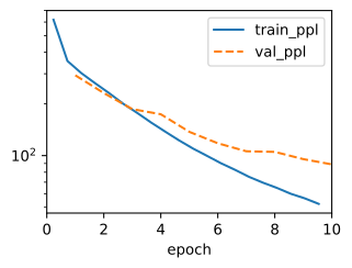
lstm_lm = d2l.RNNLM(d2l.LSTM(num_inputs=64, num_hiddens=128),
                    vocab_size=len(data.vocab), lr=4)
benchmark('LSTM', lstm_lm)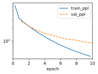
class MinGRU(d2l.Module):
    """The minimal GRU of the previous section."""
    def __init__(self, num_inputs, num_hiddens):
        super().__init__()
        self.save_hyperparameters()
        self.W_xz = nn.Linear(num_inputs, num_hiddens)
        self.W_xh = nn.Linear(num_inputs, num_hiddens)

    def forward(self, inputs, H=None):
        Z = torch.sigmoid(self.W_xz(inputs))     # (num_steps, batch, hiddens)
        H_tilde = torch.tanh(self.W_xh(inputs))
        a, b = 1 - Z, Z * H_tilde
        if H is not None:  # Fold the carried-in state into the first step
            b = torch.cat([b[:1] + a[:1] * H, b[1:]])
        outputs = associative_scan(a, b)
        return outputs, outputs[-1]

mingru_lm = d2l.RNNLM(MinGRU(num_inputs=64, num_hiddens=128),
                      vocab_size=len(data.vocab), lr=4)
benchmark('minGRU', mingru_lm)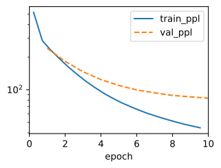
class MinGRU(nnx.Module):
    """The minimal GRU of the previous section."""
    def __init__(self, num_inputs, num_hiddens, rngs=None):
        rngs = nnx.Rngs(0) if rngs is None else rngs
        self.num_inputs, self.num_hiddens = num_inputs, num_hiddens
        self.W_xz = nnx.Linear(num_inputs, num_hiddens, rngs=rngs)
        self.W_xh = nnx.Linear(num_inputs, num_hiddens, rngs=rngs)

    def __call__(self, inputs, H=None):
        Z = jax.nn.sigmoid(self.W_xz(inputs))    # (num_steps, batch, hiddens)
        H_tilde = jnp.tanh(self.W_xh(inputs))
        a, b = 1 - Z, Z * H_tilde
        if H is not None:  # Fold the carried-in state into the first step
            b = jnp.concatenate([b[:1] + a[:1] * H, b[1:]])
        outputs = associative_scan(a, b)
        return outputs, outputs[-1]

mingru_lm = d2l.RNNLM(MinGRU(num_inputs=64, num_hiddens=128),
                      vocab_size=len(data.vocab), lr=4)
benchmark('minGRU', mingru_lm)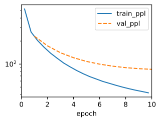
The third answer stacks two Mamba blocks at model width 128. Since d2l.RNNLM supplies embedding and head around any module with the (inputs, state) interface, only the optimizer needs overriding. One adjustment is needed, and it is a compliment in disguise: trained like the baselines, this model overfits. Its validation perplexity bottoms out within a few epochs and then climbs while training perplexity keeps falling toward single digits, which no gated model in this chapter comes close to doing; a selective state is, among other things, an excellent memorization device, and our corpus is one short novel. So Mamba, alone in this chapter, gets the standard medicine of Section 4.6, dropout on each block’s residual branch, plus a gentler learning rate.
class MambaLM(d2l.RNNLM):
    def configure_optimizers(self):
        return torch.optim.Adam(self.parameters(), lr=self.lr)

mamba_lm = MambaLM(Mamba(num_inputs=128, dropout=0.3),
                   vocab_size=len(data.vocab), lr=3e-4)
benchmark('Mamba', mamba_lm)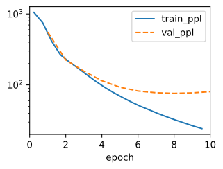
class MambaLM(d2l.RNNLM):
    def configure_optimizers(self):
        return optax.adam(self.lr)

mamba_lm = MambaLM(Mamba(num_inputs=128, dropout=0.3),
                   vocab_size=len(data.vocab), lr=3e-4)
benchmark('Mamba', mamba_lm)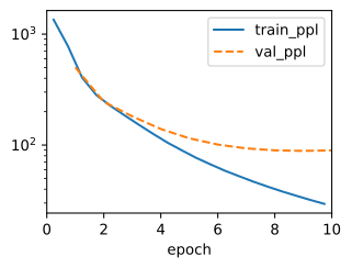
print(f'{"model":>7} {"val ppl":>8} {"bpb":>6} {"params":>9} {"s/epoch":>8}')
for name, (ppl, bpb, params, secs) in results.items():
    print(f'{name:>7} {ppl:>8.1f} {bpb:>6.2f} {params:>9,} {secs:>8.1f}')
model val ppl bpb params s/epoch
LSTM 91.7 2.35 297,539 0.9
minGRU 85.2 2.31 214,851 1.0
Mamba 75.0 2.24 488,739 6.3print(f'{"model":>7} {"val ppl":>8} {"bpb":>6} {"params":>9} {"s/epoch":>8}')
for name, (ppl, bpb, params, secs) in results.items():
print(f'{name:>7} {ppl:>8.1f} {bpb:>6.2f} {params:>9,} {secs:>8.1f}') model val ppl bpb params s/epoch
LSTM 91.4 2.34 297,027 1.7
minGRU 85.7 2.31 214,851 1.0
Mamba 88.6 2.33 488,739 2.8Numbers first, then caveats. In every framework we run, Mamba lands below the LSTM, by a few points of perplexity in some reruns and by tens in others, at a parameter count larger than the LSTM’s (most of the extra sits in the block’s expanded projections) and a slower epoch, our scan being the teaching-grade version of the fused kernel discussed above. In most runs it posts the best number of the chapter outright, though in some the minGRU, at fewer than half the parameters, stays within a few points or even edges it out: at this scale, framework initialization defaults and optimizer choices move the scoreboard by amounts comparable to the architectural gap. The caveats cut both ways: Mamba trains with Adam and dropout while the gated baselines keep their sections’ plain SGD recipe, and at this corpus size a stronger model mostly buys sharper memorization of Wells’s prose. This scoreboard says the selective architecture can be trained to better held-out prediction at comparable scale, not that it dominates pound for pound; at research scale the corresponding claim is the Mamba paper’s central result, matching transformers at small model sizes.
12.3.3.2 Stepping the Selective Model
Before sampling, we verify that recurrent stepping matches the parallel form. Section 12.2.6 stepped the LTI model one token at a time; does the trick survive selectivity? It does, and for a reason worth noticing: Equation 12.3.1 computes \(\boldsymbol{\Delta}_t,
\mathbf{B}_t, \mathbf{C}_t\) from the current input alone, so a single token is all the step needs to build its own coefficients before applying the same recurrence as before. The one genuinely new piece of state sits outside the SSM: the block’s causal convolution looks at the last conv_width inputs, so the step must carry a rolling buffer of the four most recent values alongside the \((H, N)\) state. This pair, conv buffer plus SSM state, is exactly what production Mamba implementations cache during decoding; it is the entire inference-time memory of a layer, a few kilobytes where a transformer layer’s KV cache grows by Equation 11.3.1 with every token generated (Section 11.3).
@d2l.add_to_class(SelectiveSSM)
def step(self, u, x=None):
    """Advance one token: u is (batch, H); x is the (batch, H, N) state."""
    a = -torch.exp(self.log_a)
    dt = F.softplus(self.W_dt(u) + self.b_dt)         # (batch, H)
    B, C = self.W_B(u), self.W_C(u)                   # (batch, N)
    a_bar = torch.exp(dt.unsqueeze(-1) * a)           # (batch, H, N)
    b_bar = (dt * u).unsqueeze(-1) * B.unsqueeze(-2)
    x = b_bar if x is None else a_bar * x + b_bar
    return (x * C.unsqueeze(-2)).sum(-1) + self.D * u, x

@d2l.add_to_class(MambaBlock)
def step(self, X, state=None):
    """Advance one token, carrying (conv buffer, SSM state)."""
    u, gate = self.W_in(self.ln(X)).chunk(2, -1)
    if state is None:
        state = (u.new_zeros(*u.shape, self.conv.kernel_size[0]), None)
    buf, x = state
    buf = torch.cat([buf[..., 1:], u.unsqueeze(-1)], -1)  # Roll the window
    u = (buf * self.conv.weight[:, 0]).sum(-1) + self.conv.bias
    y, x = self.ssm.step(F.silu(u), x)
    return X + self.drop(self.W_out(y * F.silu(gate))), (buf, x)

@d2l.add_to_class(Mamba)
def step(self, X, state=None):
    """Advance the stack one token: X is (batch, d); one state per block."""
    state = [None] * len(self.blocks) if state is None else list(state)
    for i, blk in enumerate(self.blocks):
        X, state[i] = blk.step(X, state[i])
return self.ln(X), state@d2l.add_to_class(SelectiveSSM)
def step(self, u, x=None):
"""Advance one token: u is (batch, H); x is the (batch, H, N) state."""
a = -jnp.exp(self.log_a[...])
dt = jax.nn.softplus(self.W_dt(u) + self.b_dt) # (batch, H)
B, C = self.W_B(u), self.W_C(u) # (batch, N)
a_bar = jnp.exp(dt[..., None] * a) # (batch, H, N)
b_bar = (dt * u)[..., None] * B[..., None, :]
x = b_bar if x is None else a_bar * x + b_bar
return (x * C[..., None, :]).sum(-1) + self.D * u, x
@d2l.add_to_class(MambaBlock)
def step(self, X, state=None):
"""Advance one token, carrying (conv buffer, SSM state)."""
u, gate = jnp.split(self.W_in(self.ln(X)), 2, axis=-1)
if state is None:
state = (jnp.zeros((u.shape[0], self.conv.kernel_size[0],
u.shape[-1])), None)
buf, x = state
buf = jnp.concatenate([buf[:, 1:], u[:, None]], 1) # Roll the window
u = (buf * self.conv.kernel[:, 0]).sum(1) + self.conv.bias
y, x = self.ssm.step(jax.nn.silu(u), x)
return X + self.drop(self.W_out(y * jax.nn.silu(gate))), (buf, x)
@d2l.add_to_class(Mamba)
def step(self, X, state=None):
"""Advance the stack one token: X is (batch, d); one state per block."""
state = ([None] * len(self.blocks.layers) if state is None
else list(state))
for i, blk in enumerate(self.blocks.layers):
X, state[i] = blk.step(X, state[i])
return self.ln(X), stateAs in Section 12.2.6, the check that matters runs on the trained model: we push a batch of validation windows through the capstone language model with the scan, then again token by token with step, and assert that the logits agree, relative to their scale, far more tightly than float32 rounding is obliged to deliver. (Dropout must be off, or the two passes would disagree by design.)
mamba_lm.eval()                                  # Dropout off
X = data.X[data.num_train:data.num_train + 8].to(d2l.try_gpu())
with torch.no_grad():
    logits_scan = mamba_lm(X)                    # (batch, T, vocab)
    state, cols = None, []
    for t in range(X.shape[1]):                  # One token at a time
        emb = mamba_lm.emb(X[:, t].unsqueeze(0)) # (1, batch, d)
        y, state = mamba_lm.rnn.step(emb[0], state)
        cols.append(mamba_lm.linear(y))
    logits_step = torch.stack(cols, 1)
err = float((logits_step - logits_scan).abs().max())
scale = float(logits_scan.abs().max())
print(f'stepped vs scanned logits: deviation {err:.2e}, '
      f'relative {err / scale:.2e}')
assert err < 1e-3 * scale
stepped vs scanned logits: deviation 5.72e-06, relative 5.30e-07eval_lm = nnx.view(mamba_lm, deterministic=True, use_running_average=True,
raise_if_not_found=False) # Dropout off
X = jnp.asarray(data.X[data.num_train:data.num_train + 8])
with jax.default_matmul_precision('float32'): # TF32 off, as before
logits_scan = eval_lm(X) # (batch, T, vocab)
state, cols = None, []
for t in range(X.shape[1]): # One token at a time
emb = eval_lm.emb(X[:, t][None]) # (1, batch, d)
y, state = eval_lm.rnn.step(emb[0], state)
cols.append(eval_lm.linear(y))
logits_step = jnp.stack(cols, 1)
err = float(jnp.abs(logits_step - logits_scan).max())
scale = float(jnp.abs(logits_scan).max())
print(f'stepped vs scanned logits: deviation {err:.2e}, '
f'relative {err / scale:.2e}')
assert err < 1e-3 * scalestepped vs scanned logits: deviation 4.29e-06, relative 4.02e-07We also evaluate the language models through generation, following Section 8.7. We sample each model with the same prefix, temperature, and min-\(p\) filter, using the d2l.generate helper built there. For the gated baselines we keep that section’s harness, which re-runs the growing prefix at every token; for Mamba we use recurrent decoding. d2l.generate hands our callback the full token list each call, so the closure below keeps (state, seen) and feeds only the unseen suffix through step: the first call plays the prompt into the state and every later call advances one token, the same prefill/decode split that Section 11.3 built for the transformer, except that here the “cache” never grows. Generation cost falls from quadratic in the output length to linear.
def step_fn(model):
    def step(ids):  # Token ids in, numpy logits for the next token out
        with torch.no_grad():
            logits = model(d2l.tensor([ids], device=d2l.try_gpu()))
        return d2l.numpy(logits)[0, -1]
    return step

def stepped_fn(model):
    state, seen = None, 0
    def step(ids):  # Consume only the tokens the state has not absorbed
        nonlocal state, seen
        with torch.no_grad():
            for i in ids[seen:]:
                emb = model.emb(d2l.tensor([[i]], device=d2l.try_gpu()))
                y, state = model.rnn.step(emb[0], state)
            seen = len(ids)
            return d2l.numpy(model.linear(y))[0]
    return step

prefix = data.tokenizer.encode('the time traveller')
for name, model, fn in [('LSTM', lstm_lm, step_fn),
                        ('minGRU', mingru_lm, step_fn),
                        ('Mamba', mamba_lm, stepped_fn)]:
    out = d2l.generate(fn(model), prefix, 25, strategy='sample',
                       temperature=1.0, min_p=0.1,
                       rng=np.random.default_rng(0))
    d2l.print_wrapped(f'{name:>7}: {data.tokenizer.decode(out)!r}')
LSTM: 'the time traveller. I\nfindted that is stumbrcepts, but the\ngrew
pretal'
minGRU: 'the time traveller, and the\nmere came in the Dimensions. It was I
fancied to\nto the'
Mamba: 'the time traveller was examinionoth of\nhast. Some way, I was in
the sensible of d'def step_fn(model):
model = nnx.view(model, deterministic=True, use_running_average=True,
raise_if_not_found=False) # Dropout off for sampling
def step(ids): # Token ids in, numpy logits for the next token out
return d2l.numpy(model(d2l.tensor([ids])))[0, -1]
return step
def stepped_fn(model):
model = nnx.view(model, deterministic=True, use_running_average=True,
raise_if_not_found=False) # Dropout off for sampling
state, seen = None, 0
def step(ids): # Consume only the tokens the state has not absorbed
nonlocal state, seen
for i in ids[seen:]:
emb = model.emb(jnp.array([[i]]))
y, state = model.rnn.step(emb[0], state)
seen = len(ids)
return d2l.numpy(model.linear(y))[0]
return step
prefix = data.tokenizer.encode('the time traveller')
for name, model, fn in [('LSTM', lstm_lm, step_fn),
('minGRU', mingru_lm, step_fn),
('Mamba', mamba_lm, stepped_fn)]:
out = d2l.generate(fn(model), prefix, 25, strategy='sample',
temperature=1.0, min_p=0.1,
rng=np.random.default_rng(0))
d2l.print_wrapped(f'{name:>7}: {data.tokenizer.decode(out)!r}') LSTM: 'the time traveller. I had\nconanted to fue. And the same\nwas
circumstant, as'
minGRU: "the time traveller,\nand a moment\nI dw up down the three-
down.\n\n'I must have\n"
Mamba: 'the time traveller, I was not know. One of a\nmind, but the
weather-world people as\nthis'12.3.3.3 Selective Copying, Revisited
The language-model comparison evaluates end-to-end quality; the opening copying task isolates content-dependent selection. We run the Mamba stack on the selective copying task that the S4D could not solve, at the same parameter budget as before, and replot all three curves together.
mamba_copy = CopyModel(nn.Sequential(*[MambaBlock(48, 4) for _ in range(2)]),
                       num_hiddens=48)
train_copy('Mamba', mamba_copy, copy_data)
Mamba: final validation accuracy 1.000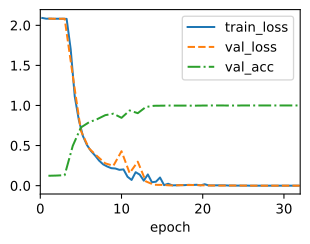
mamba_copy = CopyModel(
    nnx.Sequential(*[MambaBlock(48, 4) for _ in range(2)]), num_hiddens=48)
train_copy('Mamba', mamba_copy, copy_data)
Mamba: final validation accuracy 1.000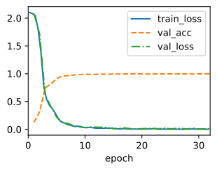
names = list(copy_curves)
d2l.plot([copy_curves[n][0] for n in names],
         [copy_curves[n][1] for n in names], 'epoch',
         'validation accuracy', legend=names, figsize=(5, 3))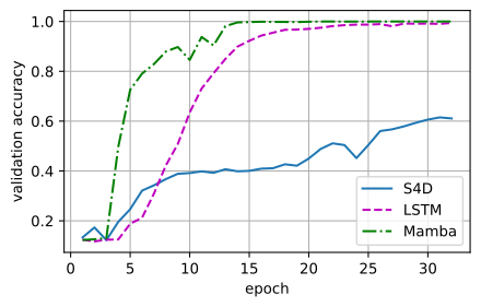
names = list(copy_curves)
d2l.plot([copy_curves[n][0] for n in names],
         [copy_curves[n][1] for n in names], 'epoch',
         'validation accuracy', legend=names, figsize=(5, 3))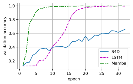
Mamba solves the task, and faster than the LSTM did. The mechanism we designed is that filler should collapse the learned \(\Delta_t\) toward zero, so the state carries the stored symbols forward untouched, while a marked symbol should open \(\Delta_t\) and write. Whether training found that mechanism is a measurable question, not one to assert: \(\Delta_t\) is an inference-time quantity, one forward pass away. The cell below pushes held-out sequences through the trained model and collects each block’s step sizes by token role.
mamba_copy.eval()
X = copy_data.X[copy_data.num_train:copy_data.num_train + 512].to(
    d2l.try_gpu())
with torch.no_grad():
    h, dts = mamba_copy.emb(X.T), []
    for blk in mamba_copy.encoder:
        u, _ = blk.W_in(blk.ln(h)).chunk(2, -1)
        u = blk.conv(u.permute(1, 2, 0))[..., :h.shape[0]]
        dt = F.softplus(blk.ssm.W_dt(F.silu(u.permute(2, 0, 1)))
                        + blk.ssm.b_dt)
        dts.append(d2l.numpy(dt.mean(-1)))  # Mean step size, (T, batch)
        h = blk(h)                          # On to the next block
roles = d2l.numpy(X.T)
masks = [roles == 0, roles >= 2, roles == 1]
fig, axes = d2l.plt.subplots(1, len(dts), figsize=(8, 3), sharey=True)
for i, (ax, dt) in enumerate(zip(axes, dts)):
    ax.boxplot([dt[m] for m in masks], showfliers=False)
    ax.set_xticks([1, 2, 3], ['filler', 'symbol', 'query'])
    ax.set_yscale('log')
    ax.set_title(f'block {i + 1}')
    ax.grid(linestyle='--', alpha=0.4)
axes[0].set_ylabel(r'learned $\Delta_t$ (channel mean)');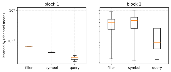
eval_copy = nnx.view(mamba_copy, deterministic=True,
                     use_running_average=True, raise_if_not_found=False)
X = jnp.asarray(copy_data.X[copy_data.num_train:copy_data.num_train + 512])
h, dts = eval_copy.emb(jax.nn.one_hot(X.T, eval_copy.vocab_size)), []
for blk in eval_copy.encoder.layers:
    u, _ = jnp.split(blk.W_in(blk.ln(h)), 2, axis=-1)
    u = jnp.swapaxes(blk.conv(jnp.swapaxes(u, 0, 1)), 0, 1)
    dt = jax.nn.softplus(blk.ssm.W_dt(jax.nn.silu(u)) + blk.ssm.b_dt)
    dts.append(d2l.numpy(dt.mean(-1)))      # Mean step size, (T, batch)
    h = blk(h)                              # On to the next block
roles = d2l.numpy(X.T)
masks = [roles == 0, roles >= 2, roles == 1]
fig, axes = d2l.plt.subplots(1, len(dts), figsize=(8, 3), sharey=True)
for i, (ax, dt) in enumerate(zip(axes, dts)):
    ax.boxplot([dt[m] for m in masks], showfliers=False)
    ax.set_xticks([1, 2, 3], ['filler', 'symbol', 'query'])
    ax.set_yscale('log')
    ax.set_title(f'block {i + 1}')
    ax.grid(linestyle='--', alpha=0.4)
axes[0].set_ylabel(r'learned $\Delta_t$ (channel mean)');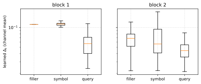
The trained step sizes separate by role: on filler tokens \(\Delta_t\) sits low, on the marked symbols it opens, and the query slots read out with their own regime. These measurements show that the trained model uses the step size as the proposed content-dependent gate. The content-dependent gating that Section 12.2.1 deleted to linearize the recurrence has been restored, not by putting the state back inside a nonlinearity, but by letting the input choose the coefficients of a linear map while preserving the affine structure required by the scan.
Selectivity follows from the state-space construction: begin with continuous dynamics, discretize them, and let the input set the step size. The next section (Section 12.4) starts over from the attention side, with the linear-attention recurrence of Section 10.5, and arrives at the same recurrence.
12.3.4 Summary
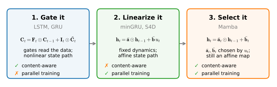
The chapter has developed three increasingly flexible state updates (Figure 12.3.3). Multiplicative gates let the data control writing, retention, and readout. Removing the nonlinearity from the state path turns the recurrence into an associative scan, while the state-space view supplies step-size gates, stable parameterizations, and memory constructions with formal guarantees. Making the step size and projections input-dependent restores content-dependent updates at the same asymptotic scan depth, although not at the same wall-clock cost. Our teaching implementation materializes the scan coefficients and therefore takes several times longer per epoch than the gated baselines in this experiment. The resulting Mamba block solved our selective-copy task, posted the best perplexity of the chapter in our PyTorch run (the minGRU edged it out in the JAX run), and, stepped one token at a time, generated text at constant cost per token from a state of a few kilobytes. What no update rule can change is that a fixed-size state at finite precision holds a fixed number of bits; what that limit costs, and how production systems buy it back with a few layers of attention, is where this chapter ends. First, though, comes a reckoning: the selective recurrence we built from ODEs and the attention we built in Chapter 10 are about to turn out to be the same computation (Section 12.4).
Experimental scope. The selective-copy runs are a diagnostic, built so that content-independent dynamics fail it. They show our S4D stack stalling and Mamba solving the same instance, with the measured \(\Delta_t\) separation as the mechanism; they do not show that no time-invariant model of any size could memorize a bounded version of the task. The capstone scoreboard is an illustration: one small corpus, one recipe per model, single seeded runs. It shows that the selective architecture can be trained to the best held-out perplexity at this scale, as it was in our PyTorch run, not a pound-for-pound ranking. The step-versus-scan agreement is an identity check on the trained network and holds to float tolerance in both frameworks.
12.3.5 Exercises
Additive scores. ● Write a selective-copying input of Section 12.3.1 as the token ids \(s_1, \ldots, s_T\) that precede the query slots. Call a model additive at a query slot if its vector of eight symbol logits there has the form
\[\mathbf{f}(s_1, \ldots, s_T) = \mathbf{c} + \sum_{t=1}^{T} \mathbf{g}_t(s_t),\]
where \(\mathbf{c} \in \mathbb{R}^8\) is a constant and each \(\mathbf{g}_t\) is an arbitrary map from token ids to \(\mathbb{R}^8\). The model answers correctly if the target symbol has the strictly largest logit.
- Remove the gated MLP from
S4DBlock, leaving the pre-norm, theS4Dlayer, and the residual connection, and place the result between a token embedding and a linear head. Show that this model is additive at every query slot. - Let
num_markedbe 1. Give an additive score that answers correctly wherever the single symbol appears. - Let
num_markedbe 3 and \(T = 4\), and let the query slot ask for the second of the three symbols. Prove that no additive score answers correctly on every placement. Restrict to inputs whose symbols are two fixed ids \(A\) and \(B\), and compare the logits of \(A\) and \(B\). - The two-block S4D stack of Section 12.3.1 is built from full
S4DBlocks. Show that a stack of two of the reduced blocks of the first part, with no gated MLP at all, is in general not additive, and name the operation responsible. Name the further operations of the fullS4DBlockthat have the same effect. Finally, explain why a single layer of Equation 12.3.2 is not additive.
- Remove the gated MLP from
Softplus step, sigmoid gate. Take one channel of the selective layer before discretization, that is, the continuous system Equation 12.2.5 with a single state (\(N = 1\)), \(a = -1\), and \(\mathbf{B}_t = 1\). Let the step size be \(\Delta_t = \textrm{softplus}(z_t)\) for a scalar pre-activation \(z_t\) computed from the input.
- Discretize with the exact zero-order hold Equation 12.2.8, and show that the update becomes \(x_t = (1 - g_t)\, x_{t-1} + g_t\, u_t\) with \(g_t = \sigma(z_t)\). This is Theorem 1 of Gu and Dao (2023) .
- Repeat the derivation with the first-order input rule \(\bar{\mathbf{B}}_t = \Delta_t \mathbf{B}_t\) that
SelectiveSSMuses. Show that both rules give an input weight of approximately \(e^{z_t}\) as \(z_t \to -\infty\), and compute the ratio of the two input weights at \(z_t \in \{-4, 0, 4\}\). - For a constant input \(u_t = u\), find the fixed point of the state under each rule, and state which rule keeps the state on the scale of the input as \(\Delta_t\) grows. Then let \(|u_t| \le U\) and \(z_t \le z_{\max}\) for all \(t\), start from \(x_0 = 0\), and bound \(|x_t|\) under each rule.
[code] Selective in \(\Delta\) only. ● The selective layer makes three quantities functions of the input: \(\boldsymbol{\Delta}_t\), \(\mathbf{B}_t\), and \(\mathbf{C}_t\). Measure which of them carries selective copying.
- Write two variants of
SelectiveSSM. In the first, only \(\boldsymbol{\Delta}_t\) depends on the input, while \(\mathbf{B} = \mathbf{1}\) is fixed and \(\mathbf{C}\) is a learned \((H, N)\) parameter as inS4D. In the second, \(\Delta\) is a learned per-channel constant as inS4D, while \(\mathbf{B}_t\) and \(\mathbf{C}_t\) remain functions of the input. Before training, predict from the gate interpretation of Section 12.2.3.1 and from problem 2 which variant solves the task within the budget oftrain_copy. - Build the architecture of
mamba_copy, replace thessmattribute of eachMambaBlockby a variant, and train each withtrain_copy. Plot the two curves together with those of the S4D, the LSTM, and the full Mamba. Which ingredient carries the task? - Gu and Dao (2023) run the corresponding ablation in a language model and report perplexities of 10.93 with none of the three input-dependent, 10.15 with \(\mathbf{B}\) alone, 9.98 with \(\mathbf{C}\) alone, 9.81 with \(\Delta\) alone, and 8.71 with all three. Which of these settings matches your first variant, and why does none match your second? Is the ingredient that carries selective copying the one that their ablation ranks first among single ingredients?
- Write two variants of
Linear or time-invariant. An LTI system is both linear and time invariant, and Section 12.3.2.2 states that selectivity removes the convolution view. Consider one
SelectiveSSMlayer as a map from an input sequence \(\mathbf{u}_1, \ldots, \mathbf{u}_T\) to an output sequence, started from the zero state.- Show that prepending \(k\) zero vectors to the input prepends \(k\) zero vectors to the output and leaves the remaining outputs unchanged.
- Show that the layer is not linear in its input by computing the output at \(t = 1\) for the inputs \(\mathbf{u}_1\) and \(2\mathbf{u}_1\).
- Prove that a causal map that is linear and commutes with the shift of the first part is a convolution \(\mathbf{y}_t = \sum_{k \ge 0} \bar{\mathbf{K}}_k \mathbf{u}_{t-k}\).
- Fix one input sequence and treat the \(\boldsymbol{\Delta}_t\), \(\mathbf{B}_t\), and \(\mathbf{C}_t\) it produces as constants. Write the output of channel \(h\) as \(y_{t,h} = \sum_{s \le t} M_{t,s}\, u_{s,h} + d_h u_{t,h}\), and give \(M_{t,s}\). Show that \(M_{t,s}\) is in general not a function of \(t - s\) alone, and explain why the FFT of Section 12.2.3.2 cannot evaluate this sum even after the input, and hence \(M\), is known.
Materialized scan memory. Table 12.3.1 records that our
SelectiveSSMmaterializes coefficient tensors of shape \((T, \textrm{batch}, H, N)\). Take oneMambaBlockof the language model of Section 12.3.3.1: \(T = 32\), a batch of 1024 windows, model width 128 and hence \(H = 256\) after expansion, \(N = 4\), and float32 entries.- Compute the size of one such tensor. Suppose that the scan follows the doubling schedule of Figure 12.2.1 and that the backward pass keeps the decay and input tensors entering each of the \(\lceil \log_2 T \rceil\) rounds, plus the scan output. Compute the memory that the scan keeps per block.
- A fused kernel keeps only \(\mathbf{u}_t\) and \(\boldsymbol{\Delta}_t\), each of shape \((T, \textrm{batch}, H)\), and \(\mathbf{B}_t\) and \(\mathbf{C}_t\), each of shape \((T, \textrm{batch}, N)\), and recomputes everything else during the backward pass. Compute its storage and the ratio to the previous part. Express the ratio in terms of \(T\), \(H\), and \(N\), and evaluate it at \(N = 16\), \(T = 2048\), and \(H = 4096\).
S4Dpasses its decays to the same scan with a batch axis of size one, because they do not depend on the input. Under the assumption of the first part, compute the memory that its scan keeps for the same shapes. Which part of the selective layer’s storage is the price of selectivity?
Block parameter budget. Let a
MambaBlockhave model width \(d\), expansion \(E\), \(N\) states, convolution width \(w\), and a rank-\(R\) head for \(\boldsymbol{\Delta}_t\), so that itsSelectiveSSMhas width \(Ed\).- Count the parameters of one block, biases and normalization included, as a function of \(d\), \(E\), \(N\), \(R\), and \(w\). Show that at fixed \(R\) the leading term in \(d\) is the \(3Ed^2\) of Gu and Dao (2023), and identify the matrices that contribute it.
SelectiveSSMsets \(R = Ed/16\); find the quadratic term that the \(\boldsymbol{\Delta}_t\) head then adds. - Evaluate the count for the blocks of
Mamba(num_inputs=128)in Section 12.3.3.1, where \(E = 2\), \(N = 4\), \(R = 16\), and \(w = 4\). Give the fractions of the block held by the two projections and by the selective SSM. Add the embedding and the output layer for the 1024-token vocabulary, compare the total with the parameter count thatbenchmarkrecords in Section 12.3.3.1, and give the share of the model’s parameters that lies outside the Mamba blocks. - A transformer block of width \(d\) holds about \(12d^2\) parameters (Section 11.1). How many Mamba blocks with \(E = 2\) match one transformer block, and what does this imply when comparing the depths of the two architectures at equal parameter count?
- Count the parameters of one block, biases and normalization included, as a function of \(d\), \(E\), \(N\), \(R\), and \(w\). Show that at fixed \(R\) the leading term in \(d\) is the \(3Ed^2\) of Gu and Dao (2023), and identify the matrices that contribute it.
[code] Prefill and decode. ●
stepped_fnof Section 12.3.3.2 plays the prompt into the state one token at a time, while the parallel forward pass ofMambacomputes the same states with the scan and returnsNoneas its state.- Modify the forward passes of
SelectiveSSM,MambaBlock, andMambaso that they also return, for every block, the pair of convolution buffer and SSM state thatMambaBlock.stepholds after the last token, in the layout thatstepexpects. Prefill a prompt with one forward pass, decode the continuation withstep, and verify on the trainedmamba_lmthat the logits agree with pure stepping to float tolerance. - Time the prefill of prompts of \(P \in \{32, 256, 2048\}\) tokens, once with the scan and once by stepping, and time the decoding of each further token. How do the two prefill times scale with \(P\), and does the time per decoded token depend on \(P\)? Relate the result to the split between prefill and decode of Section 11.3.
- Modify the forward passes of
[code] Interventions on \(\Delta\). ● The step-size measurement of Section 12.3.3.3 shows that \(\Delta_t\) separates by token role in the trained
mamba_copy. A correlation does not show that the model’s answers depend on this separation, but an intervention can.- Extend the measurement code into a forward pass of the trained model in which each block computes its SSM from a step size that you supply. Check that supplying each block’s own \(\Delta_t\) reproduces the model’s validation accuracy.
- In every block, replace \(\Delta_t\) at filler positions by the channel’s median \(\Delta\) over symbol positions, and measure the accuracy. Then replace \(\Delta_t\) at symbol positions by the channel’s median over filler positions. Predict both accuracies before running, and explain each outcome by what the state does at the affected tokens.
- Apply each intervention to one block at a time. Which block’s step size does the answer depend on, and does that agree with the box plots of Section 12.3.3.3?
[code] Longer filler runs. The models
s4d,lstm, andmamba_copywere trained on sequences of 256 tokens before the query slots. None of them uses position embeddings, so each runs on sequences of any length.- Build validation sets with
SelectiveCopyatnum_steps\(\in \{1024, 4096\}\), use the validation split ofcopy_datafor 256, and report the accuracy of the three trained models at each length without retraining. Evaluate in batches of 64 sequences, because the scan materializes \((T, \textrm{batch}, H, N)\) tensors. - Over a run of filler tokens, the decay alone multiplies state coordinate \(n\) of a channel by \(\exp\bigl(-|a_n| \sum_t \Delta_t\bigr)\), the sum running over the run. From the trained
log_aand each channel’s median \(\Delta\) on filler, measured as in Section 12.3.3.3, compute this factor for each channel’s slowest mode over runs of 256 and 4096 filler tokens. Use the distribution of the factor over channels to explain the accuracies of the first part. - Gu and Dao (2023) report that a Mamba trained on an induction-head task at length 256 extrapolates to sequences of a million tokens. Which property of the learned \(\Delta_t\) would such extrapolation require, and does your measurement show it?
- Build validation sets with
[extended] Block ablations. ● Besides the selective SSM, the block of Figure 12.3.2 has three ingredients: the short causal convolution, the SiLU on the main branch, and the gate branch.
- Build three variants of
MambaBlock: one without the gate, which passes the SSM output straight toW_out; one without the convolution, withconv_width=1; and one with the identity in place of the SiLU in front of the SSM. - Train each variant on selective copying with
train_copy, and as a two-block stack in the language model of Section 12.3.3.1 withbenchmark, keeping each task’s recipe. - Which change hurts most on each task? For the variant without the convolution, explain from Equation 12.3.1 what information \(\boldsymbol{\Delta}_t\), \(\mathbf{B}_t\), and \(\mathbf{C}_t\) lose in the first block, and why later blocks lose less.
- Build three variants of
- [code] Causality test. A causal sequence model must leave its output at position \(s\) unchanged when the input at a later position \(t > s\) changes.
- Write a test that perturbs
X[t]of a random input toMamba(num_inputs=32)and reports which output positions change. MambaBlock.forwardpads both ends of the sequence byconv_width - 1and keeps the firstX.shape[0]outputs of the convolution. Keep the lastX.shape[0]outputs instead. Before running your test, determine how many future tokens each output now sees, and then confirm it with the test.- Build the language model of Section 12.3.3.1 from the modified
Mamba, run the step-versus-scan check of Section 12.3.3.2 on it without training, and explain its result.
- Write a test that perturbs
- [code] Causality test. A causal sequence model must leave its output at position \(s\) unchanged when the input at a later position \(t > s\) changes.
- Write a test that perturbs
X[t]of a random input toMamba(num_inputs=32)and reports which output positions change. MambaBlockbuilds its convolution withpadding='CAUSAL'. Build it withpadding='SAME'instead. Before running your test, determine how many future tokens each output now sees, and then confirm it with the test.- Build the language model of Section 12.3.3.1 from the modified
Mamba, run the step-versus-scan check of Section 12.3.3.2 on it without training, and explain its result.
- Write a test that perturbs