%matplotlib inline
from d2l import torch as d2l
import torch
import math25.2 Multivariable Calculus
A deep network’s loss depends on many parameters. Section 25.1 described the response to a change in one variable; here we extend the local linear approximation to several variables. The gradient represents the first-order derivative and determines directions of steepest change. Applying the multivariable chain rule efficiently gives backpropagation. We conclude with the Hessian, whose second-order information distinguishes minima, maxima, and saddle points.
25.2.1 From Partial Derivatives to the Gradient
25.2.1.1 Partial Derivatives
If we change a single weight \(w_1\) and freeze the rest, we are back to a function of one variable, and Section 25.1 applies directly:
\[L(w_1+\epsilon_1, w_2, \ldots, w_N) \approx L(w_1, w_2, \ldots, w_N) + \epsilon_1 \frac{\partial}{\partial w_1} L(w_1, w_2, \ldots, w_N). \tag{25.2.1}\]
The derivative in one variable while holding the others fixed is the partial derivative, written \(\frac{\partial}{\partial w_1}\). The new idea is what happens when we perturb several coordinates at once.
25.2.1.2 The Gradient
Assume first that \(L\) is differentiable at \(\mathbf w\). By definition, its change under a joint perturbation \(\boldsymbol\epsilon\) equals a linear function plus an error \(o(\|\boldsymbol\epsilon\|)\). In Euclidean coordinates that linear function is a dot product with some vector \(\mathbf g\). Setting \(\boldsymbol\epsilon=h\mathbf e_i\) identifies \(g_i\) with \(\partial L/\partial w_i\). Thus differentiability gives
\[ L(w_1+\epsilon_1, \ldots, w_N+\epsilon_N) \approx L(w_1, \ldots, w_N) + \sum_{i=1}^N \epsilon_i \frac{\partial L}{\partial w_i}. \]
That sum on the right is a dot product. Collecting the perturbations and the partials into vectors,
\[ \boldsymbol{\epsilon} = [\epsilon_1, \ldots, \epsilon_N]^\top \quad\textrm{and}\quad \nabla_{\mathbf{w}} L = \left[\frac{\partial L}{\partial w_1}, \ldots, \frac{\partial L}{\partial w_N}\right]^\top, \]
we obtain the multivariable analogue of the linear approximation,
\[L(\mathbf{w} + \boldsymbol{\epsilon}) \approx L(\mathbf{w}) + \boldsymbol{\epsilon}\cdot \nabla_{\mathbf{w}} L(\mathbf{w}). \tag{25.2.2}\]
The vector \(\nabla_{\mathbf{w}} L\) is the gradient of \(L\). Equation Equation 25.2.2 has exactly the shape of the one-dimensional \(f(x+\epsilon) \approx f(x) + \epsilon f'(x)\), with the scalar derivative replaced by the gradient and ordinary multiplication replaced by a dot product. The gradient is the derivative in many dimensions: it is the unique vector whose dot product with a perturbation gives the first-order change in \(L\). We treat \(\nabla_{\mathbf{w}} L\) as a column vector throughout; the layout conventions that make this choice precise are settled in Section 25.3.
This order of reasoning matters. Existence of all partial derivatives does not itself imply the joint linear approximation. A convenient sufficient condition is that the partials exist and are continuous near \(\mathbf w\). For a counterexample, \(f(x, y) = 2xy/(x^2+y^2)\) with \(f(0,0) = 0\) has both partials equal to zero at the origin, yet equals \(1\) everywhere on the diagonal \(x = y \neq 0\), so no linear approximation can hold there.
25.2.1.3 Directional Derivatives
Reading Equation 25.2.2 for a perturbation \(\boldsymbol{\epsilon} = h\,\mathbf{u}\) of size \(h\) along a unit direction \(\mathbf{u}\) shows how the gradient determines the derivative in any direction:
\[ \frac{L(\mathbf{w} + h\,\mathbf{u}) - L(\mathbf{w})}{h} \;\xrightarrow{\;h\to 0\;}\; \mathbf{u}\cdot\nabla_{\mathbf{w}} L(\mathbf{w}). \]
The rate of change of \(L\) as we move along \(\mathbf{u}\) is the projection of the gradient onto \(\mathbf{u}\), and that rate is the directional derivative. The single vector \(\nabla_{\mathbf{w}} L\) thus encodes the slope in every direction simultaneously. The next section turns this one identity into the geometry of gradient descent.
First, let us check that Equation 25.2.2 really does approximate \(L\).
%matplotlib inline
from d2l import tensorflow as d2l
import tensorflow as tf
import math%matplotlib inline
from d2l import jax as d2l
import jax
from jax import numpy as jnp
import math%matplotlib inline
from d2l import mxnet as d2l
from mxnet import autograd, np, npx
import math
npx.set_np()Take
\[ f(x, y) = \log(e^x + e^y), \qquad \nabla f (x, y) = \left[\frac{e^x}{e^x+e^y}, \frac{e^y}{e^x+e^y}\right]^\top. \]
At the point \((0, \log 2)\) we have \(f = \log 3\) and \(\nabla f = [\tfrac13, \tfrac23]^\top\), so Equation 25.2.2 predicts \(f(\epsilon_1, \log 2 + \epsilon_2) \approx \log 3 + \tfrac13\epsilon_1 + \tfrac23\epsilon_2\). We compare this against the true value for a small step. The check is plain scalar arithmetic.
def f(x, y):
    return math.log(math.exp(x) + math.exp(y))

def grad_f(x, y):
    s = math.exp(x) + math.exp(y)
    return [math.exp(x) / s, math.exp(y) / s]

epsilon = [0.01, -0.03]
x0, y0 = 0, math.log(2)
approx = f(x0, y0) + sum(e * g for e, g in zip(epsilon, grad_f(x0, y0)))
true_value = f(x0 + epsilon[0], y0 + epsilon[1])
print(f'approximation: {approx:.6f}, true value: {true_value:.6f}')
approximation: 1.081946, true value: 1.082124The two agree to about three decimal places, with a gap of \(1.8\times10^{-4}\). The gap is not noise, and its size is itself a lesson: a first-order model discards terms of order \(\|\boldsymbol{\epsilon}\|^2\), and here \(\|\boldsymbol{\epsilon}\|^2 = 10^{-3}\): shrink the step tenfold and the gap shrinks a hundredfold. The discarded term has a name and a formula (the Hessian quadratic \(\tfrac12\boldsymbol{\epsilon}^\top\mathbf{H}f\,\boldsymbol{\epsilon}\)), which we develop at the end of this section.
The same example illustrates a standard verification procedure: compare a hand-derived gradient against automatic differentiation. Here autograd should reproduce \(\nabla f(0, \log 2) = [\tfrac13, \tfrac23]^\top\).
# Check the hand-derived gradient at (0, log 2): [1/3, 2/3]
xy = torch.tensor([0.0, math.log(2)], requires_grad=True)
torch.logsumexp(xy, 0).backward()
print(f'autograd gradient: {xy.grad}')
autograd gradient: tensor([0.3333, 0.6667])# Check the hand-derived gradient at (0, log 2): [1/3, 2/3]
xy = tf.Variable([0.0, math.log(2.0)])
with tf.GradientTape() as t:
out = tf.reduce_logsumexp(xy)
print(f'autograd gradient: {t.gradient(out, xy).numpy()}')autograd gradient: [0.33333334 0.6666667 ]# Check the hand-derived gradient at (0, log 2): [1/3, 2/3]
grad = jax.grad(jax.scipy.special.logsumexp)(jnp.array([0.0, math.log(2.0)]))
print(f'autograd gradient: {grad}')autograd gradient: [0.33333334 0.6666667 ]# Check the hand-derived gradient at (0, log 2): [1/3, 2/3]
xy = np.array([0.0, math.log(2)])
xy.attach_grad()
with autograd.record():
out = np.log(np.exp(xy).sum())
out.backward()
print(f'autograd gradient: {xy.grad}')autograd gradient: [0.33333334 0.6666667 ][14:00:04] /home/smola/mxnet/src/base.cc:48: GPU context requested, but no GPUs found.Up to display precision, the printout is our hand-computed \([\tfrac13, \tfrac23]^\top\).
25.2.2 The Geometry of Gradients
25.2.2.1 Steepest Descent
Equation Equation 25.2.2 tells us how \(L\) changes in any direction, so we can ask which direction makes it decrease fastest. This is the geometric content of gradient descent, first introduced in Section 2.1:
- Start from some initial parameters \(\mathbf{w}\).
- Find the unit direction \(\mathbf{v}\) along which \(L\) decreases most rapidly.
- Take a small step that way: \(\mathbf{w} \leftarrow \mathbf{w} + \eta\mathbf{v}\).
- Repeat.
To solve step 2, write the gradient’s effect on a unit direction \(\mathbf{v}\) using the geometric form of the dot product from Section 24.1,
\[ L(\mathbf{w} + \mathbf{v}) - L(\mathbf{w}) \approx \mathbf{v}\cdot \nabla_{\mathbf{w}} L(\mathbf{w}) = \|\nabla_{\mathbf{w}} L(\mathbf{w})\|\cos(\theta), \]
where \(\theta\) is the angle between \(\mathbf{v}\) and the gradient. The direction enters only through \(\cos\theta\).
Proposition (steepest ascent and descent). At any point where \(\nabla L \neq \mathbf{0}\), among all unit vectors \(\mathbf{v}\) the directional derivative \(\mathbf{v}\cdot\nabla L\) is largest when \(\mathbf{v}\) points along \(+\nabla L\) and smallest when it points along \(-\nabla L\). Thus \(+\nabla L\) is the direction of steepest ascent and \(-\nabla L\) the direction of steepest descent.
Here “unit” and “steepest” refer to the Euclidean norm and its inner product. With a different norm, the unit ball changes and the minimizing direction is determined by the corresponding dual norm; it need not be the negative Euclidean gradient.
Proof. By Cauchy–Schwarz (Equation 24.1.4) applied to the unit vector \(\mathbf{v}\),
\[ -\|\nabla L\| \;\le\; \mathbf{v}\cdot\nabla L \;\le\; \|\nabla L\|, \]
and the Cauchy–Schwarz equality criterion (equality holds exactly for collinear vectors) says each bound is attained exactly when \(\mathbf{v}\) is collinear with \(\nabla L\). The upper bound \(+\|\nabla L\|\) is reached by \(\mathbf{v} = \nabla L/\|\nabla L\|\) and the lower bound \(-\|\nabla L\|\) by \(\mathbf{v} = -\nabla L/\|\nabla L\|\). \(\blacksquare\)
In the \(\cos\theta\) picture this is simply \(\theta = 0\) versus \(\theta = \pi\). Steepest descent therefore steps along \(-\nabla_{\mathbf{w}} L\), and the informal recipe becomes the gradient-descent update
\[ \mathbf{w} \leftarrow \mathbf{w} - \eta\,\nabla_{\mathbf{w}} L(\mathbf{w}). \]
First-order optimizers use gradient information, but they need not step along the current negative gradient. Momentum combines gradients across time, while RMSProp and Adam rescale coordinates; Chapter 9 develops the resulting directions.
25.2.2.2 Gradients and Level Sets
The same expression \(L(\mathbf{w} + \mathbf{v}) - L(\mathbf{w}) \approx \|\nabla L\|\cos\theta\) also reveals what the gradient is geometrically, not just which way to step. Consider moving along a level set, the set of points where \(L\) keeps a fixed value \(c\). To first order, \(L\) does not change along such a direction, so the directional derivative vanishes.
Proposition (gradients are normal to level sets). At any point, \(\nabla L\) is orthogonal to every direction tangent to the level set \(\{\mathbf{x} : L(\mathbf{x}) = c\}\) through that point.
Proof. A direction \(\mathbf{v}\) is tangent to the level set at \(\mathbf{x}\) if \(\mathbf{v} = \boldsymbol{\gamma}'(0)\) for some differentiable curve \(\boldsymbol{\gamma}(t)\) lying in the level set with \(\boldsymbol{\gamma}(0) = \mathbf{x}\). Along such a curve \(L(\boldsymbol{\gamma}(t)) = c\) for all \(t\), so the derivative of \(t \mapsto L(\boldsymbol{\gamma}(t))\) at \(t = 0\) vanishes. To first order \(\boldsymbol{\gamma}(t) = \mathbf{x} + t\mathbf{v} + o(t)\), so by Equation 25.2.2 that derivative is \(\mathbf{v}\cdot\nabla L(\mathbf{x})\). Hence \(\mathbf{v}\cdot\nabla L = 0\); by the definition of orthogonality from Section 24.1, \(\mathbf{v}\perp\nabla L\). \(\blacksquare\)
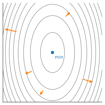
On a contour map, the gradient crosses each contour at a right angle and points toward increasing values. Its norm is largest where \(L\) changes fastest, as shown in Figure 25.2.1. Gradient descent moves in the opposite direction, perpendicular to the contours.
25.2.2.3 Tangent Planes and Linearization
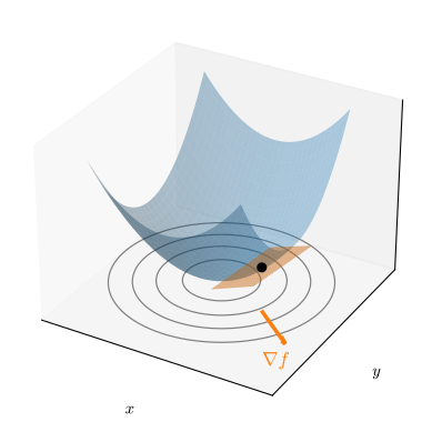
A level-set diagram represents the domain in the base plane, with the gradient normal to each contour. The graph \(z = f(\mathbf{x})\) gives a second representation one dimension higher. Reading Equation 25.2.2 as an equation for the height \(z\) rather than as an approximation gives the linearization of \(f\) at \(\mathbf{x}_0\),
\[ z = f(\mathbf{x}_0) + \nabla f(\mathbf{x}_0)\cdot(\mathbf{x}-\mathbf{x}_0), \tag{25.2.3}\]
a linear function of \(\mathbf{x}\) whose graph is a plane (a hyperplane in higher dimensions). It passes through the point \((\mathbf{x}_0, f(\mathbf{x}_0))\) and matches every first-order slope of \(f\) there, so it is the tangent plane to the surface: the two-dimensional analogue of the tangent line, and the surface’s best linear approximation near \(\mathbf{x}_0\).
Rewrite Equation 25.2.3 as \(\nabla f(\mathbf{x}_0)\cdot(\mathbf{x}-\mathbf{x}_0) - (z - f(\mathbf{x}_0)) = 0\): this says the augmented vector \([\nabla f(\mathbf{x}_0),\, -1]^\top\) is normal, in graph space, to the tangent plane; the gradient is normal to the surface once we account for the height direction. Drop the height coordinate, projecting that normal onto the base plane, and we recover \(\nabla f\) crossing the level curves at right angles. Figure 25.2.2 shows the tangent plane together with this projected gradient.
25.2.2.4 Critical Points and the First-Order Test
Throughout this book we minimize losses numerically, because the functions that arise in deep learning are far too complex to minimize in closed form. But the geometry above gives a cheap, exact necessary condition that every minimum must satisfy.
A necessary condition can reject a proposed minimizer of \(L\) at \(\mathbf{x}_0\). Applying Equation 25.2.2 at \(\mathbf{x}_0\), if \(\nabla L(\mathbf{x}_0) \neq \mathbf{0}\), then stepping along \(-\nabla L(\mathbf{x}_0)\) strictly decreases \(L\), so \(\mathbf{x}_0\) cannot be a minimum. Contrapositively, a minimum forces \(\nabla L(\mathbf{x}_0) = \mathbf{0}\). Points where the gradient vanishes are called critical points.
This is occasionally enough to optimize by hand. For example,
\[ f(x) = 3x^4 - 4x^3 - 12x^2, \qquad f'(x) = 12x(x-2)(x+1), \]
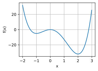
has critical points \(x = -1, 0, 2\) with values \(-5, 0, -32\), so the minimum is at \(x = 2\), as the plot confirms.
import numpy as onp
x = onp.arange(-2, 3, 0.01)
f = (3 * x**4) - (4 * x**3) - (12 * x**2)

d2l.plot(x, f, 'x', 'f(x)')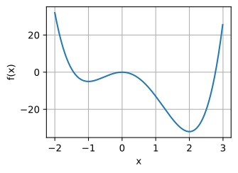
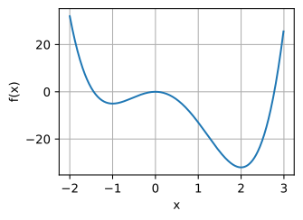
But not every critical point is an extremum: \(x = 0\) above is a local maximum, and in higher dimensions a critical point can be a saddle. Telling these apart needs second-order information, the Hessian we develop below.
25.2.2.5 Optimizing on a Constraint
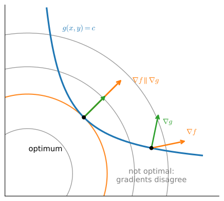
The first-order test answers “where can an unconstrained minimum be?” One more turn of the same geometry answers the constrained question that pervades machine learning: minimize a loss subject to keeping some quantity fixed, say \(g(\mathbf{x}) = c\). Now we are no longer free to step in any direction: the admissible moves are exactly those tangent to the constraint surface \(\{g = c\}\). At a constrained optimum \(\mathbf{x}^\star\), no admissible direction can lower \(f\) to first order: otherwise we would slide along the constraint and improve. By Equation 25.2.2 that means \(\nabla f(\mathbf{x}^\star)\) has zero component along every direction tangent to \(\{g = c\}\); it is orthogonal to that surface. But we proved above that \(\nabla g\) is also orthogonal to \(\{g = c\}\). One hypothesis makes the geometry rigorous: provided \(\nabla g(\mathbf{x}^\star) \neq \mathbf{0}\), the standard constraint qualification, the implicit function theorem (stated in Section 25.3.4.6; see (Rudin 1976)) guarantees that \(\{g = c\}\) really is a smooth surface of codimension one near \(\mathbf{x}^\star\) (one equation removes one degree of freedom, leaving an \((n{-}1)\)-dimensional surface) with a single normal direction; it also supplies the fact, used tacitly above, that every tangent direction is realized by a curve lying in \(\{g = c\}\), so “sliding along the constraint” is a legitimate move. Two vectors normal to the same surface must be parallel, so at the constrained optimum
\[ \nabla f(\mathbf{x}^\star) = \lambda\,\nabla g(\mathbf{x}^\star) \tag{25.2.4}\]
for some scalar \(\lambda\), the Lagrange multiplier. This single picture is the first-order condition for constrained optimization and a basis for the KKT conditions and duality. At the solution, a contour of \(f\) is tangent to the constraint surface and their gradients align (Figure 25.2.3). Section 26.4 develops this condition further.
25.2.3 The Multivariate Chain Rule
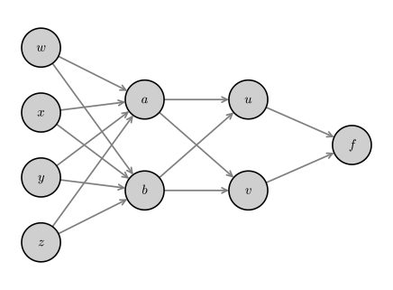
Neural networks are deep compositions of simple functions, so computing gradients means differentiating compositions. Consider four inputs \(w, x, y, z\) flowing through intermediate quantities to a scalar output:
\[\begin{aligned}f(u, v) & = (u+v)^{2} \\u(a, b) & = (a+b)^{2}, \qquad v(a, b) = (a-b)^{2}, \\a(w, x, y, z) & = (w+x+y+z)^{2}, \qquad b(w, x, y, z) = (w+x-y-z)^2.\end{aligned} \tag{25.2.5}\]
The dependencies form a graph (Figure 25.2.4): each node is a value, each edge a direct functional dependence.
Direct substitution produces long expressions with repeated subexpressions; computing another partial derivative repeats much of the same work. The chain rule organizes these shared computations.
25.2.3.1 The Rule as a Sum Over Paths
Take the simplest composite step, \(f(u(a,b), v(a,b))\), and perturb \(a\) by a small \(\epsilon\). Each intermediate moves by its partial, \(u \to u + \epsilon\frac{\partial u}{\partial a}\) and \(v \to v + \epsilon\frac{\partial v}{\partial a}\), and feeding those into the first-order expansion of \(f\) gives
\[ f\!\left(u + \epsilon\tfrac{\partial u}{\partial a},\, v + \epsilon\tfrac{\partial v}{\partial a}\right) \approx f(u, v) + \epsilon\left[\frac{\partial f}{\partial u}\frac{\partial u}{\partial a} + \frac{\partial f}{\partial v}\frac{\partial v}{\partial a}\right]. \]
Reading off the coefficient of \(\epsilon\) gives the multivariate chain rule,
\[ \frac{\partial f}{\partial a} = \frac{\partial f}{\partial u}\frac{\partial u}{\partial a} + \frac{\partial f}{\partial v}\frac{\partial v}{\partial a}. \]
In words, there are two pathways by which \(a\) influences \(f\): \(a \to u \to f\) and \(a \to v \to f\). Each path contributes the product of the derivatives along its edges, and the total derivative is the sum over paths.
In general, to differentiate the output with respect to an input we sum, over every directed path from that input to the output, the product of the edge derivatives along the path.
To see the rule at work on a graph that is not a tree, consider a different composition (its own dependency graph, unrelated to Equation 25.2.5) in which one intermediate feeds the output both directly and through a later node:
\[\begin{aligned}u(x, y) & = x + y, \qquad v(x, y) = x - y, \\a(u) & = u^2, \qquad b(v) = v^2, \\f(a, u, b) & = a + u + b.\end{aligned} \tag{25.2.6}\]
These relations are exactly the edges drawn in Figure 25.2.5: \(u\) and \(v\) each depend on the input \(y\); \(a\) depends on \(u\) and \(b\) on \(v\); and the output \(f\) depends on \(a\), on \(b\), and also directly on \(u\): the skip-like edge that gives the middle path below. Tracing every directed route from \(y\) to \(f\) (namely \(y\to u\to a\to f\), the direct \(y\to u\to f\), and \(y\to v\to b\to f\)), the rule gives
\[ \frac{\partial f}{\partial y} = \frac{\partial f}{\partial a} \frac{\partial a}{\partial u} \frac{\partial u}{\partial y} + \frac{\partial f}{\partial u} \frac{\partial u}{\partial y} + \frac{\partial f}{\partial b} \frac{\partial b}{\partial v} \frac{\partial v}{\partial y}. \]
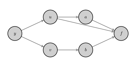
Here every edge derivative is elementary (\(\partial f/\partial a = \partial f/\partial u = \partial f/\partial b = 1\), \(\partial a/\partial u = 2u\), \(\partial u/\partial y = 1\), and so on), so the sum-over-paths value is checkable by hand: it collapses to \(2u + 1 - 2v = 2(x+y) + 1 - 2(x-y) = 1 + 4y\). This “sum over paths” view is exactly how gradients flow through a network, and it explains why architectural choices that open or close paths, such as the gates of an LSTM (Section 12.1) or the skip connections of a residual block (Section 7.4), shape learning by controlling that gradient flow.
25.2.3.2 The Backpropagation Algorithm
Return to Equation 25.2.5 and ask for \(\frac{\partial f}{\partial w}\). Expanding the chain rule directly pushes \(w\) forward through the graph,
\[ \frac{\partial f}{\partial w} = \frac{\partial f}{\partial u}\frac{\partial u}{\partial w} + \frac{\partial f}{\partial v}\frac{\partial v}{\partial w}, \qquad \frac{\partial u}{\partial w} = \frac{\partial u}{\partial a}\frac{\partial a}{\partial w}+\frac{\partial u}{\partial b}\frac{\partial b}{\partial w}, \quad \ldots \]
and the single-step partials are all elementary,
\[ \begin{aligned} \frac{\partial f}{\partial u} = 2(u+v), & \quad\frac{\partial f}{\partial v} = 2(u+v), \\ \frac{\partial u}{\partial a} = 2(a+b), & \quad\frac{\partial u}{\partial b} = 2(a+b), \\ \frac{\partial v}{\partial a} = 2(a-b), & \quad\frac{\partial v}{\partial b} = -2(a-b), \\ \frac{\partial a}{\partial w} = 2(w+x+y+z), & \quad\frac{\partial b}{\partial w} = 2(w+x-y-z). \end{aligned} \]
In code this is a tidy forward sweep through the graph.
# Compute the value of the function from inputs to outputs
w, x, y, z = 1, 1, -2, 1
a, b = (w + x + y + z)**2, (w + x - y - z)**2
u, v = (a + b)**2, (a - b)**2
f = (u + v)**2
print(f'f at {w}, {x}, {y}, {z} is {f}')

# Compute the single step partials
df_du, df_dv = 2*(u + v), 2*(u + v)
du_da, du_db, dv_da, dv_db = 2*(a + b), 2*(a + b), 2*(a - b), -2*(a - b)
da_dw, db_dw = 2*(w + x + y + z), 2*(w + x - y - z)

# Compute the final result from inputs to outputs
du_dw, dv_dw = du_da*da_dw + du_db*db_dw, dv_da*da_dw + dv_db*db_dw
df_dw = df_du*du_dw + df_dv*dv_dw
print(f'df/dw at {w}, {x}, {y}, {z} is {df_dw}')
f at 1, 1, -2, 1 is 26896
df/dw at 1, 1, -2, 1 is 73472This computes \(\frac{\partial f}{\partial w}\) but does not reuse the calculation for \(\frac{\partial f}{\partial x}\). Deep learning instead requires the derivative of one loss with respect to every parameter. We therefore keep \(\partial f\) in each numerator and traverse the graph backward from the output:
\[ \begin{aligned} \frac{\partial f}{\partial a} & = \frac{\partial f}{\partial u}\frac{\partial u}{\partial a}+\frac{\partial f}{\partial v}\frac{\partial v}{\partial a}, \qquad \frac{\partial f}{\partial b} = \frac{\partial f}{\partial u}\frac{\partial u}{\partial b}+\frac{\partial f}{\partial v}\frac{\partial v}{\partial b}, \\ \frac{\partial f}{\partial w} & = \frac{\partial f}{\partial a}\frac{\partial a}{\partial w} + \frac{\partial f}{\partial b}\frac{\partial b}{\partial w}, \qquad (\textrm{and likewise for } x, y, z). \end{aligned} \]
Computing \(\frac{\partial f}{\partial u}, \frac{\partial f}{\partial v}\) once, then \(\frac{\partial f}{\partial a}, \frac{\partial f}{\partial b}\), then all four input derivatives, reuses every intermediate. One backward sweep yields the gradient with respect to all inputs at once.
# Compute the value of the function from inputs to outputs
w, x, y, z = 1, 1, -2, 1
a, b = (w + x + y + z)**2, (w + x - y - z)**2
u, v = (a + b)**2, (a - b)**2
f = (u + v)**2
print(f'f at {w}, {x}, {y}, {z} is {f}')

# Compute the derivative using the decomposition above
# First compute the single step partials
df_du, df_dv = 2*(u + v), 2*(u + v)
du_da, du_db, dv_da, dv_db = 2*(a + b), 2*(a + b), 2*(a - b), -2*(a - b)
da_dw, db_dw = 2*(w + x + y + z), 2*(w + x - y - z)
da_dx, db_dx = 2*(w + x + y + z), 2*(w + x - y - z)
da_dy, db_dy = 2*(w + x + y + z), -2*(w + x - y - z)
da_dz, db_dz = 2*(w + x + y + z), -2*(w + x - y - z)

# Now compute how f changes when we change any value from output to input
df_da, df_db = df_du*du_da + df_dv*dv_da, df_du*du_db + df_dv*dv_db
df_dw, df_dx = df_da*da_dw + df_db*db_dw, df_da*da_dx + df_db*db_dx
df_dy, df_dz = df_da*da_dy + df_db*db_dy, df_da*da_dz + df_db*db_dz

print(f'df/dw at {w}, {x}, {y}, {z} is {df_dw}')
print(f'df/dx at {w}, {x}, {y}, {z} is {df_dx}')
print(f'df/dy at {w}, {x}, {y}, {z} is {df_dy}')
print(f'df/dz at {w}, {x}, {y}, {z} is {df_dz}')
f at 1, 1, -2, 1 is 26896
df/dw at 1, 1, -2, 1 is 73472
df/dx at 1, 1, -2, 1 is 73472
df/dy at 1, 1, -2, 1 is -68224
df/dz at 1, 1, -2, 1 is -68224Two sanity checks are visible in the printout. The derivatives with respect to \(w\) and \(x\) agree, as do those with respect to \(y\) and \(z\), as they must, since \(f\) reaches its inputs only through the sums \(w+x\) and \(y+z\). And the two pairs differ in both magnitude and sign, so the sweep is genuinely telling the four paths through the graph apart.
Computing derivatives from \(f\) back toward the inputs, rather than forward from the inputs, is what gives the algorithm its name: backpropagation (Rumelhart et al. 1986). It is two passes: a forward pass that evaluates the function and records the single-step partials, and a backward pass that accumulates \(\frac{\partial f}{\partial \cdot}\) from output to input. This is exactly how the deep learning library obtains the gradient of the loss with respect to every weight in a single sweep, and it is what the one-line autograd call in the cell below runs under the hood.
# Initialize as tensors that require gradients
w = torch.tensor([1.], requires_grad=True)
x = torch.tensor([1.], requires_grad=True)
y = torch.tensor([-2.], requires_grad=True)
z = torch.tensor([1.], requires_grad=True)
# Do the computation like usual, tracking gradients
a, b = (w + x + y + z)**2, (w + x - y - z)**2
u, v = (a + b)**2, (a - b)**2
f = (u + v)**2

# Execute backward pass
f.backward()

print(f'df/dw at {w.data.item()}, {x.data.item()}, {y.data.item()}, '
      f'{z.data.item()} is {w.grad.data.item()}')
print(f'df/dx at {w.data.item()}, {x.data.item()}, {y.data.item()}, '
      f'{z.data.item()} is {x.grad.data.item()}')
print(f'df/dy at {w.data.item()}, {x.data.item()}, {y.data.item()}, '
      f'{z.data.item()} is {y.grad.data.item()}')
print(f'df/dz at {w.data.item()}, {x.data.item()}, {y.data.item()}, '
      f'{z.data.item()} is {z.grad.data.item()}')
df/dw at 1.0, 1.0, -2.0, 1.0 is 73472.0
df/dx at 1.0, 1.0, -2.0, 1.0 is 73472.0
df/dy at 1.0, 1.0, -2.0, 1.0 is -68224.0
df/dz at 1.0, 1.0, -2.0, 1.0 is -68224.0# Initialize as Variables, which the tape tracks automatically
w = tf.Variable(tf.constant([1.]))
x = tf.Variable(tf.constant([1.]))
y = tf.Variable(tf.constant([-2.]))
z = tf.Variable(tf.constant([1.]))
# Do the computation like usual, tracking gradients
with tf.GradientTape() as t:
a, b = (w + x + y + z)**2, (w + x - y - z)**2
u, v = (a + b)**2, (a - b)**2
f = (u + v)**2
# One backward sweep yields the gradient for all four inputs at once
w_grad, x_grad, y_grad, z_grad = t.gradient(f, [w, x, y, z])
print(f'df/dw at {w.numpy()}, {x.numpy()}, {y.numpy()}, '
f'{z.numpy()} is {w_grad.numpy()}')
print(f'df/dx at {w.numpy()}, {x.numpy()}, {y.numpy()}, '
f'{z.numpy()} is {x_grad.numpy()}')
print(f'df/dy at {w.numpy()}, {x.numpy()}, {y.numpy()}, '
f'{z.numpy()} is {y_grad.numpy()}')
print(f'df/dz at {w.numpy()}, {x.numpy()}, {y.numpy()}, '
f'{z.numpy()} is {z_grad.numpy()}')df/dw at [1.], [1.], [-2.], [1.] is [73472.]
df/dx at [1.], [1.], [-2.], [1.] is [73472.]
df/dy at [1.], [1.], [-2.], [1.] is [-68224.]
df/dz at [1.], [1.], [-2.], [1.] is [-68224.]# Define the function to differentiate
def f_comp(w, x, y, z):
a, b = (w + x + y + z)**2, (w + x - y - z)**2
u, v = (a + b)**2, (a - b)**2
return ((u + v)**2).squeeze()
w, x, y, z = jnp.array([1.]), jnp.array([1.]), jnp.array([-2.]), jnp.array([1.])
# Compute gradients with respect to all four arguments
grad_f = jax.grad(f_comp, argnums=(0, 1, 2, 3))
w_grad, x_grad, y_grad, z_grad = grad_f(w, x, y, z)
print(f'df/dw at {w}, {x}, {y}, {z} is {w_grad}')
print(f'df/dx at {w}, {x}, {y}, {z} is {x_grad}')
print(f'df/dy at {w}, {x}, {y}, {z} is {y_grad}')
print(f'df/dz at {w}, {x}, {y}, {z} is {z_grad}')df/dw at [1.], [1.], [-2.], [1.] is [73472.]
df/dx at [1.], [1.], [-2.], [1.] is [73472.]
df/dy at [1.], [1.], [-2.], [1.] is [-68224.]
df/dz at [1.], [1.], [-2.], [1.] is [-68224.]# Initialize as ndarrays, then attach gradients
w, x, y, z = np.array(1), np.array(1), np.array(-2), np.array(1)
w.attach_grad()
x.attach_grad()
y.attach_grad()
z.attach_grad()
# Do the computation like usual, tracking gradients
with autograd.record():
a, b = (w + x + y + z)**2, (w + x - y - z)**2
u, v = (a + b)**2, (a - b)**2
f = (u + v)**2
# Execute backward pass
f.backward()
print(f'df/dw at {w}, {x}, {y}, {z} is {w.grad}')
print(f'df/dx at {w}, {x}, {y}, {z} is {x.grad}')
print(f'df/dy at {w}, {x}, {y}, {z} is {y.grad}')
print(f'df/dz at {w}, {x}, {y}, {z} is {z.grad}')df/dw at 1.0, 1.0, -2.0, 1.0 is 73472.0
df/dx at 1.0, 1.0, -2.0, 1.0 is 73472.0
df/dy at 1.0, 1.0, -2.0, 1.0 is -68224.0
df/dz at 1.0, 1.0, -2.0, 1.0 is -68224.0The library’s answer matches our hand-computed backward pass. Section 25.3 explains why backprop is reverse-mode automatic differentiation, a chain of vector–Jacobian products, and when to prefer it over forward mode.
25.2.4 Second-Order Structure: the Hessian
The gradient is a first-order, linear approximation; to know whether a critical point is a minimum we need the curvature, which is determined by the second derivatives. A function of \(n\) variables has \(n^2\) second partials,
\[ \frac{\partial^2 f}{\partial x_i \partial x_j} = \frac{\partial}{\partial x_i}\left(\frac{\partial}{\partial x_j} f\right), \]
collected into the Hessian matrix
\[\mathbf{H}_f = \begin{bmatrix} \frac{\partial^2 f}{\partial x_1 \partial x_1} & \cdots & \frac{\partial^2 f}{\partial x_1 \partial x_n} \\ \vdots & \ddots & \vdots \\ \frac{\partial^2 f}{\partial x_n \partial x_1} & \cdots & \frac{\partial^2 f}{\partial x_n \partial x_n} \\ \end{bmatrix}. \tag{25.2.7}\]
These \(n^2\) entries are not independent: the Hessian is symmetric, a result known as the Clairaut–Schwarz theorem (Rudin 1976).
Proposition (symmetry of the Hessian; Clairaut–Schwarz). If the mixed partials of \(f\) exist and are continuous, then for all \(i, j\),
\[ \frac{\partial^2 f}{\partial x_i \partial x_j} = \frac{\partial^2 f}{\partial x_j \partial x_i}, \qquad\textrm{equivalently}\qquad \mathbf{H}_f = \mathbf{H}_f^\top. \]
Proof. Both mixed partials are limits of the same quantity, the symmetric second difference
\[ \Delta_h = \frac{f(\mathbf{x}+h\mathbf{e}_i+h\mathbf{e}_j) - f(\mathbf{x}+h\mathbf{e}_i) - f(\mathbf{x}+h\mathbf{e}_j) + f(\mathbf{x})}{h^2}, \]
which is symmetric in \(i\) and \(j\) by inspection. Indeed, write \(g(t) = f(\mathbf{x}+t\mathbf{e}_i+h\mathbf{e}_j) - f(\mathbf{x}+t\mathbf{e}_i)\), so that \(\Delta_h = \bigl(g(h)-g(0)\bigr)/h^2\); two applications of the mean value theorem (first along \(x_i\), then along \(x_j\)) give \(\Delta_h = \frac{\partial^2 f}{\partial x_j \partial x_i}(\boldsymbol{\xi}_h)\) at some point \(\boldsymbol{\xi}_h\) within distance \(2h\) of \(\mathbf{x}\). Swapping the roles of \(i\) and \(j\) leaves \(\Delta_h\) unchanged and gives \(\Delta_h = \frac{\partial^2 f}{\partial x_i \partial x_j}(\boldsymbol{\xi}'_h)\) at another nearby point. Let \(h \to 0\): by continuity the two expressions converge to the two mixed partials at \(\mathbf{x}\), and since they are equal for every \(h\), the limits agree. \(\blacksquare\)
Symmetry allows the spectral theorem and positive-definiteness results from Section 24.2 apply, which is exactly what the second-derivative test will use.
25.2.4.1 The Second-Order Taylor Approximation
Just as the gradient gives the best linear fit, the Hessian gives the best quadratic fit. To see how the coefficients enter, read them off an exact quadratic. Let \(f(x_1, x_2) = a + b_1x_1 + b_2x_2 + c_{11}x_1^{2} + c_{12}x_1x_2 + c_{22}x_2^{2}\). Evaluating the value, gradient, and Hessian Equation 25.2.7 at the origin gives
\[ f(0,0) = a, \qquad \nabla f (0,0) = \begin{bmatrix}b_1 \\ b_2\end{bmatrix}, \qquad \mathbf{H} f (0,0) = \begin{bmatrix}2 c_{11} & c_{12} \\ c_{12} & 2c_{22}\end{bmatrix}, \]
and these recover the polynomial exactly: \(f(\mathbf{x}) = f(0) + \nabla f(0) \cdot \mathbf{x} + \tfrac12\mathbf{x}^\top \mathbf{H} f(0)\, \mathbf{x}\).
For a general \(f\), twice differentiable near a base point \(\mathbf{x}_0\), the same assembly is no longer exact, but restricting \(f\) to a line shows exactly how close it comes. Fix a displacement \(\boldsymbol{\delta} = \mathbf{x} - \mathbf{x}_0\) and let \(g(t) = f(\mathbf{x}_0 + t\boldsymbol{\delta})\), a function of the single variable \(t\). By the multivariate chain rule, \(g'(t) = \nabla f(\mathbf{x}_0 + t\boldsymbol{\delta})\cdot\boldsymbol{\delta}\) and \(g''(t) = \boldsymbol{\delta}^\top \mathbf{H} f(\mathbf{x}_0 + t\boldsymbol{\delta})\,\boldsymbol{\delta}\), so \(g'(0)\) and \(g''(0)\) are exactly the gradient term and the Hessian quadratic form at \(\mathbf{x}_0\). Now apply the single-variable Lagrange remainder Equation 25.1.7, established in the previous section, to \(g\) on \([0, 1]\) with \(n = 1\): there is a \(\tau \in (0, 1)\) with
\[ f(\mathbf{x}) = g(1) = g(0) + g'(0) + \tfrac{1}{2}g''(\tau) = f(\mathbf{x}_0) + \nabla f(\mathbf{x}_0)\cdot\boldsymbol{\delta} + \tfrac{1}{2}\boldsymbol{\delta}^\top \mathbf{H} f(\mathbf{x}_0 + \tau\boldsymbol{\delta})\,\boldsymbol{\delta}. \]
This identity is exact; its only blemish is that the Hessian is evaluated at an intermediate point \(\mathbf{x}_0 + \tau\boldsymbol{\delta}\) rather than at \(\mathbf{x}_0\). When the second partials are continuous, moving the evaluation point back to \(\mathbf{x}_0\) changes the quadratic term by \(o(\|\boldsymbol{\delta}\|^2)\), giving the second-order Taylor approximation
\[ f(\mathbf{x}) \approx f(\mathbf{x}_0) + \nabla f (\mathbf{x}_0) \cdot (\mathbf{x}-\mathbf{x}_0) + \frac{1}{2}(\mathbf{x}-\mathbf{x}_0)^\top \mathbf{H} f (\mathbf{x}_0) (\mathbf{x}-\mathbf{x}_0). \tag{25.2.8}\]
This is the best-approximating quadratic to \(f\) near \(\mathbf{x}_0\) in a precise sense: its error vanishes faster than \(\|\mathbf{x}-\mathbf{x}_0\|^2\), and it is the only quadratic with that property. For smoother \(f\) (three continuous derivatives) the error is third order in the step. To see it in numbers, take \(f(x, y) = xe^{-x^2-y^2}\). Assembling its value, gradient, and Hessian at \(\mathbf{x}_0 = [-1, 0]^\top\) via Equation 25.2.8 gives the approximating quadratic \(q(x, y) = e^{-1}\bigl(-1 - (x+1) + (x+1)^2 + y^2\bigr)\). Figure 25.2.6 plots the surface against this quadratic; near \([-1, 0]^\top\) they are nearly indistinguishable and separate only farther from the base point.
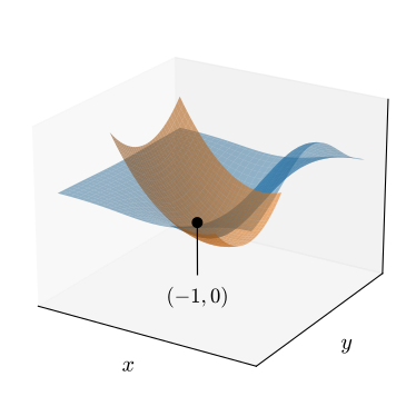
The figure asserts agreement; we can check it numerically, exactly as we checked the gradient above. Evaluating \(f\) and its quadratic \(q\) at a few points stepping away from the base point, the gap should stay tiny nearby and grow with distance.
def f(x, y):
    return x * math.exp(-x**2 - y**2)

def quad(x, y):  # 2nd-order Taylor of f at the base point (-1, 0)
    return math.exp(-1) * (-1 - (x + 1) + (x + 1)**2 + y**2)

for d in [0.0, 0.05, 0.1, 0.3]:  # step d in each coordinate from (-1, 0)
    x, y = -1 + d, d
    print(f'step {d:.2f}: f = {f(x, y):.6f}, '
          f'quadratic = {quad(x, y):.6f}, gap = {abs(f(x, y) - quad(x, y)):.6f}')
step 0.00: f = -0.367879, quadratic = -0.367879, gap = 0.000000
step 0.05: f = -0.384315, quadratic = -0.384434, gap = 0.000119
step 0.10: f = -0.396388, quadratic = -0.397310, gap = 0.000921
step 0.30: f = -0.391929, quadratic = -0.412025, gap = 0.020096The gap vanishes at the base point and is third order in the step (doubling the step roughly multiplies it by eight), the third-order behavior promised above. Iterating this idea, repeatedly fitting the local quadratic and jumping to its minimum, is Newton’s method, which Section 25.1.4.4 introduced in one variable; Section 9.2 develops it as a practical optimizer.
25.2.4.2 The Second-Derivative Test
At a critical point of a twice continuously differentiable function, a definite or indefinite Hessian classifies local behavior; a semidefinite Hessian does not. At a critical point \(\mathbf{x}_0\) the gradient term in Equation 25.2.8 vanishes, so the local picture is purely quadratic,
\[ f(\mathbf{x}) - f(\mathbf{x}_0) \approx \frac{1}{2}(\mathbf{x}-\mathbf{x}_0)^\top \mathbf{H} f (\mathbf{x}_0)(\mathbf{x}-\mathbf{x}_0). \]
Stepping a unit direction \(\mathbf{v}\) away from \(\mathbf{x}_0\) makes the right-hand side \(\tfrac12\mathbf{v}^\top\mathbf{H}\mathbf{v}\): the scalar \(\mathbf{v}^\top\mathbf{H}\mathbf{v}\) is the second directional derivative of \(f\) along \(\mathbf{v}\), the second-order analogue of \(\mathbf{v}\cdot\nabla f\). At a critical point, where the slope term is gone, it is the curvature of \(f\) along \(\mathbf{v}\). Whether \(f\) goes up or down as we leave \(\mathbf{x}_0\) is governed entirely by the sign of this quadratic form, that is, by the definiteness of the symmetric matrix \(\mathbf{H}\). The classification is read straight off the eigenvalues of \(\mathbf{H}\) via the PSD/PD criterion of Section 24.2.3.2:
- \(\mathbf{H} \succ 0\) (all eigenvalues positive): \(f\) curves upward in every direction. Quantitatively, the quadratic term is at least \(\tfrac12\lambda_{\min}\|\mathbf{v}\|^2\) for a step \(\mathbf{v}\), where \(\lambda_{\min} > 0\) is the smallest eigenvalue, and this dominates the approximation’s \(o(\|\mathbf{v}\|^2)\) error for all small \(\mathbf{v}\), so \(\mathbf{x}_0\) is a strict local minimum.
- \(\mathbf{H} \prec 0\) (all eigenvalues negative): \(f\) curves downward everywhere, so \(\mathbf{x}_0\) is a local maximum.
- \(\mathbf{H}\) indefinite (eigenvalues of both signs): \(f\) rises along some directions and falls along others: a saddle.
- \(\mathbf{H} \succeq 0\) with a zero eigenvalue (semidefinite): the quadratic is flat along that eigenvector and second order is inconclusive; the behavior is decided by higher-order terms.
These local shapes (the bowl, the saddle, and the flat-bottomed trough of the semidefinite case) are exactly the quadratic-form surfaces drawn in Figure 24.2.4.
This is the multivariable generalization of the single-variable test \(f'' > 0\): there, curvature is a single number; here it is a matrix, and “positive curvature” becomes “positive definite.” Identity Equation 24.2.13 makes the upward-curving picture precise, writing the quadratic form as a weighted sum of squares over the eigenvector directions with the eigenvalues as weights.
The test is one we can run. The surface of Figure 25.2.6, \(f(x, y) = xe^{-x^2-y^2}\), has exactly two critical points: setting \(\frac{\partial f}{\partial x} = (1 - 2x^2)\,e^{-x^2-y^2}\) and \(\frac{\partial f}{\partial y} = -2xy\,e^{-x^2-y^2}\) to zero forces \(y = 0\) and \(x = \pm 1/\sqrt{2}\). The next cell assembles each Hessian from symmetric second differences (the same quantity \(\Delta_h\) that proved the Clairaut–Schwarz theorem), reads off the eigenvalues of a \(2 \times 2\) symmetric matrix in closed form, and prints the classification.
# Classify the critical points (+-1/sqrt(2), 0) of f(x, y) = x e^(-x^2-y^2)
def hessian(f, x, y, h=1e-4):  # symmetric second differences
    fxx = (f(x + h, y) - 2 * f(x, y) + f(x - h, y)) / h**2
    fyy = (f(x, y + h) - 2 * f(x, y) + f(x, y - h)) / h**2
    fxy = (f(x + h, y + h) - f(x + h, y - h)
           - f(x - h, y + h) + f(x - h, y - h)) / (4 * h**2)
    return fxx, fxy, fyy

for x0 in [-1 / math.sqrt(2), 1 / math.sqrt(2)]:
    fxx, fxy, fyy = hessian(f, x0, 0.0)
    mid, r = (fxx + fyy) / 2, math.sqrt(((fxx - fyy) / 2)**2 + fxy**2)
    lo, hi = mid - r, mid + r  # eigenvalues of [[fxx, fxy], [fxy, fyy]]
    kind = 'minimum' if lo > 0 else 'maximum' if hi < 0 else 'saddle'
    print(f'at ({x0:+.4f}, 0): eigenvalues {lo:+.3f}, {hi:+.3f} -> {kind}')
at (-0.7071, 0): eigenvalues +0.858, +1.716 -> minimum
at (+0.7071, 0): eigenvalues -1.716, -0.858 -> maximumAt \((-1/\sqrt{2}, 0)\) both eigenvalues are positive (\(\mathbf{H} \succ 0\), a strict local minimum) and at \((+1/\sqrt{2}, 0)\) both are negative, a local maximum; a saddle would show one eigenvalue of each sign, as in Exercise 5. This five-line loop is the second-derivative test as a program: differentiate twice (here numerically; autograd Hessians appear in Section 25.3), extract eigenvalues, read the signs.
The eigenvalue picture also explains why, in high dimension, saddles are the rule rather than the exception: a minimum requires all \(n\) eigenvalues to be positive at once, and if the signs at a random critical point behaved like independent coin flips, that would happen with probability \(2^{-n}\). The coin-flip heuristic can be made precise: for random Gaussian landscapes the statistics of critical points can be computed exactly and minima are exponentially outnumbered by saddles (Bray and Dean 2007), and the critical points actually encountered while training deep networks are overwhelmingly saddles too (Dauphin et al. 2014), one reason gradient methods fare better in practice than the old fear of “getting stuck in a bad local minimum” suggests.
The gradient, Hessian, and multivariable chain rule extend the one-variable methods to scalar functions of several variables. Neural network layers also map vectors to vectors and use matrix parameters. Their derivative is a matrix of partial derivatives, the Jacobian, with gradients and Hessians as special cases. The Mean Value Theorem of Section 25.1.4.2 does not survive the passage to vector-valued maps; only an inequality remains, the mean value inequality (Rudin 1976). Section 25.3 develops the Jacobian machinery, the layout conventions, and how it all yields backpropagation as reverse-mode automatic differentiation.
25.2.5 Summary
- The gradient \(\nabla_{\mathbf{w}} L\) is the derivative in many dimensions: it gives the first-order change \(L(\mathbf{w}+\boldsymbol{\epsilon}) \approx L(\mathbf{w}) + \boldsymbol{\epsilon}\cdot\nabla_{\mathbf{w}} L\), and its dot product with a unit direction is the rate of change along that direction.
- By Cauchy–Schwarz, \(+\nabla L\) is the direction of steepest ascent and \(-\nabla L\) of steepest descent, and the gradient is everywhere orthogonal to the level sets of \(L\): the geometry behind gradient descent.
- The multivariate chain rule sums, over every path from an input to the output, the product of edge derivatives. Organizing it from the output backward reuses every intermediate, giving backpropagation: a forward pass followed by a backward pass that yields the gradient with respect to all parameters at once.
- The symmetric Hessian supplies the second-order Taylor approximation; at a critical point its definiteness, read from its eigenvalues, distinguishes a minimum, a maximum, and a saddle.
25.2.6 Exercises
- Let \(L(x, y) = \log(e^x + e^y)\). Compute the gradient, and verify that the sum of its components is always \(1\). What does that say about the directions in which \(L\) grows fastest?
- For \(f(x, y) = x^2 + 2y^2\), compute \(\nabla f\) and verify at a sample point on the ellipse \(f = c\) that the gradient is orthogonal to the level curve.
- Prove directly from Equation 25.2.2 that at a local minimum the gradient must vanish.
- Let \(f(x, y) = x^3 - 3x + y^2\). Show that the critical points are \((\pm 1, 0)\). By examining \(f\) along the lines \(y = 0\) and \(x = \pm 1\), determine whether each is a minimum, a maximum, or a saddle, and confirm by computing the Hessian there.
- Classify the critical point of \(f(x, y) = x^2 - y^2\) by inspecting the eigenvalues of its (constant) Hessian. Why is this point a saddle?
- Give a two-variable \(f\) whose Hessian at a critical point is positive semidefinite (one zero eigenvalue) yet the point is not a local minimum. Why does the second-derivative test go silent here?
- Suppose we minimize \(f(\mathbf{x}) = g(\mathbf{x}) + h(\mathbf{x})\). Interpret the condition \(\nabla f = \mathbf{0}\) geometrically in terms of \(\nabla g\) and \(\nabla h\).
- Use the Lagrange condition Equation 25.2.4 to maximize \(f(x, y) = xy\) subject to \(g(x, y) = x + y = 1\). First check that \(\nabla g \neq \mathbf{0}\) everywhere, so the condition applies; then solve \(\nabla f = \lambda \nabla g\) together with the constraint, and confirm your answer by eliminating \(y = 1 - x\) and maximizing in one variable. Finally, replace the constraint by \(x + y = 1 + \delta\) and show that the maximum value changes by \(\lambda\delta\) to first order: the multiplier prices the constraint.